Research on Asymmetric Fault Location of Wind Farm Collection System Based on Compressed Sensing

Nomenclature

1  Introduction

In the 2020 ‘Wind Energy Beijing Declaration’, it is proposed to comprehensively consider the realistic feasibility of resource potential, technological progress trend, and grid-connected consumption conditions. In order to achieve the goal of connecting with the goal of carbon neutrality, in the ‘14th Five-Year Plan’, it is necessary to set the development space for wind power that is compatible with the national strategy of carbon neutrality: to ensure that the average annual increase in installed capacity is more than 50 million kilowatts. After 2025, the average annual increase in installed capacity of wind power in China should not be less than 60 million kilowatts, reaching at least 800 million kilowatts by 2030 and at least 3 billion kilowatts by 2060 [1]. The offshore wind farm collection system is composed of a large number of wind turbines. Most of the transmission lines in the collection system are buried deep in the seabed, which makes it difficult to locate the asymmetric fault and the fault recovery time is long. Therefore, when an asymmetric fault occurs in the collection system, its rapid and accurate positioning will help improve the utilization rate of wind power.

At present, the research methods for wind farm fault location mainly include the impedance method [2–5], the traveling wave method [6–8] and the deep learning method [9–14]. Reference [2] proposed a single-phase grounding fault location method based on successive search of fault sections, and introduced a logarithmic arc model describing the arc grounding of fault points to achieve high-ranging accuracy. In reference [3], the author constructed the impedance matching ranging algorithm from the first section to the section where the fault point is located by constructing a single interval ranging model and an equivalent injection current model of the fan branch. In reference [4], the author constructed a transmission equation containing the location of the fault point through the traveling wave characteristics. The overdetermined equations formed by the multi-point transmission equation are solved by the parameter estimation theory to obtain the fault location. Reference [5] proposed a combined ranging method for wind farm collector lines using a combination of matrix method and impedance method. In reference [6], the traditional traveling wave method is optimized to improve the accuracy of traveling wave detection, and the traveling wave velocity is optimized and corrected to realize the accurate location of the fault distance of the wind farm collector line and the transmission line. Reference [7] proposed a fault location method based on decision coefficient and extreme-point symmetric mode decomposition-Teager energy operator (ESMD-TEO). Reference [8] deduced a calculation method of modified traveling wave velocity based on the principle of single-ended traveling wave and combined with double-ended asynchronous information. Reference [9] collected the fault data of the collecting line of the wind farm and trained the deep learning neural network to establish a prediction model for single terminal fault location. Reference [10] proposed a new spatio-temporal multiscale neural network (STMNN). The proposed STMNN model contains two parallel feature extraction modules: first, a multiscale deep echo state network module to extract temporal multiscale features; second, a multiscale residual network module to extract spatial multiscale features. Reference [11] proposed a new multi-level denoising autoencoder (MLD-AE) method, which enhances the representation learning ability by designing different multi-level noise addition schemes based on the multivariate data-driven fault detection (MDFD) framework. Reference [12] proposed a hybrid fault detection system based on single input generalized regression neural network ensemble (GRNN-ESI) algorithm, principal component analysis (PCA) and wavelet probability density function (PDF). Reference [13] proposed a monitoring method based on conditional convolution autoencoder, which has duality and can be used to identify the damage of wind turbine blades. Reference [14] proposed an anomaly detection method for wind turbine gearbox based on adaptive threshold and double support vector machine (TWSVM). Furthermore, some new but important work in fault diagnosis is worth investigating. Reference [15] proposed a class-imbalanced privacy-preserving federated learning framework for distributed wind turbine fault diagnosis that incorporates a separate gradient-based self-monitoring scheme to identify global imbalance information for class-imbalanced fault diagnosis. A novel framework for multi-domain vibration feature extraction, feature selection, and cost-sensitive learning methods was developed in reference [16]. Extensive experiments show that multi-domain feature extraction and feature selection can improve diagnostic accuracy significantly.

In summary, the impedance method uses the voltage and current data obtained at the measuring point after the fault occurs, and the total impedance of the fault circuit is calculated by the voltage equation constructed by the circuit, and then the fault distance is obtained [17]. However, the initial current of the collection system is not only affected by the fault point shape, but also by the output of the wind turbine on different branches. Therefore, it is difficult to list an accurate fault loop voltage equation only based on the measured value of the collector line. For the traditional traveling wave method, due to the complex lines in the wind farm and the short transmission lines between the wind turbines, the refraction and reflection of the traveling wave after the fault are complex and changeable. Therefore, it is difficult to use the traveling wave method for fault location, and the traveling wave device is expensive. The deep learning method has a long training time, and the algorithm requires a large amount of fault data for operation and learning. However, the wind farm has high real-time requirements and it is difficult to provide so much measured data.

Compressed sensing theory has been increasingly used in the field of power system fault location in recent years. Reference [18] achieved accurate fault location based on sparse measurement by combining the node high-frequency voltage equation with the compressed sensing theory based on the Bayesian algorithm. Reference [19] proposed a single-ended fault location method based on atomic decomposition and traveling wave natural frequency. The Dice coefficient atom matching criterion and Fourier transform were introduced in reference [20] to improve the regularized orthogonal matching pursuit (ROMP) algorithm in the over-complete dictionary design to improve accuracy and achieve accurate fault location of HVDC lines.

Based on the above analysis, this paper analyzes the fault current sparsity characteristics in the wind farm collection system when asymmetric faults occur. Taking advantage of the fact that the negative sequence current generated by the wind turbine generator is almost zero when an asymmetric fault occurs in the system, the mathematical model of compression sensing is built through the node voltage equation. In the process of fault location, the phase-locked loop trigonometric function method is used to extract the fault negative sequence voltage, and the node impedance matrix is combined with the fault location coefficient to construct a new over-complete dictionary λ-NIM dictionary (λ-Node Impedance Matrix dictionary, λ-NIM). The algorithm is then improved by employing generalized Jaccard coefficients, yielding a generalized Jaccard Compressive Sampling matching pursuit (J-CoSaMP) algorithm. The algorithm is then used to locate the fault zone. Finally, using the ranging equation, the fault location is precisely determined based on the fault interval. The proposed method is anti-noisy and is less affected by fault location and transition resistance, allowing it to locate the fault accurately and quickly.

2  Fault Current Characteristic Analysis and Equivalent Replacement of Wind Farm

2.1 Analysis of Fault Current Sparse Characteristics

To be connected to the power grid, the wind turbines in the wind farm must pass through their respective box transformers, collection systems, transmission lines, and main transformers. Collection lines and collection buses are part of the collection system. Fig. 1 depicts the topology of the wind farm collection system.

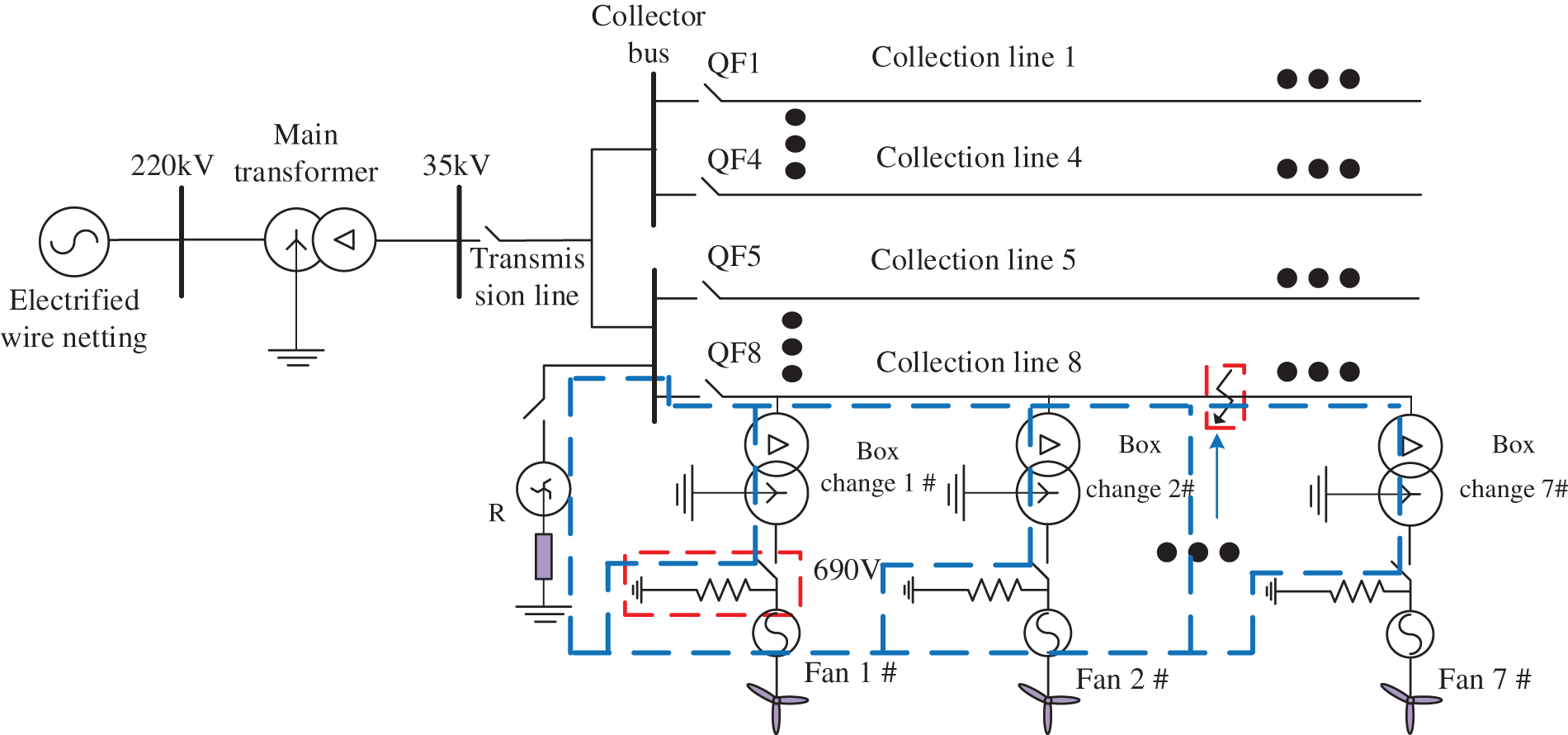
Figure 1: Topology of wind farm collection system

Because of the wind farm collection system’s asymmetric faults, namely single-phase ground fault, phase-to-phase fault, and two-phase ground fault, the negative sequence current emitted by the wind turbine is very small, almost negligible in comparison to the negative sequence current injected at the fault point. The negative sequence current flow path is shown in Fig. 2 when a single-phase ground fault, inter-phase fault, or two-phase ground fault occurs in the collection system.

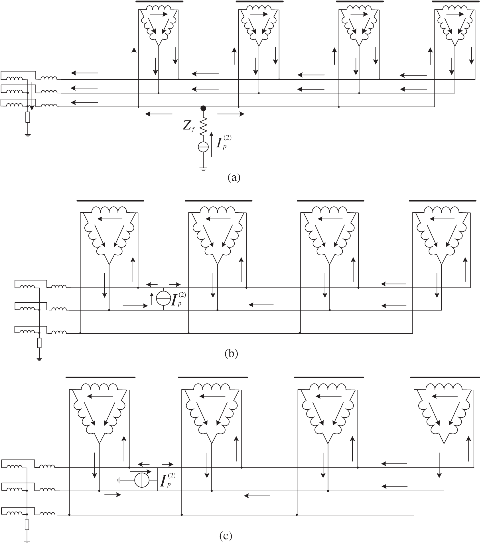
Figure 2: Negative sequence current flow path diagram. (a) Negative sequence current flow path in single-phase grounding fault, (b) Negative sequence current flow path in single-phase grounding fault, (c) Negative sequence current flow path in two-phase grounding fault

The short-circuit current negative sequence component I(2) in the wind farm collection system is only composed of the fault point negative sequence current, as shown in Fig. 2, and its expression is:

I(2)=IP(2)(1)

As a result, the fault negative sequence current is sparse, which meets the requirement of using compressed sensing theory. However, because underdetermined equations must be constructed in power system fault location, the compressed sensing theory can be introduced, and the negative sequence current just meets this condition. It flows into the earth from the three-phase load via the box-type transformer, resulting in the presence of the negative sequence current component in all transmission lines in the collection system. The node negative sequence voltage equations are written when the negative sequence voltage component and the node impedance matrix are combined. The underdetermined equations can be constructed by equivalently replacing the fault negative sequence current. Because single-phase ground faults account for the majority of asymmetric faults in wind farm collection systems, this paper chooses the single-phase ground fault experimental research object.

2.2 Equivalent Replacement of Fault Current

This paper selects the negative sequence current for equivalent substitution by analyzing the sparse characteristics of the acquisition system’s fault current. Using the wind farm collection system with N nodes as an example, the fault component negative sequence network’s node equivalent current substitution equation ΔU=Z×I is constructed, as shown in Eq. (2). I is the equivalent component of the fault negative sequence current, Z is the node impedance matrix, and ΔU is the fault negative sequence voltage component.

[ΔU1(2)⋮ΔUm(2)ΔUn(2)⋮ΔUN(2)]N×1=[Z11⋯Z1mZ1n⋯Z1N⋮⋱⋮⋮⋱⋮Zm1⋯ZmmZmn⋯ZmNZn1⋯ZnmZnn⋯ZnN⋮⋱⋮⋮⋱⋮ZN1⋯ZNmZNn⋯ZNN]N×1[I1(2)⋮Im(2)In(2)⋮IN(2)]N×1(2)

where ΔUi(2)=Ui(a)−Ui(2) is the negative sequence voltage component of node i, when the wind farm collection system does not fail, the negative sequence component and the zero sequence component in the system do not exist. As a result, the negative sequence component Ui(a) of node I prior to system failure has a value of 0, whereas the negative sequence component of node i following failure has a value of Ui(2).

A single-phase grounding fault develops between nodes m and n, as depicted in Fig. 3. Line impedance between nodes is Zmn, and the fault location coefficient, which measures the proportion of the line’s entire length (0, 1) that is traveled from node m to the fault point p, is λ.

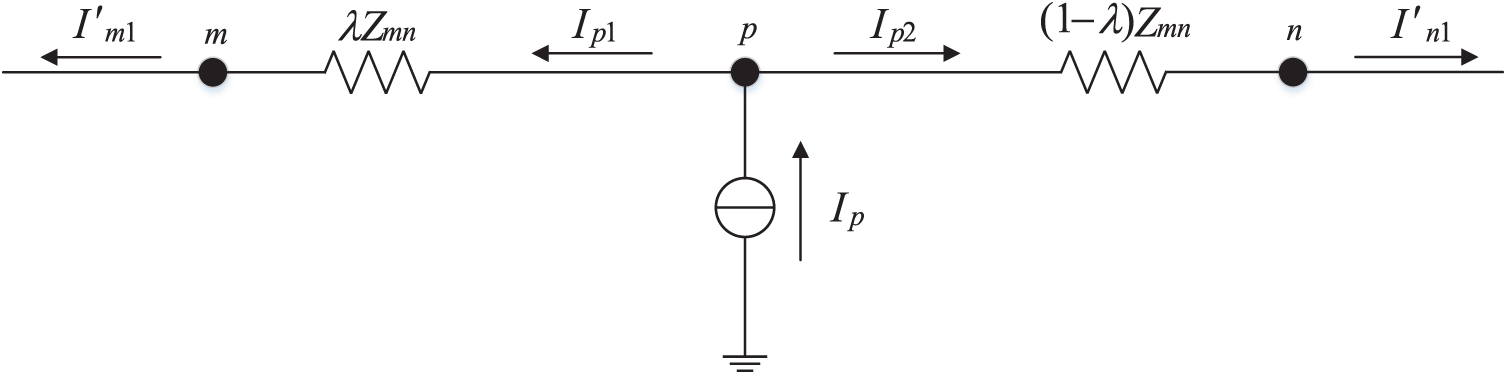
Figure 3: Schematic diagram of inter node fault

From Fig. 3:

{Umn=−λZmnIp1+(1−λ)ZmnIp2Ip=Ip1+Ip2(3)

where Umn is the potential difference between node m and node n; Ip is the fault negative sequence current source; Ip1 and Ip2 are negative sequence current flowing from fault point to node m and node n.

From Fig. 4:

{Umn=Zmn(Ipm−Ipm1′)Ipm=Ipm1′+Ipm1Ipn=Ipn1′+Ipn1(4)

where Ipm and Ipn are the virtual equivalent current sources of the fault negative sequence current source Ip replaced by node m and node n, respectively; Ipm1′ and Ipn1′ are the sum of all negative sequence currents outside nodes m and n after Ip replacement; Ipm1 is the negative sequence current flowing from node m to node n; Ipn1 is the negative sequence current from node n to node m.

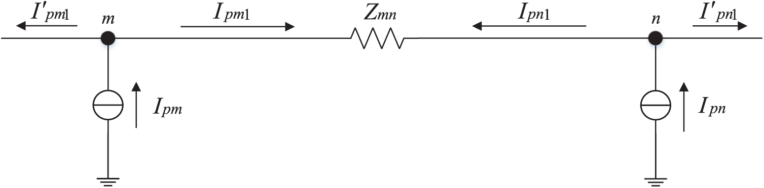
Figure 4: Schematic diagram of fault between nodes after equivalent

According to the KCL law, the nodes m and n, as well as the lines connecting them, can be considered as a whole, and the current of the outer line remains constant both before and after equivalence, that is:

{Ipm1′=Im1′Ipn1′=In1′(5)

where Im1′ and In1′ are the sum of all negative sequence currents outside nodes m and n before the fault negative sequence current source is replaced Ip.

The equivalent substitution relation of fault negative sequence current can be obtained by combining Eqs. (3)–(5):

{Ipn=λIpIpm=(1−λ)IpIpm+Ipn=Ip(6)

When a fault occurs, a single fault negative sequence current source in Fig. 2 can be equivalent to a virtual equivalent current source of two adjacent nodes, as shown by Eq. (6). As shown in Fig. 3, the node’s negative sequence voltage equation is:

[ΔU1(2)⋮ΔUm(2)ΔUn(2)⋮ΔUN(2)]N×1=[Z11⋯Z1mZ1n⋯Z1N⋮⋱⋮⋮⋱⋮Zm1⋯ZmmZmn⋯ZmNZn1⋯ZnmZnn⋯ZnN⋮⋱⋮⋮⋱⋮ZN1⋯ZNmZNn⋯ZNN]N×1[0⋮Im(2)In(2)⋮0]N×1(7)

Although the Eq. (7) is made up of N equations, in practice, only M (M < N) nodes are chosen to install the voltage measuring device in the entire collection system, and M equations are obtained as follows:

[ΔUi1(2)ΔUi2(2)⋮ΔUiM(2)]M×1=[Zi11Zi12⋯Zi1NZi21Zi22⋯Zi2N⋮⋮⋱⋮ZiM1ZiM2⋯ZiMN]M×N[0⋮Im(2)Im(2)⋮0]N×1(8)

where ΔUi1(2) denotes the negative sequence voltage component at node 1 following the failure of node i. Because Eq. (8) is an underdetermined system with a sparse fault quantity, the compressed sensing theory is used to accurately reconstruct the fault negative sequence current.

3  Fault Location Dictionary Design and Algorithm Improvement

3.1 Compressed Sensing Theory

By employing a lower sampling frequency algorithm, compressed sensing theory can recover the fault sparse vector. Its mathematical model is as follows:

y=Φx(9)

where y is the observation matrix; Φ is a sensing matrix; x is the fault sparse vector.

The reconstruction algorithm can be used to recover the fault sparse vector x from the measurement matrix y as follows:

min‖x‖0, s.t. y=Φx(10)

It is challenging to directly solve the l0 norm in Eq. (10) and it is an NP-hard problem [21]. According to published research [22], if the sensing matrix meets the Restricted Isometry Property (RIP) and δ∈(0,1):

(1−δ)‖x‖22≤‖Φx‖22≤(1+δ)‖x‖22(11)

The l0 norm and l1 norm can be transformed, that is:

min‖x‖1, s.t. y=Φx(12)

3.2 Fault Voltage Extraction and λ-NIM Dictionary Design

The extraction of negative sequence fault voltage amplitude and the choice of an over-complete dictionary will impair the accuracy of fault location when compressed sensing is introduced for fault location in accordance with Eq. (8). In order to generate the λ-NIM dictionary, this study enhances the fault voltage amplitude extraction scheme and incorporates the fault location coefficient in the node impedance matrix.

3.2.1 Fault Voltage Extraction Based on Phase-Locked Loop Trigonometric Function Method

The conventional voltage amplitude extraction method typically uses the instantaneous symmetrical component approach to extract the voltage component for the negative sequence fault. However, due to the peculiarities of the method, a non-model error will be produced at the voltage mutation point during the process of extracting the fault voltage, resulting in a spike occurrence, as illustrated in Fig. 5. The extracted negative sequence fault voltage amplitude deviation will cause reconstruction vector positioning inaccuracy, which is prone to erroneous fault points, and will also have an impact on the outcomes of the succeeding ranging when it is too great.

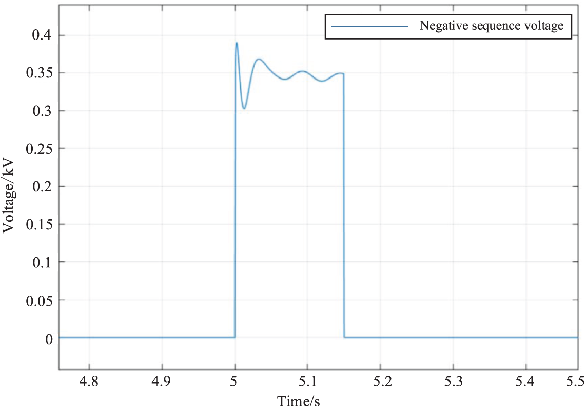
Figure 5: Extracting negative sequence voltage waveform by symmetrical component method

The conventional phase-locked loop trigonometric function method employs a low-pass filtering technique to reduce spike phenomena and improve fault location accuracy. When an asymmetric fault develops in the wind farm collection system, the collection line contains a large number of harmonic components. As a result, in this study [23], the active filter and phase-locked loop trigonometric function approaches are combined. The IGBT inverter module’s efficient filtering out of each harmonic improves the extraction accuracy of the fault voltage even more. Fig. 6 shows how well this strategy prevents the spike phenomenon. The overall flow chart is shown in Fig. 7.

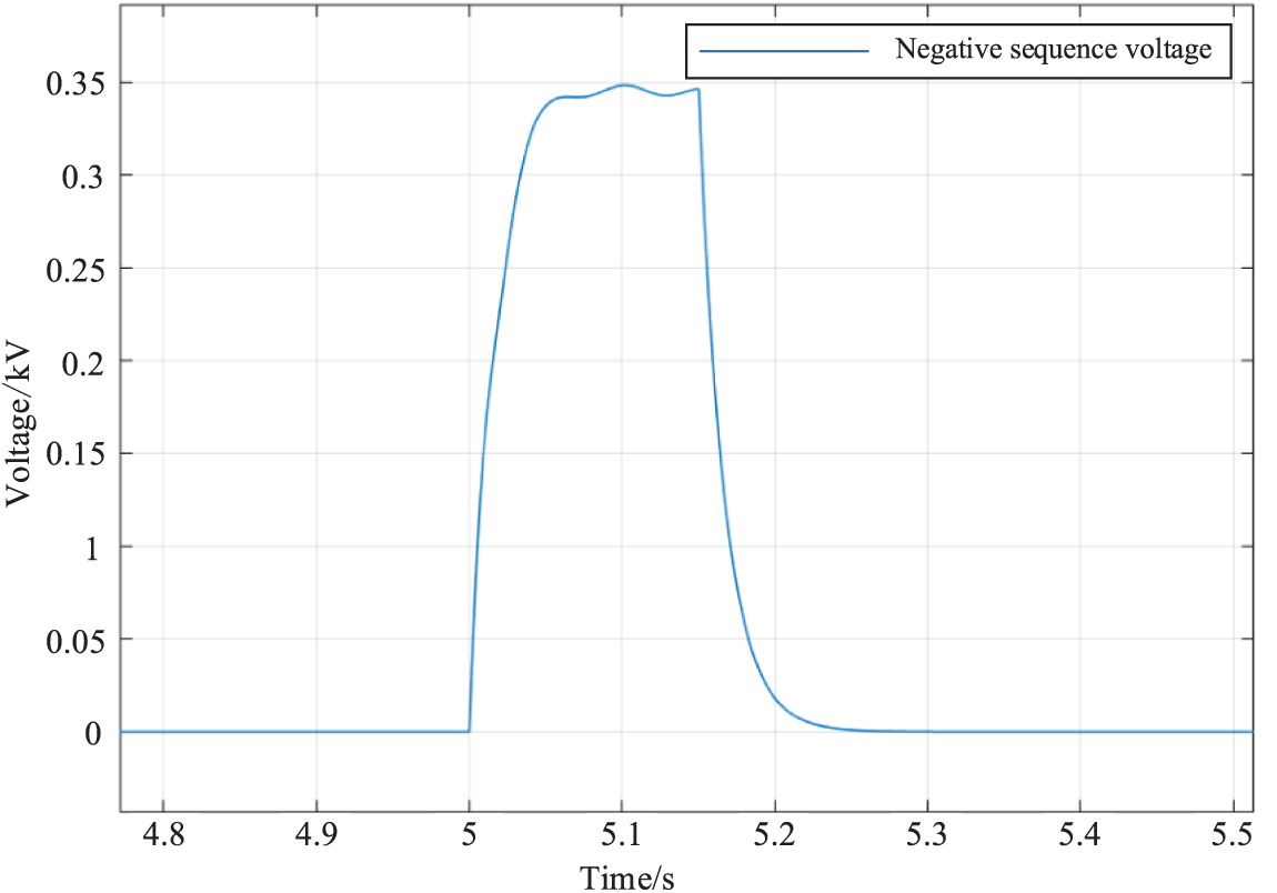
Figure 6: Extracting negative sequence voltage waveform by phase locked loop trigonometric function method

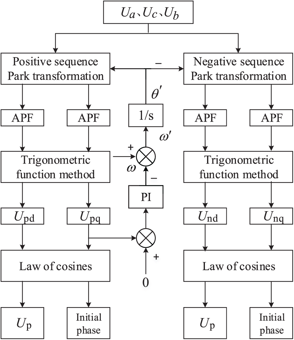
Figure 7: Phase locked loop trigonometric function method

3.2.2 Design Based on Fault Location Parameters λ-NIM Dictionary

The fault location coefficient is introduced in this paper to reduce the probability of false fault point and shorten the time of fault location. Eq. (7) is transformed, and the sparsity K of the fault negative sequence current is changed to 1, so that the fault location can be found with only one traversal in the subsequent algorithm reconstruction process. The value of fault current IP(2) is the square of the sum of the arithmetic square roots of the virtual equivalent current sources Im(2) and In(2). From Eq. (7):

{ΔUm(2)=Zmm⋅Im(2)+Zmn⋅In(2)ΔUn(2)=Znm⋅Im(2)+Znn⋅In(2)(13)

From Eqs. (6) and (7):

{ΔUm(2)=[(1−λ)⋅Zmm+λ⋅Zmn]⋅(Im(2)+In(2))ΔUn(2)=[(1−λ)⋅Znm+λ⋅Znn]⋅(Im(2)+In(2))(14)

Thus, by Eq. (14), Eq. (7) becomes:

[ΔU1(2)ΔU2(2)⋮ΔUN(2)]N×1=[(1−λ)Z11+λZ12(1−λ)Z12+λZ13⋯(1−λ)Z1,N−1+λZ1N(1−λ)Z21+λZ22(1−λ)Z22+λZ23⋯(1−λ)Z2,N−1+λZ2N⋮⋮⋱⋮(1−λ)ZN1+λZN2(1−λ)ZN2+λZN3⋯(1−λ)ZN,N−1+λZNN]N×1[0⋮IP(2)0]N×1(15)

However, because the fault location coefficient has a value range of (0, 1), when all of them are substituted into Eq. (15), the number of columns in the λ-NIM dictionary will reach hundreds of columns, resulting in a long convergence time for the compressed sensing algorithm. This paper estimates λ={λ1,λ2,⋯,λN}, where λ1 is the estimated value of the fault location coefficient between the first and second wind turbines; Ui(0) is the zero-sequence voltage at node i; R is the resistance of the grounding transformer; U0(0) is the zero-sequence voltage value at the collection bus; and Zij is the impedance value between nodes i and j.

λ1=U2(0)R−U0(0)R−U0(0)Z01U0(0)Z12(16)

λ2=U3(0)R−U0(0)R−U0(0)(Z01+Z12)U0(0)Z23(17)

λ3=U4(0)R−U0(0)R−U0(0)(Z01+Z12+Z23)U0(0)Z34(18)

{U2(0)Z12+Z01+R=U0(0)RU3(0)Z12+Z01+Z23+R=U0(0)RU4(0)Z12+Z01+Z23+Z34+R=U0(0)R(19)

The combined Eqs. (16)–(19) can be obtained:

{λ2=(λ1−1)⋅Z12Z23+1λ3=(λ2−1)⋅Z23Z34+1(20)

By the Eq. (20) can predict the value of λ = {λ1, λ2, ... , λN,}, then the Eq. (15) becomes:

[ΔU1(2)ΔU2(2)⋮ΔUN(2)]N×1=[(1−λ1)Z11+λ1Z12(1−λ2)Z12+λ2Z13⋯(1−λN−1)Z1,N−1+λN−1Z1N(1−λ1)Z21+λ1Z22(1−λ2)Z22+λ2Z23⋯(1−λN−1)Z2,N−1+λN−1Z2N⋮⋮⋱⋮(1−λ1)ZN1+λ1ZN2(1−λ2)ZN2+λ2ZN3⋯(1−λN−1)ZN,N−1+λN−1ZNN]N×1[0⋮IP(2)0]N×1(21)

3.3 J-CoSaMP Algorithm

To compute the residual modulus, the Jaccard-CoSaMP algorithm proposed in this paper employs the generalized Jaccard coefficient matching criterion [24] rather than the inner product criterion. The results are shown in Fig. 8.

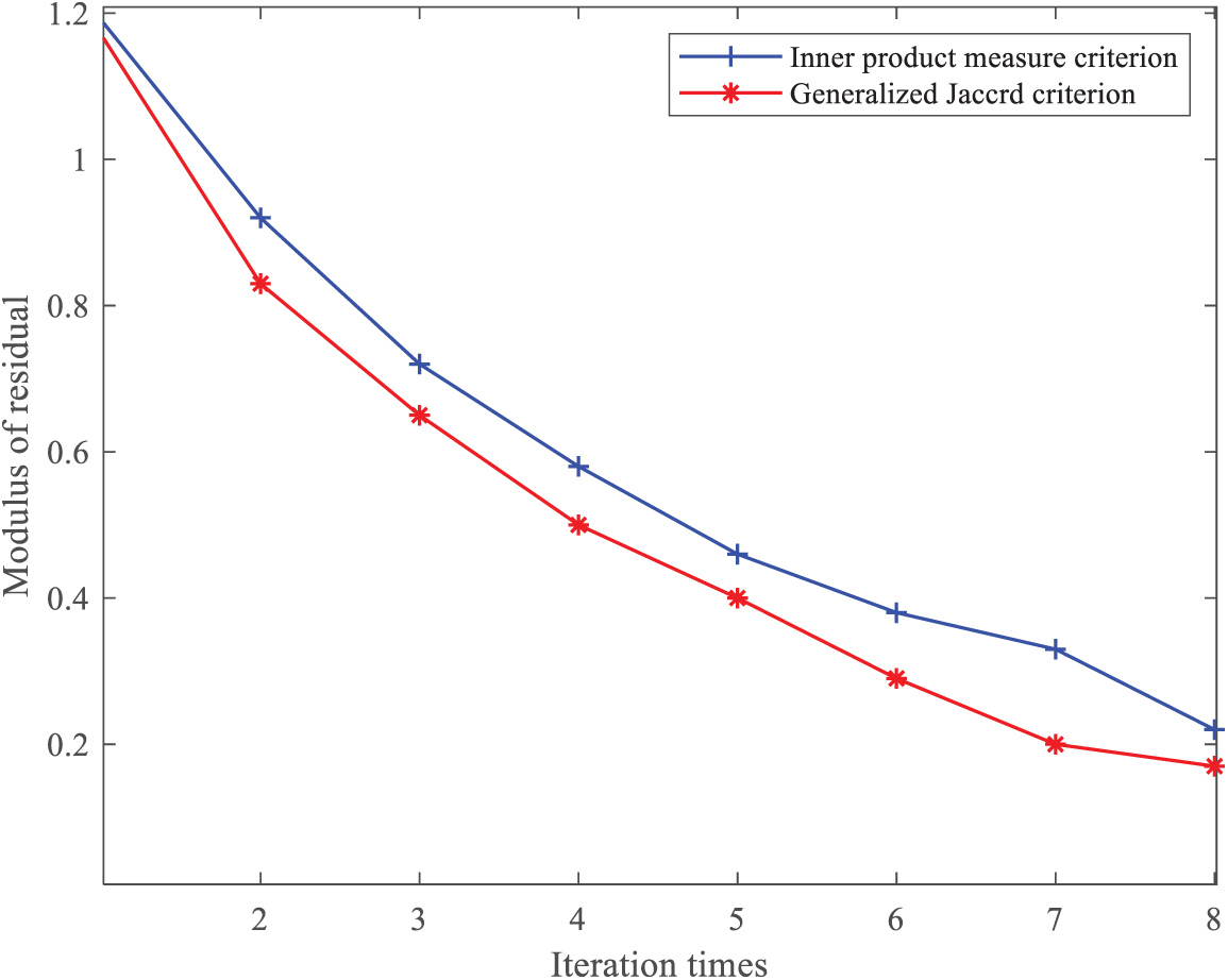
Figure 8: Comparison of residual calculation results

As a result, the difference between the selected atom and the residual signal is smaller when compared to the traditional algorithm. The data is then normalized to improve the rate of atomic convergence. The algorithm’s main steps are as follows:

Initialization: residual r0=y, index set Λ0=∅, support set A0=∅, t=1;

1. The correlation coefficient u is calculated by the generalized Jaccard coefficient matching criterion: u=|Jaccard(AT,rk−1)|; and normalized and arranged in descending order;

2. Select the maximum 2K values for the result of Step 1 to form the set aj and its corresponding subscripts to form J0; updating index set Λt=Λt−1∪J0 and support set At=At−1∪aj;

3. Using the least square method to find the least square solution of y=Atxt: x^t=argmin‖y−Atxt‖=(AtTAt)−1AtTy;

4. For the result of Step 3, K values with the largest absolute value are selected to form set x^tK, K columns in the corresponding support set are marked as AtK, the sequence number of the corresponding support set is marked as ΛtK, and index set Λt=ΛtK and residual rt=y−AtKx^tK are updated;

5. Get the reconstructed signal x^.

The specific steps of the algorithm are shown in Fig. 9.

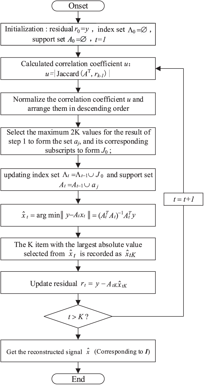
Figure 9: Flow chart of J-CoSaMP algorithm

4  Collection System Fault Location Equation and Steps

4.1 Fault Location Equation of Collecting System

When the negative sequence component I of the fault current is reconstructed using compressed sensing, it is fed into Eq. (21) to solve, and the negative sequence voltage amplitude of the adjacent nodes at both ends of the fault point is obtained. Following that, ranging is done in conjunction with impedance characteristics.

Reference [25] developed the ranging equation to accurately locate the fault by examining the negative sequence voltage components and impedance characteristics at both ends of the fault section. In the event of a system fault, the negative sequence network diagram is depicted in Fig. 10, and the distance between the fault and the negative sequence voltage is as follows:

ΔUm(2)ΔUn(2)=(1−λ)Zmn+ZnλZmn+Zm⋅ZmZn(22)

where Zm is the equivalent impedance of all lines before node m; Zn is the equivalent impedance of all lines after node n; Zmn is the mutual impedance between node m and node n.

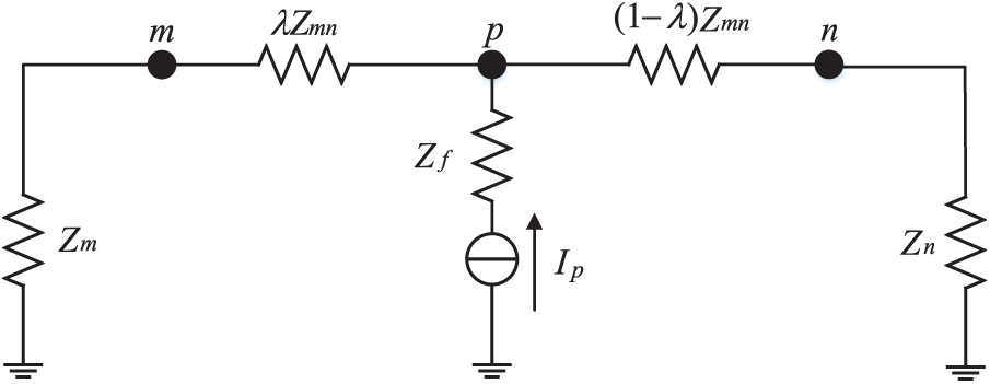
Figure 10: Fault zero sequence network diagram

The negative sequence voltage amplitude of two adjacent nodes is used in this paper to locate the fault using a Eq. (23):

|ΔUm(2)ΔUn(2)|=|(1−λ)Zmn+ZnλZmn+Zm|⋅|ZmZn|(23)

The number of unknowns in Eq. (23) for fault location is three, which are the fault location coefficient, Zm and Zn, respectively. As a result, the equivalent impedance values Zm and Zn must be calculated ahead of time. However, due to the complexity of the lines in the wind farm collection system, solving the equivalent impedance Zm and Zn directly is difficult. As a result, based on the wind farm collection system’s unique structural distribution characteristics, this paper proposes a method to solve the equivalent impedance.

During the design of the λ-NIM dictionary, the nodes m and n are viewed as a whole, and the injected fault negative sequence current is Ip. The flow path is shown in Fig. 11.

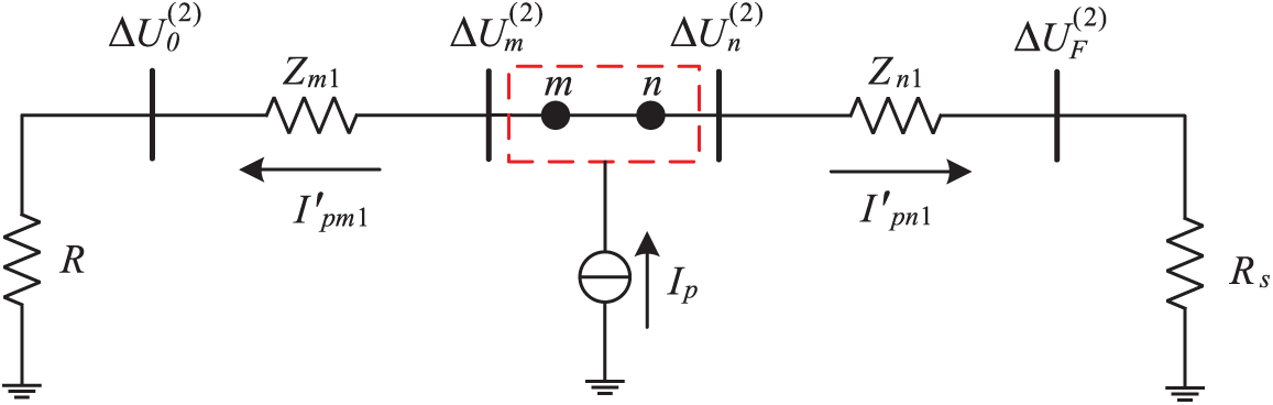
Figure 11: Fault current flow path diagram

As can be seen from Fig. 11:

{ΔUm(2)−ΔU0(2)Ipm1′=Zm1ΔU0(2)R=Ipm1′ΔUn(2)−ΔUF(2)Ipn1′=Zn1ΔUF(2)RS=Ipn1′(24)

where ΔU0(2) is the fault negative sequence voltage amplitude at the collection bus; ΔUF(2) is the fault negative sequence voltage amplitude at the last fan of the collection line; R is the resistance value of the grounding transformer; RS is the resistance value of the three-phase load; The equivalent impedance is Zm=Zm1+R, Zn=Zn1+RS.

The values ΔU0(2) and ΔUF(2) can be obtained after determining the fault interval by measuring the fault negative sequence voltage amplitude at the bus and the last fan of the collection line. As a result, using Eq. (24), the values Zm1 and Zn1 can be calculated, and the values of equivalent impedance Zm and Zn can be obtained. The only unknown variable in the Eq. (23) is the fault location coefficient λ. To create a quadratic equation, square both sides of Eq. (23):

(|ΔUm(2)ΔUn(2)|2|ZnZm|2−1)|Zm|2λ2+[|ΔUm(2)ΔUn(2)|2|ZnZm|2|Zmn||Zm|+|Zmn|2+|Zmn||Zn|]2λ+|ΔUm(2)ΔUn(2)|2|ZnZm|2|Zm|2−(|Zmn|+|Zn|2)=0(25)

When Eq. (25) is solved, two solutions can be obtained, with the solution satisfying 0<λ<1 being the fault distance. Because only one solution satisfies the condition in general, this method can meet the majority of the positioning requirements in practice.

4.2 Converging System Fault Location Steps

Combined with J-CoSaMP algorithm, the proposed fault location steps of wind farm collection system are as follows:

1. The branch addition method is used to calculate the node impedance matrix and introduce the fault location coefficient based on the topological structure and line parameters of the wind farm collection system. The distribution of the measuring points yields the corresponding λ-NIM dictionary.

2. For the purpose of obtaining the appropriate fault voltage negative sequence component ΔU(2), read the voltage data of the measuring point before and after the fault at a specific time.

3. The λ-NIM dictionary and ΔU(2) obtained in Steps 1 and 2 are used as parameters in the J-CoSaMP algorithm to compute the fault negative sequence current component I.

4. If you read ΔU(2) times in a row, go to Step 5, otherwise go back to Step 3.

5. To obtain the fault negative sequence voltage amplitude of the corresponding node in the fault interval, the reconstruction result I is substituted into Eq. (21).

6. The obtained negative sequence voltage amplitude and system impedance Zmn, Zm, and Zn are entered into Eq. (25) to solve, and the solution satisfying 0<λ<1 is chosen to locate the fault.

The flow chart is shown in Fig. 12.

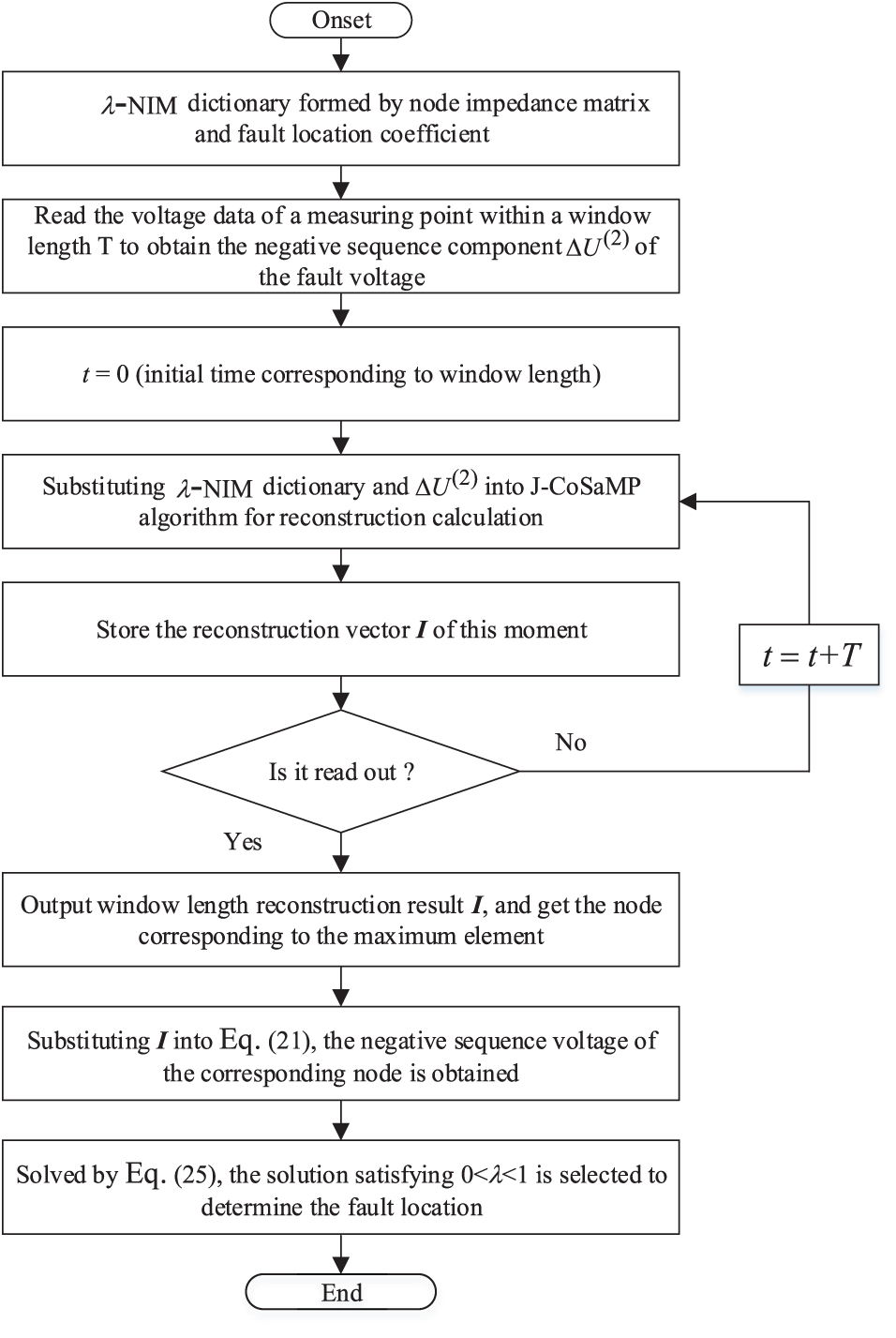
Figure 12: Fault location flow chart

In theory, the location of non-zero elements in the compressed sensing reconstruction result is the location of the fault node. However, it is difficult to ensure that the results of a reconstruction are accurate during the reconstruction process. As a result, in order to reduce the presence of false fault points, this paper reconstructs the same fault multiple times and selects the results with the most times to determine.

5  Experimental and Simulation Verification

5.1 Analysis of Short Circuit Experiment

The 35 kV collection system in a large wind farm with a rated capacity of 504 MW is used as the research object in this paper, and the Simulink simulation platform is built, as illustrated in Fig. 13. The system includes 56 wind turbines. The voltage of each wind turbine is raised to 35 kV by the box transformer. Following cable transmission to the collection bus, it is raised to 220 kV via the main transformer via the transmission line and sent to the power grid.

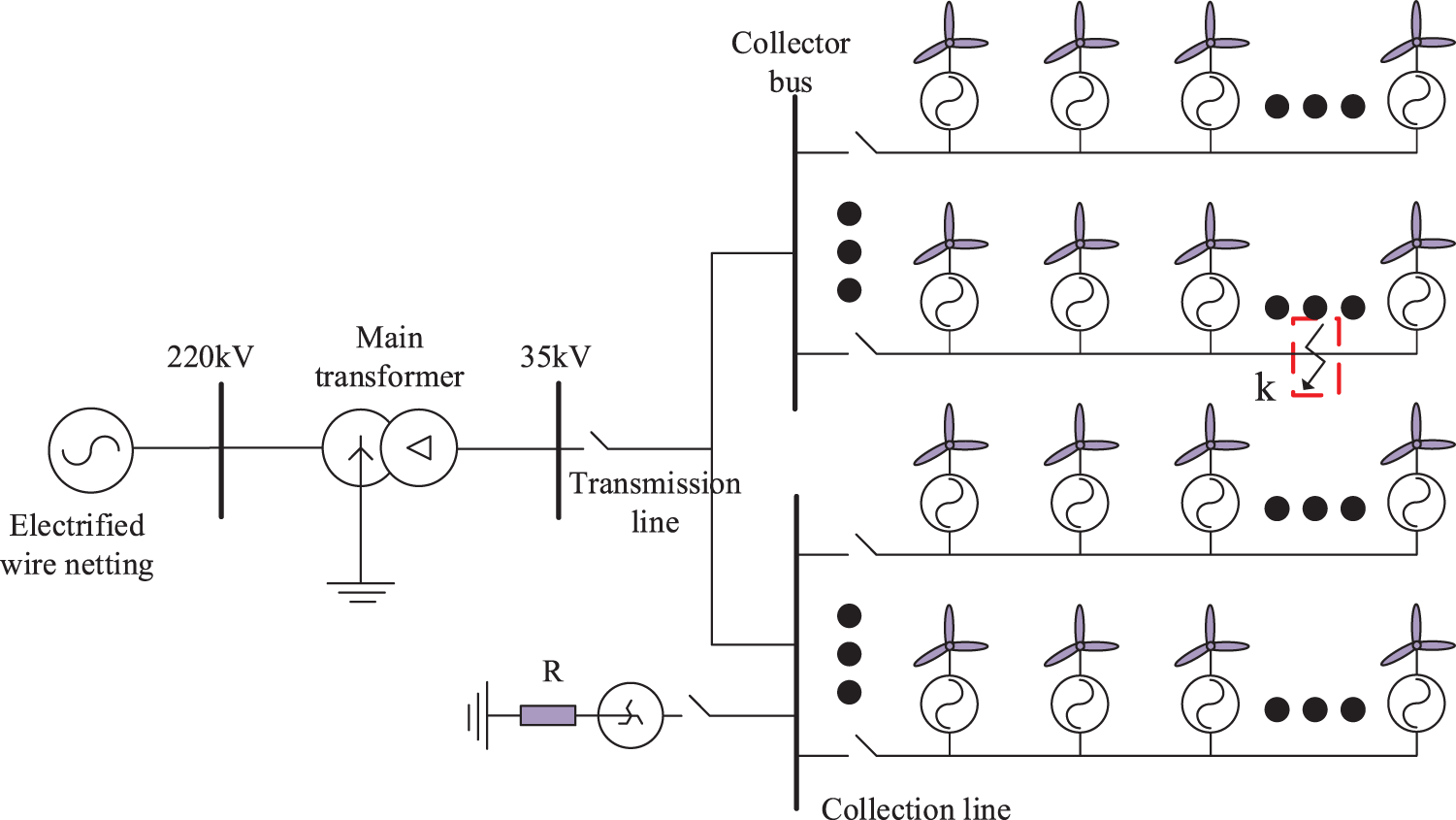
Figure 13: Topology of large wind farm collection system

The short-circuit experiment is performed on the collection system’s 35 kV collection line. As indicated by the k point in Fig. 13, the fault point is located on the collection line between the No. 12 and No. 13 fans. At 5 s, a phase-to-ground fault occurs, and at 5.15 s, the fault is removed. Fig. 14 depicts the three-phase current waveform on the collection line during the fault.

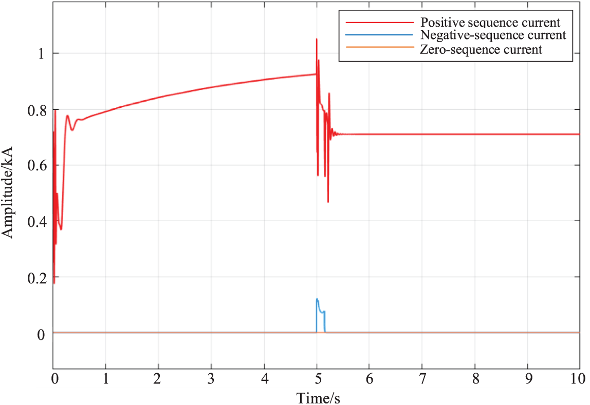
Figure 14: Three phase current waveform of fault line

The examination of the fault current sparse features of the wind farm collection system is validated by comparing Figs. 14 and 15. The fan’s negative sequence current output is 10−16 kA, or almost nil, when a single-phase grounding fault on the collecting line happens. In the wind farm collection system’s negative sequence network, the fault point is the only place where the fault negative sequence current is generated.

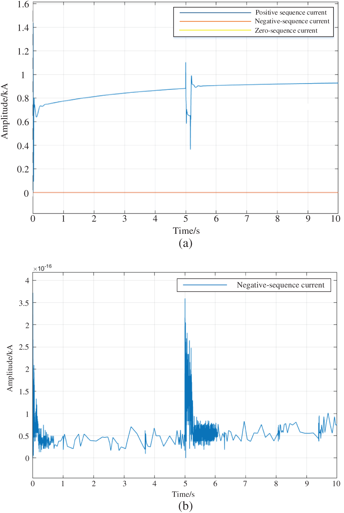
Figure 15: Current waveform of fan when fault occurs. (a) Three phase current waveform sent by the fan in case of fault, (b) Negative sequence current waveform sent by the fan in case of fault

5.2 Simulation Example of New Fault Location Algorithm

5.2.1 Fault Type and Location Impact Analysis

The distributed parameter model is primarily used in this paper, and a series of π-type equivalent circuits are used to simplify the modeling of a collection line in the wind farm collection system. Fig. 16 depicts the equivalent circuit. This circuit consists of series resistance R1, inductance L1, and grounding capacitance C1.

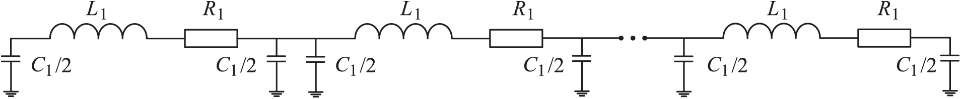
Figure 16: Simplified π unit based modeling

The parameter calculation of π type equivalent circuit is shown in Eq. (26):

{R1=lsR0L1=lsL0C1=lsC0(26)

where R0, L0, and C0 are the resistance, inductance, and capacitance per unit length of the cable line, respectively, and ls is the length of a single-type equivalent circuit.

When a single-phase ground fault occurs in the wind farm collection system, the negative sequence network structure is depicted in Fig. 17 (the line segments between the nodes represent line impedance and transformer impedance, etc.).

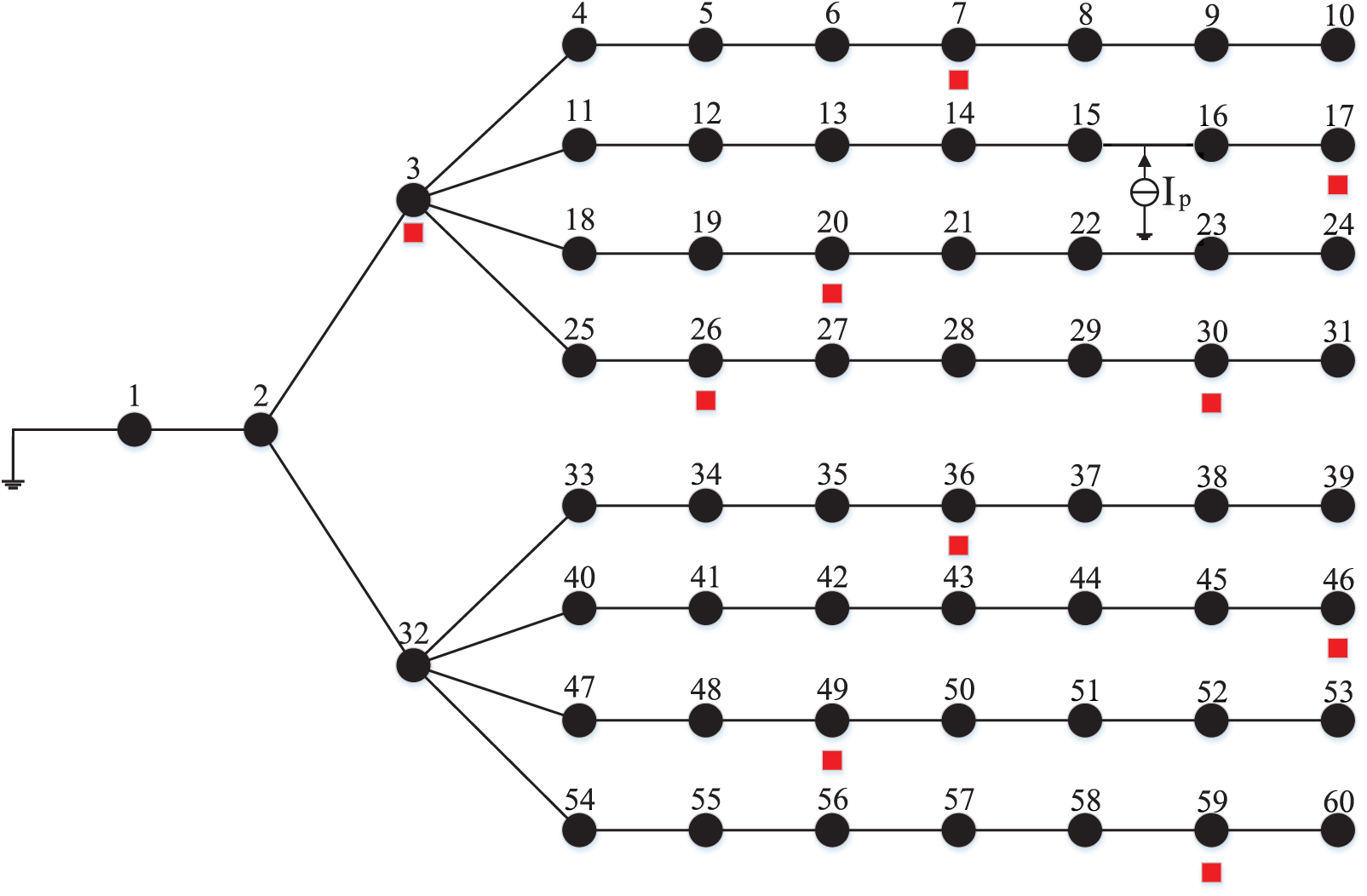
Figure 17: Negative sequence network diagram of collection system

(1) Failure mode

To make the following calculation easier, assume nodes 15 and 16 are 1 kM apart. If a single-phase ground fault occurs at a distance of 0.4 kM from node 15, the fault location coefficient is 0.4. At the same time, in order to ensure the accuracy of compressed sensing fault location, it is required that there is at least one measurement node in each collection line. Therefore, this paper selects 10 nodes of 3, 7, 17, 20, 26, 30, 36, 46, 49, and 59 in the collection system (60 nodes) as the measurement points to install the voltage measurement device, so that the 10 measurement nodes are evenly distributed in the wind farm collection system. The voltage data at the ten measuring points following the fault are recorded, and the amplitude of the fault negative sequence voltage is extracted using the phase-locked loop trigonometric function method, as illustrated in Table 1.

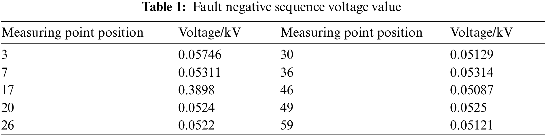
As shown in Fig. 18, the J-CoSaMP algorithm is used to reconstruct the fault negative sequence current component I. The node number is represented by the x-axis, and the amplitude of the fault negative sequence current is represented by the y-axis.

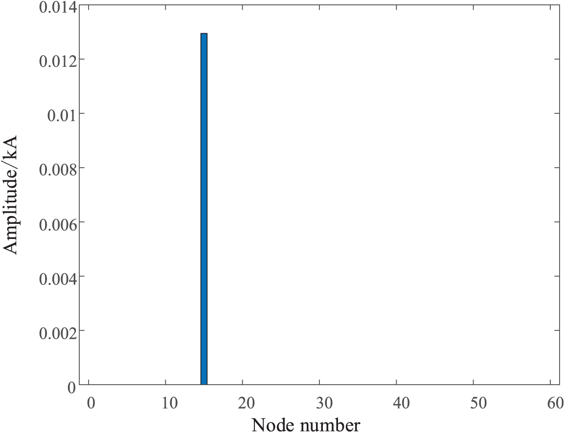
Figure 18: Vector I when nodes 15 and 16 fail A-0 Ω

The voltage amplitude is measured over a time range of 0.25–15.25 ms. 30 results can be obtained when the sampling frequency is set to 2 kHz. Fig. 19 depicts the fault negative sequence current component I at each instantaneous time. The x axis in the figure represents the node number, the y axis time, and the z axis the amplitude of the fault negative sequence current.

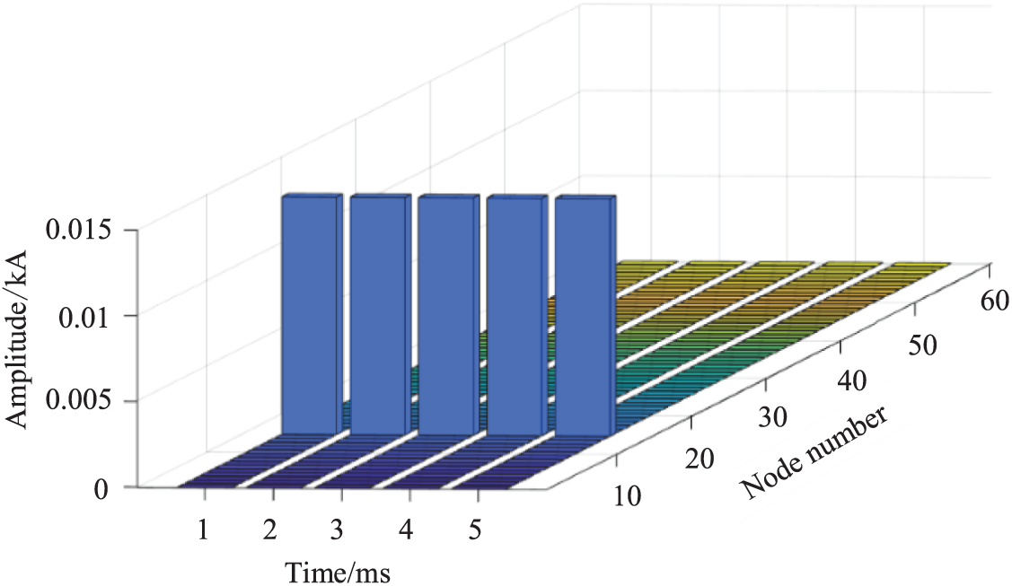
Figure 19: Reconstructed current vector I in each period

Section 4.1 states that after determining the fault occurrence interval, the obtained fault negative sequence current component I is substituted into Eq. (21) to obtain the voltage amplitudes of buses 15 and 16 of 0.3222 kV and 0.3875 kV, respectively. The negative sequence voltage amplitudes Zm and Zn are then entered into Eq. (25). The value of λ is 0.3991 according to the conditions for selecting roots in Section 3.1. By analogy, the fault location coefficient is 0.3987 until all 30 results are calculated and averaged. The fault distance is 0.3987 kM, the absolute error is 0.0013 kM, and the relative error is 0.325% because the distance between nodes 15 and 16 is 1 kM.

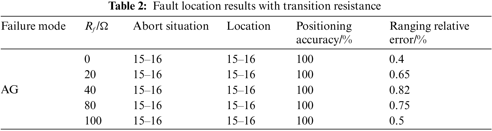
(2) Effect of transition resistance

This paper sets five different transition resistances Rf=10,20,40,80,100 for fault analysis when the fault occurs in order to study the influence of the transition resistance on the fault location of the wind farm collection system. Table 2 summarizes the simulation results. Because the element values in the node impedance matrix are constants, the transition resistance has no effect on them. Both the fault negative sequence current and the fault negative sequence voltage are variables. When the transition resistance varies, the value changes dramatically. As shown in Table 2, the transition resistance has no effect on the fault interval positioning results. Despite having an effect on the ranging results, the relative error is still less than 1%. As a result, the proposed method is less sensitive to transition resistance.

(3) Noise effect

This paper adds Gaussian white noise after reading the negative sequence voltage value to locate in order to investigate whether noise affects ranging error. Fig. 20 depicts the ranging’s relative error.

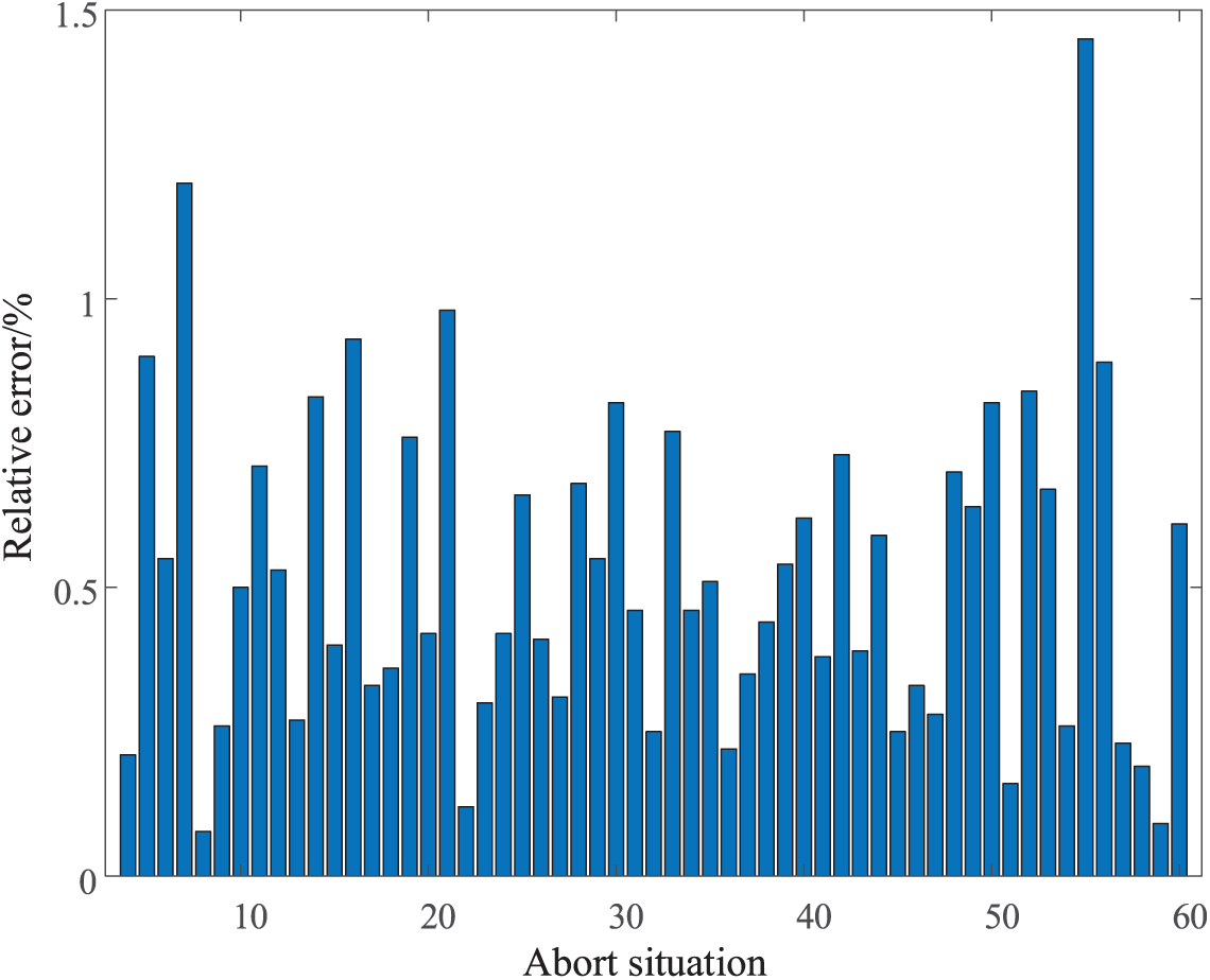
Figure 20: Relative error of each position during fault A-0 Ω

As shown in Fig. 20, the presence of noise increases the ranging relative error, but most of the errors are less than 1%, and in the actual situation of a wind farm collection system, the two fans are not far apart. As a result, a small amount of noise in the ranging process has little effect on the ranging results, and the proposed method’s anti-noise ability meets the practical application requirements.

5.2.2 Figure Labels and Captions

(1) Comparative analysis of fault voltage extraction schemes

Because the fault voltage reading value has a large influence on the fault interval positioning accuracy when using compressed sensing to reconstruct the fault negative sequence current. A single-phase ground fault is set between nodes 15 and 16 to see if the phase-locked loop trigonometric function method used in this paper can improve fault location accuracy. The fault voltage is extracted using the instantaneous symmetrical component method and the phase-locked loop trigonometric function method, and the fault interval is located using the J-CoSaMP algorithm. Table 3 displays the simulation results. In this paper, the reconstruction error is defined as the ratio of reconstruction failure times to reconstruction times.

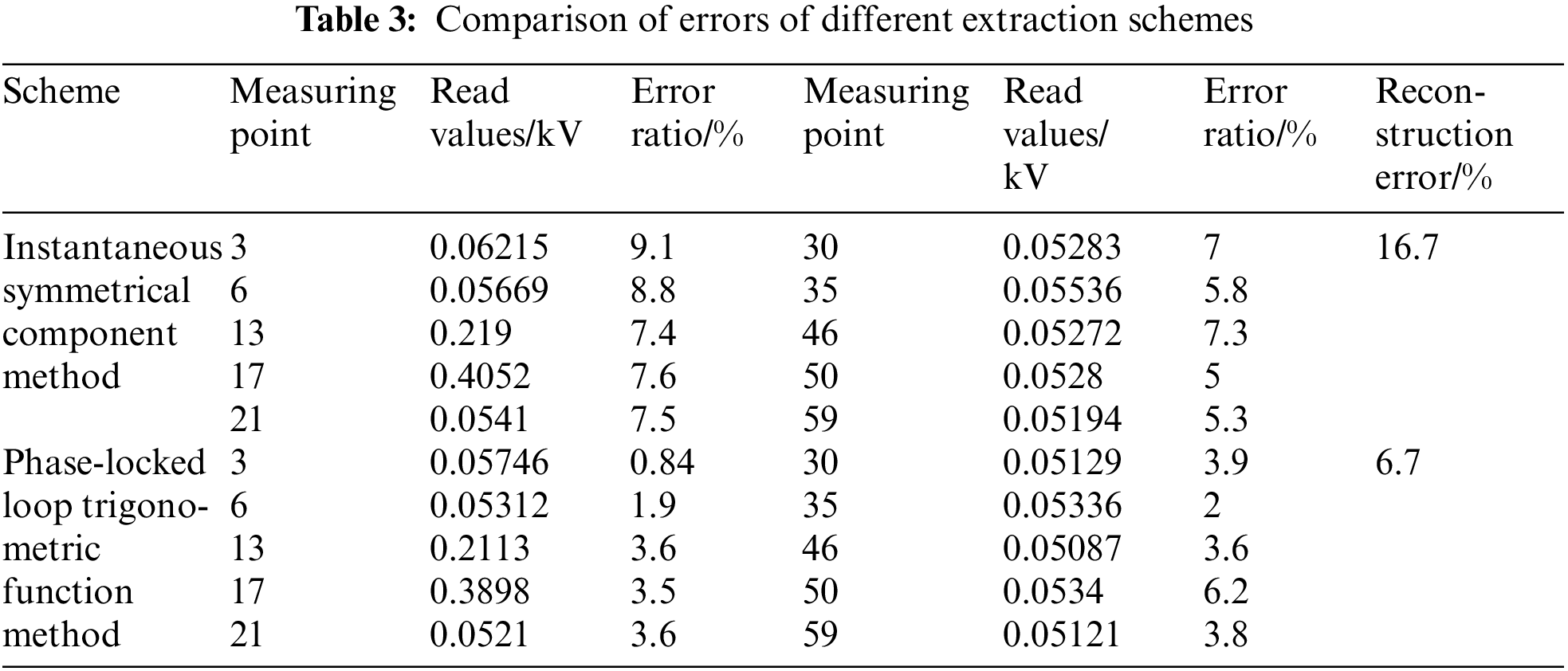
Table 3 shows that when using the instantaneous symmetrical component method to extract the fault voltage value, the error with the actual fault voltage value exceeds 5%, and the reconstruction error exceeds 16.7%. When using the phase-locked loop trigonometric function method to extract the fault voltage value, the error is typically less than 4%, and the reconstruction error is reduced to 6.7%. When calculating the fault voltage value, it can be seen that the phase-locked loop trigonometric function method is more accurate than the traditional instantaneous symmetrical component method. Meanwhile, during the fault location process, the phase-locked loop trigonometric function method can reduce reconstruction error and improve positioning accuracy.

(2) Comparative analysis of overcomplete dictionary selection

This paper uses a node impedance matrix and a λ-NIM dictionary to locate fault sections in order to investigate the effect of selecting an over-complete dictionary on fault section location accuracy. In the wind farm collection system, 23 nodes between nodes 4–26 are chosen to set up A-0 Ω grounding faults sequentially, and the reconstruction error is summarized in Fig. 21. Fig. 21 shows that when the node impedance matrix is used as the over-complete dictionary, the reconstruction errors of different fault points are mostly greater than 10%, with the maximum error being 33.3%. When using the λ-NIM dictionary for fault location, the reconstruction errors of various fault points are mostly reduced to less than 10%, demonstrating that using the λ-NIM dictionary for fault location can effectively improve fault location accuracy.

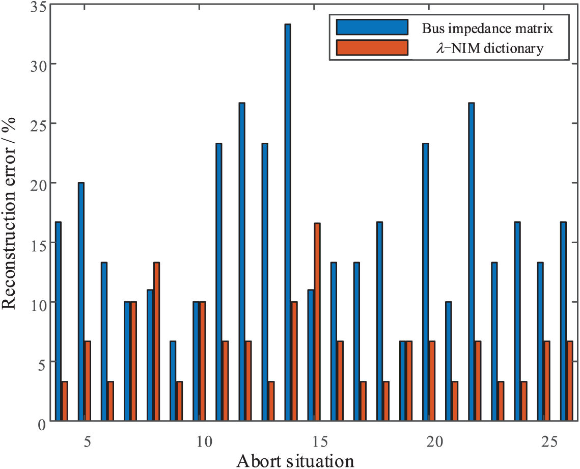
Figure 21: Reconstruction error of each position during fault A-0 Ω

(3) Comparative analysis of reconstruction algorithms

The compressed sensing reconstruction algorithm is enhanced in this paper. To investigate its improvement effect, the OMP algorithm, CoSaMP algorithm, and J-CoSaMP algorithm are used to locate the fault. Fig. 22 depicts the comparison results.

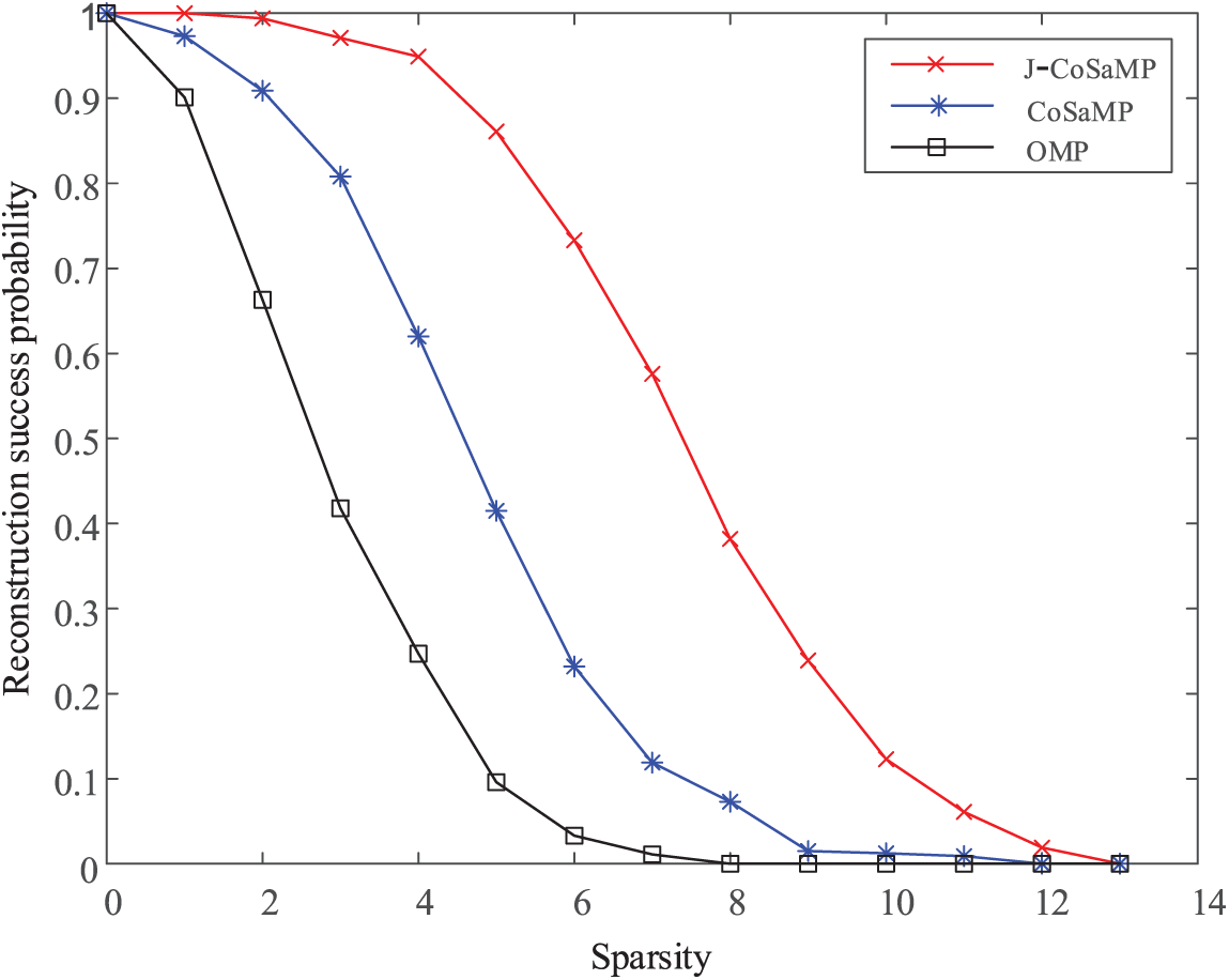
Figure 22: Algorithm reconstruction probability comparison chart

The figure shows that the sparsity K has a significant impact on the algorithm’s reconstruction success probability. The reconstruction success probabilities of the three algorithms used in this paper, namely the OMP algorithm, the CoSaMP algorithm, and the J-CoSaMP algorithm, are 97.3%, 90.1%, and 100%, respectively, when the sparsity is 1. When the sparsity is set to 2, the J-CoSaMP algorithm still has a 99.4% chance of successful reconstruction, whereas the other two algorithms have a 90.9% and a 66.3% chance, respectively. The comparison of the three algorithms demonstrates that the proposed algorithm can be applied to various sparsity conditions in the wind farm collection system and can effectively improve fault location accuracy.

(4) Ablation study

Ablation experiments are included to test the effectiveness of the phase-locked loop trigonometric function method, λ-NIM dictionary, and J-CoSaMP algorithm proposed in this paper. As an example:

a. Phase-locked loop trigonometric function method (PLTFM): The phase-locked loop trigonometric function method is replaced by the instantaneous symmetrical component method in this experiment, and the fault is located by combining the λ-NIM dictionary and the J-CoSaMP algorithm.

b. λ-NIM dictionary: The λ-NIM dictionary is replaced by a node impedance matrix in this experiment, and the fault is located by combining the phase-locked loop trigonometric function method and the J-CoSaMP algorithm.

c. J-CoSaMP algorithm: In this experiment, the J-CoSaMP algorithm is replaced by the CoSaMP algorithm, which is used in conjunction with the phase-locked loop trigonometric function method and the λ-NIM dictionary to locate the fault.

d. Integral experiment (IE): In this experiment, there is no variant, and the fault is found by combining the phase-locked loop trigonometric function method, the λ-NIM dictionary, and the J-CoSaMP algorithm.

To make a fair comparison, using the entire experiment as the reference group, a single-phase grounding fault with the same distance is set between nodes 15–16, 19–20, 34–35, 41–42, and 57–58, and 30 simulation experiments are performed. When performing fault location, all variants use the same parameter settings. Fig. 23 depicts the fault location results.

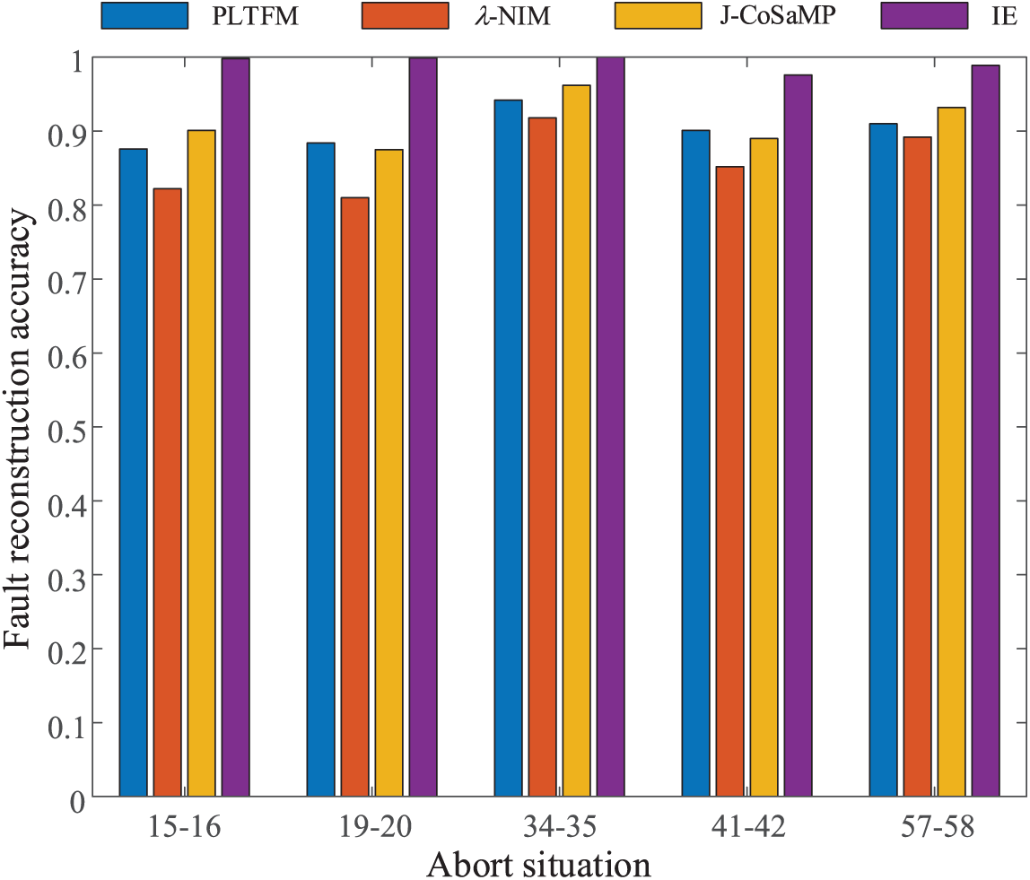
Figure 23: Comparison of performance on different variants

The λ-NIM dictionary has a significant influence on the accuracy of the method in this paper, as shown in Fig. 23 by comparing the three groups of experiments a, b, and c. That is, the λ-NIM dictionary makes the atoms in the observation matrix more matched by combining the fault location coefficient, which can significantly improve the fault location accuracy. Its improvement effect is clearly superior to the other two methods of improvement. Second, by comparing the two groups of a and c experiments, it can be seen that improving the extraction method and improving the algorithm have little difference in improving the proportion of fault location, but in general, the algorithm improvement is slightly larger than the extraction method improvement. As a result of the ablation experiment, the phase-locked loop trigonometric function method, λ-NIM dictionary, and J-CoSaMP algorithm proposed in this paper can effectively improve fault location accuracy, but the λ-NIM dictionary designed in this paper has a clear effect on fault location accuracy.

(5) Comparative analysis of fault location methods

The proposed method, impedance method [5], and traveling wave method [9] are used to locate a single-phase ground fault that is the same distance between nodes 15–16, 34–35, and 41–42. Table 4 displays the location results.

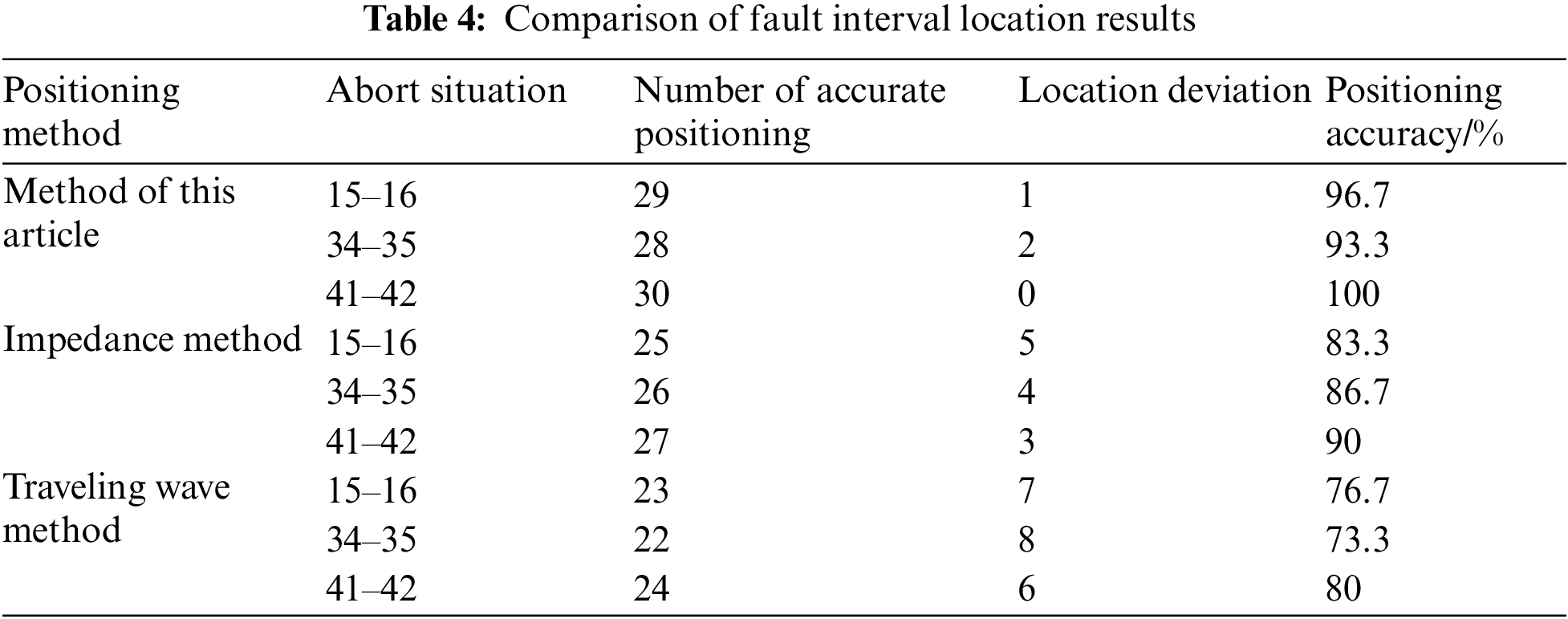
Table 4 shows that when the impedance method and the traveling wave method are used to locate the fault interval multiple times in the process of interval positioning of wind farm collection system faults, the positioning accuracy is generally below 90%, whereas the accuracy of the positioning method proposed in this paper is mostly above 90%. As a result, the proposed method outperforms the impedance method and the traveling wave method for interval positioning.

To investigate the overall performance of the fault location method proposed in this paper, single-phase ground faults of varying distances are placed between nodes 15–16, and the three methods listed in Table 4 are used to accurately locate faults. Table 5 shows the location results, and Fig. 24 shows the relative error of location.

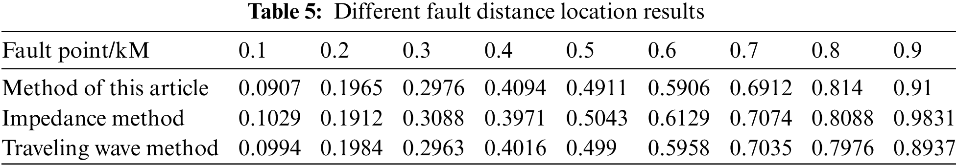
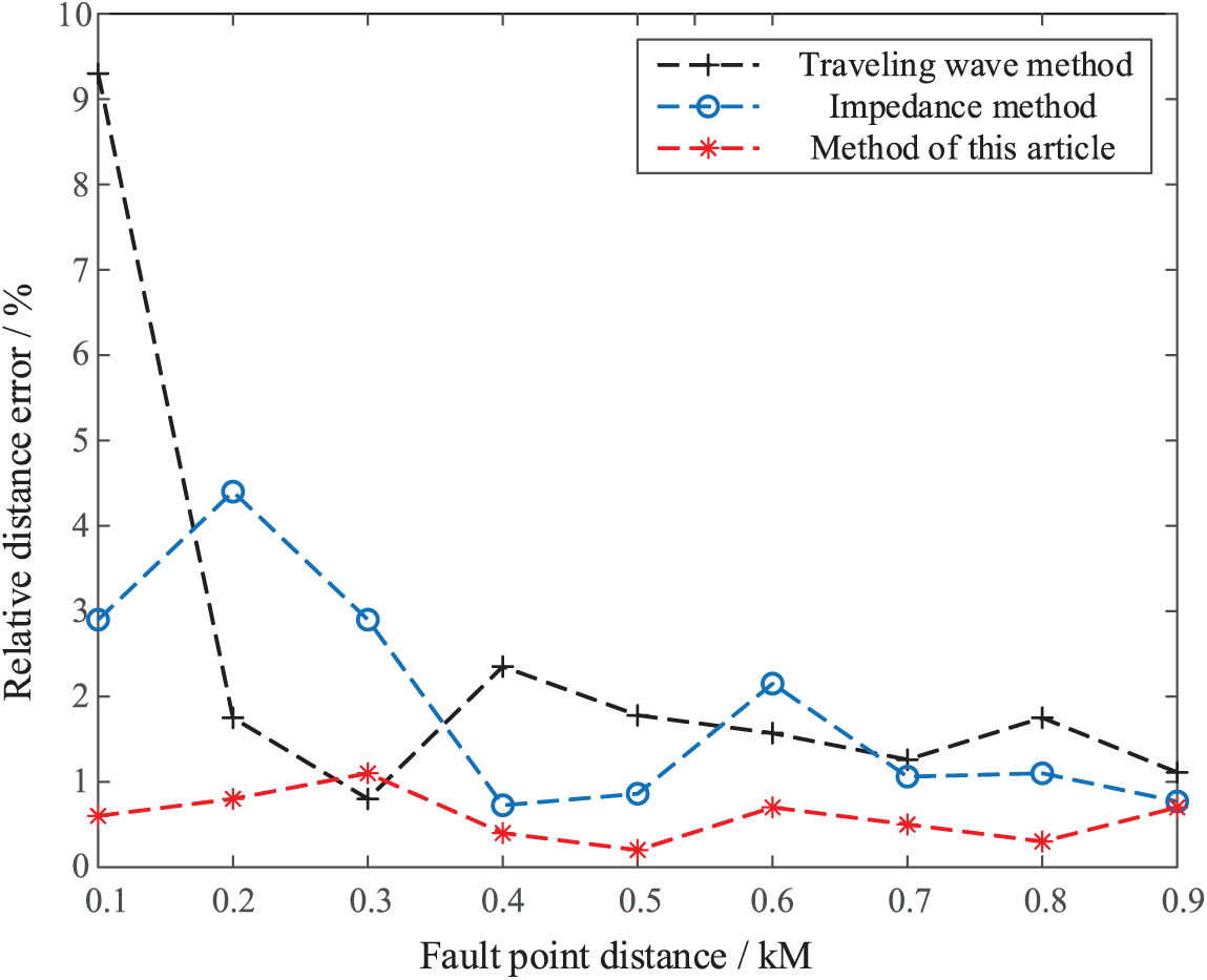
Figure 24: Relative error of different ranging methods

According to Table 5 and Fig. 24, the relative error of the fault location method proposed in this paper is mostly less than 1% in the fault location process, whereas the relative error of the impedance method and the traveling wave method is mostly around 2%, with the highest being 9.3%. As a result, the method proposed in this paper is more precise than the other two.

6  Conclusion

To address the difficulty of fault inspection in offshore wind farm collection systems, this paper proposes a fault location method for wind farm collection systems based on the λ-NIM dictionary and the J-CoSaMP algorithm, and simulates, verifies, and analyzes a 60-node wind farm collection system. This paper’s main contribution is as follows:

(1) The phase-locked loop trigonometric function method is used to extract the fault negative sequence voltage to form the node negative sequence voltage equation, suppressing the peak phenomenon and narrowing the gap between the read and actual voltage values.

(2) The compressed sensing theory is introduced, and the node impedance matrix is deduced further in the node voltage equation. The fault location coefficient creates the λ-NIM dictionary.

(3) The J-CoSaMP algorithm reconstructs the negative sequence current, and the fault location is realized by combining the voltage and impedance characteristics of the measuring point.

Funding Statement: This work was partly supported by the National Natural Science Foundation of China (52177074).

Conflicts of Interest: The authors declare that they have no conflicts of interest to report regarding the present study.

References

1. Ben, K. (2020). Wind energy beijing declaration developing 3 billion of wind power, leading green development and implementing the “30–60” target. Wind Energy, 11(5), 34–35. [Google Scholar]

2. Wang, B., Ren, X. (2021). Single-line-to-ground fault location in wind farm collection line with neutral point grounding with resistor. Proceedings of the CSEE, 41(6), 2136–2144. https://doi.org/10.13334/j.0258-8013.pcsee.200340 [Google Scholar] [CrossRef]

3. Zhai, Y. J., Zhang, K., Zhu, Y. L. (2020). Single-line-to-ground fault location method for wind farm collection line based on segmented impedance matching. Smart Power, 48(12), 26–32. [Google Scholar]

4. Zhang, K., Ma, C. X., Cao, Y. Q. (2020). Fault location based on parameter estimation in hybrid transmission lines of wind farm. Acta Energiae Solaris Sinica, 41(8), 323–329. https://doi.org/10.19912/j.0254-0096.2020.08.043j.0254-0096.2020.08.043 [Google Scholar] [CrossRef]

5. Pen, H., Zhu, Y. L., Yuan, S. (2020). Combined single-phase ground fault ranging for wind farm collector lines. Chinese Journal of Scientific Instrument, 41(9), 88–97. https://doi.org/10.19650/j.cnki.cjsi.J2005976 [Google Scholar] [CrossRef]

6. Hamidi, R. J., Livani, H. (2017). Traveling-wave-based fault-location algorithm for hybrid multiterminal circuits. IEEE Transactions on Power Delivery, 32(1), 135–144. https://doi.org/10.1109/TPWRD.2016.2589265 [Google Scholar] [CrossRef]

7. Wang, X. D., Wang, Y. C., Liu, Y. C. (2022). Fault location method for collector lines by combining decision coefficient and ESMD-TEO. Proceedings of the CSU-EPSA, 34(3), 51–58. https://doi.org/10.19635/j.cnki.csu-epsa.000845 [Google Scholar] [CrossRef]

8. Zhang, K., Zhu, Y. L., Ma, C. X. (2018). A new method for traveling wave ranging of transmission lines based on optimized traveling wave velocity. Journal of North China Electric Power University (Natural Science Edition), 45(4), 34–40. [Google Scholar]

9. Peng, H., Wang, W. H., Zhu, Y. L. (2021). Single-phase grounding intelligent ranging of wind farm collector line based on LSTM neural network. Power System Protection and Control, 49(16), 60–66. https://doi.org/10.19783/j.cnki.pspc.201457 [Google Scholar] [CrossRef]

10. He, Q., Pang, Y., Jiang, G., Xie, P. (2021). A spatio-temporal multiscale neural network approach for wind turbine fault diagnosis with imbalanced SCADA data. IEEE Transactions on Industrial Informatics, 17(10), 6875–6884. https://doi.org/10.1109/TII.2020.3041114 [Google Scholar] [CrossRef]

11. Wu, X., Jiang, G., Wang, X., Xie, P., Li, X. (2019). A multi-level-denoising autoencoder approach for wind turbine fault detection. IEEE Access, 7, 59376–59387. https://doi.org/10.1109/ACCESS.2019.2914731 [Google Scholar] [CrossRef]

12. Rezamand, M., Kordestani, M., Carriveau, R., Ting, D. S. (2020). A new hybrid fault detection method for wind turbine blades using recursive PCA and wavelet-based PDF. IEEE Sensors Journal, 20(4), 2023–2033. https://doi.org/10.1109/JSEN.2019.2948997 [Google Scholar] [CrossRef]

13. Yang, L., Zhang, Z. (2021). A conditional convolutional autoencoder-based method for monitoring wind turbine blade breakages. IEEE Transactions on Industrial Informatics, 17(9), 6390–6398. https://doi.org/10.1109/TII.2020.3011441 [Google Scholar] [CrossRef]

14. Dhiman, H. S., Deb, D., Muyeen, S. M., Kamwa, I. (2021). Wind turbine gearbox anomaly detection based on adaptive threshold and twin support vector machines. IEEE Transactions on Energy Conversion, 36(4), 3462–3469. https://doi.org/10.1109/TEC.2021.3075897 [Google Scholar] [CrossRef]

15. Lu, S., Gao, Z., Xu, Q. (2022). Class-imbalance privacy-preserving federated learning for decentralized fault diagnosis with biometric authentication. IEEE Transactions on Industrial Informatics, 18(12), 9101–9111. [Google Scholar]

16. Xu, Q., Lu, S., Jia, W. (2020). Imbalanced fault diagnosis of rotating machinery via multi-domain feature extraction and cost-sensitive learning. Journal of Intelligent Manufacturing, 31(6), 1467–1481. [Google Scholar]

17. Ge, Y. Z. (2007). The principle and technology of advanced relay protection and fault location. China: Xi’an Jiaotong University Press. [Google Scholar]

18. Jia, K., Feng, T., Zhao, Q. J. (2020). Bipolar short-circuit fault location of DC distribution network based on sparse measurement of fault high frequency voltage. Automation of Electric Power Systems, 144(1), 142–151. [Google Scholar]

19. Xu, G., Gong, Q. W., Li, X. (2014). Single-ended fault location method based on atomic decomposition and natural frequency of traveling wave. Automation of Electric Power Systems, 34(5), 133–138. [Google Scholar]

20. Yu, H. N., Ma, Q. Q., Wang, H. (2020). Fault location of VSC-HVDC transmission line based on compressed sensing. Acta Energiae Solaris Sinica, 41(3), 158–166. [Google Scholar]

21. Baraniuk, R. (2007). A lecture on compressive sensing. IEEE Signal Processing Magazine, 24(4), 118–121. [Google Scholar]

22. Lu, C., Liu, Y. H. (2015). RIP criterion in compressive sensing theory. Automation and Instruments, 190(8), 1001–9227. https://doi.org/10.14016/j.cnki.1001-9227.2015.08.211 [Google Scholar] [CrossRef]

23. Zhang, S. N., Luo, H. Y., Cheng, X. X. (2020). Realization of positive & negative sequence component picking up and phase locked loop using FPGA based on dual-dq transform. High Voltage Apparatus, 56(3), 182–189. https://doi.org/10.13296/j.1001-1609.hva.2020.03.027 [Google Scholar] [CrossRef]

24. Wang, K., Wu, Y. M., Zhuge, J. C. (2019). MsGOMP infrared image denoising algorithm based on generalized jaccard coefficient. Infrared Technology, 41(6), 577–584. [Google Scholar]

25. Li, Z. X., Tian, B., Li, Z. H. (2016). Two-terminal nonsynchronized fault location algorithms for single/double transmission lines. Automation of Electric Power Systems, 40(22), 105–110. [Google Scholar]