The Short-Term Prediction of Wind Power Based on the Convolutional Graph Attention Deep Neural Network

1  Introduction

Wind energy is the world’s third-largest renewable energy source with huge development potential. China has the world’s largest installed capacity [1]. However, wind energy is affected by atmospheric movement and its changes have strong randomness and volatility. With the development of built-in monitoring and data acquisition technology in power systems, wind farms have stored a large amount of historical wind power data and meteorological data that can be used for wind power prediction [2].

1.1 Related Literature Review

After the research and development of wind power prediction technology over many years, a large number of prediction models have been proposed. These models can be divided into three categories according to the prediction techniques, namely the statistical model, the machine learning model, and the deep learning model [3]. A typical statistical model is the time series model, such as the autoregressive [4] and autoregression moving average [5], etc. The machine learning model includes multilayer perceptron [6], support vector machine [7], random forest [8], etc. However, it is difficult for traditional machine learning prediction models based on shallow networks to handle complex and multi-source historical data. Deep learning models have strong feature extraction ability and generalization abilities [9]. In the field of wind power prediction, the relatively mature deep learning networks are the CNN [10,11] and recurrent neural networks represented by LSTM [12,13] and GRU [14,15]. CNN is widely used to extract non-linear features in complex sequences, and LSTM and GRU are suitable for times series data modeling [16].

Numerical weather prediction data include the wind speed, the wind direction, the humidity, and other prediction data related to wind power [17]. Selecting appropriate NWP data as the feature input, many deep learning models can show better performance in wind power prediction. However, the complex and diverse NWP data related to wind power can diminish the prediction models’ performance, so the dynamic features of NWP data need to be extracted by efficient methods [18]. Literature [19] proposed a wind power probabilistic prediction model based on CNN and verifies its accuracy. In Literature [20], CNN and physical models are combined in prediction, which further improves the forecasting efficacy of short-term wind power. Considering the effect of meteorological elements on wind power forecasting, literature [21] screened the multivariate meteorological information data highly correlated with wind power with distance analysis and uses it as the LSTM model’s input data. The hybrid model composed of CNN and LSTM can take advantage of each model, further improving the forecasting performance [22]. Literature [22] combined CNN and LSTM for wind power prediction and takes into consideration the meteorological elements’ influence on wind power in time and space.

Wind power is essentially determined by meteorological factors with spatial-temporal characteristics, including the wind speed and the wind direction. Conventional input features of wind power forecasting are all the relevant datasets of the local wind farm, which can only capture the features in time series and ignore the spatial-temporal features [23]. With the improvement of the electric system measurement system, the meteorological data of different wind farms can be managed centrally. Therefore, algorithms could be used to fuse and extract features of the data of adjacent wind farms, and to achieve more accurate wind power prediction [24]. However, deep neural networks such as CNN are mainly used to deal with well-structured data. However, the wind farm location distribution, in reality, is irregular. Therefore, it is more reasonable to use the graph structure to characterize the relationship between each wind farm. Based on the graph structure, each wind farm is independent and connected by the line relationship. For such graph structure data, graph neural networks [25] (GNN) have relatively good spatial-temporal feature extraction effects. Literature [26] proposed a graph deep learning model, which is used to study neighboring wind farms’ spatial-temporal characteristics from the wind speed and wind direction data, and to forecast the wind speed of the entire graph node according to the extracted spatial-temporal characteristics. In literature [27], the spatial-temporal correlation graph neural network was proposed to forecast the multi-node offshore wind speed, to better capture the potential spatial dependency from node relationships and historical time series, and to distinguish node contributions and generate high-dimensional spatial characteristics.

At present, GNN-related research is developing rapidly, among which the graph convolutional neural network [28] (GCN) has been studied and applied in many fields. GCN depends on the initial adjacency matrix and the graph attention network [29] introduces the attention mechanism based on GCN. Compared with GCN, an adaptive edge weight coefficient is added to the graph attention layer of GAT. The weight coefficient matrix of GAT does not require complex data formulas, and it can be automatically learned from GAT. In addition, the attention mechanism reduces the number of parameters to be learned. Therefore, the graph attention model has very efficient graph data processing and expression performance compared with GCN.

1.2 Contributions of This Work

All the above models are point prediction models, which obtain the deterministic value of the future wind power but cannot accurately describe the uncertainty of the wind power. Due to the strong volatility of wind electricity power, point forecasting may not be reliable enough to satisfy realistic scheduling needs [30]. As a result, the probability and interval forecasting of wind power has become a research hot topic. In literature [31], the authors designed a multi-source and temporal attention model to dynamically select the variables of NWP and extract temporal dependency, and construct a multi-step probabilistic prediction using a mixture density module based on a beta kernel. However, this study only considers temporal dependency. Literature [32] developed a method that improves short-term wind power probabilistic prediction by the combination of deep belief network (DBN), error scenario partitioning method that is used to mine spatial-temporal dependence of NWP data, and kernel density estimation. However, the proposed method is affected by the power characteristic curve’s accuracy. The interval prediction can provide a high-confidence prediction interval and the probability forecasting can fit the probability density function curve of the forecasting result [33]. The interval forecasting and probability forecasting are usually implemented by a combined model of quantile regression (QR) and point prediction model [34]. Literature [35] combined QR with LSTM to propose a quantile regression long short-term memory model (QRLSTM) which obtains relatively accurate results for the wind power point prediction and the probability density prediction.

Based on existing research, a wind power probability forecasting model based on spatial-temporal feature extraction is proposed in the paper to realize accurate point prediction and reliable interval forecasting and probability forecasting of wind power. Firstly, CNN, GAT and attention mechanism are combined to extract the complex dynamic spatial-temporal characteristics of each adjacent wind farm. Then, LSTM is to build a QR prediction model to realize wind power forecasting. Finally, the wind power probability density function curve is obtained through KDE. The actual wind power data of a wind farm in the U.S. is tested and compared with other prediction models. As can be seen from the results, the forecasting efficacy of the proposed model has been improved. The main contributions of this work include the following threefold:

(1) Since the meteorological data comes from multiple wind farms, this paper combines CNN and GAT to extract characteristics of meteorological data. CNN is used to extract the complex dynamic temporal features of each adjacent wind farm, and the processed features are aggregated into the graph structure data, and then the GAT module is to learn the spatial-temporal features. Moreover, the multi-head attention mechanism is introduced in GAT to further overcome the complex data noise of meteorological data in the graph. Compared with other methods, the proposed model not only considers the meteorological data characteristics of the target wind farm, but also fuses the historical meteorological characteristics of multiple nearby wind farms for spatial-temporal feature extraction, which fully considers the coupling relationship between wind power and multi-source meteorological factors, and improve the prediction accuracy of wind power.

(2) We combined LSTM and QR to construct a wind power prediction model, and realized point and probabilistic wind power forecasting based on spatial-temporal data of multi-wind fields.

(3) The actual wind farm data is used for example test, and the comparison experiment with several models is carried out to verify the superiority of the proposed CGA-LSTM model. In addition, for the purpose of ensuring the reproduction of the proposed prediction method, we published the relevant code on GitHub1.

2  The Algorithm Model Principle

2.1 The Graph Modeling

The research subject of GAT is graph data, which is modeled from graph theory. The graph here refers to the data structure similar to the topological graph which consists of nodes and edges. The formula of the graph is given by:

G=(V,E,A)V={v|v∈dataobject}E={<v,w>|v,w∈V∧p(v,w)}(1)

wherein V represents the set of vertices, E represents the set of lines, and A represents the adjacency matrix of graphs. The elements in the adjacency matrix only represent the connection relation between wind farms. Therefore, the adjacent matrix of GAT is constructed as follows:

Aij={1PCC(vi,vj)≥γ0PCC(vi,vj)<γ(2)

wherein PCC(vi,vj) indicates the Pearson correlation coefficient of the ith and the jth wind farm meteorological data. When PCC(vi,vj) is greater than or equal to γ, vi and vj are linked to the edge eij∈E with a weight of 1. When PCC(vi,vj) is less than γ, vi and vj are not linked with edges, indicating that only the influence between connected points is considered in the attention mechanism application.

2.2 The Graph Attention Network GAT

The main principle of GAT is that in the model parameter training and feature extraction of graph data, the neighborhood weight of the target node and its adjacent nodes is determined by the attention mechanism. In this way, the spatial-temporal correlation between nodes can be determined by the edge weight without depending on the initial adjacent matrix.

Fig. 1 shows the framework of GAT, h1 denotes the meteorological data of the target wind farm station, h2∼h6 denote the meteorological data of the nearby station, w1 constitutes the weight matrix W, and h1′ represents the output of the target wind farm station. The GAT input can be expressed as:

h={h→1,h→2,…,h→N},h→i∈RF(3)

wherein N represents the quantity of nodes and h→ denotes the input of a single node.

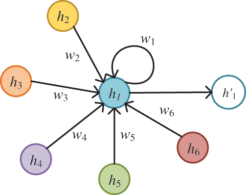
Figure 1: The structure of GAT

Each node in GAT corresponds to a hidden state. The hidden state is jointly determined by the data input of its node and the relevant influence of the neighbor node data. This process is mainly realized through the self-attention mechanism. Its attention coefficient is calculated as follows:

eij=a(Whi,Whj)(4)

wherein eij is the attention coefficient of the adjacent node j to the target node i. hi and hj represent the hidden state of the adjacent nodes. W is the weight matrix and a(⋅) is the attention mechanism, indicating the correlation between feature vectors.

It can avoid the relatively large calculation amount by calculating only the attention correlation coefficient of the target node i and its adjacent node j. Its expression is as follows:

αij=softmaxj(eij)=exp⁡(eij)∑k∈Niexp⁡(eik)(5)

wherein softmaxj(⋅) is the normalization function and Ni indicates the quantity of adjacent nodes of node i. And the nonlinear activation function LeakyReLU(⋅) is used for activation with the slope of 0.2.

αij=exp⁡(LeakyReLU(a→T[Wh→i∥Wh→j|]))∑k∈Niexp⁡(LeakyReLU(a→T[Wh→i∥Wh→k|]))(6)

wherein ∥ indicates the feature connection and a→T[Wh→i∥Wh→j|] shows that nodes i and j are feature-extracted separately and stitched.

Through the above computation, the output of each node is obtained as follows:

h→i′=σ(∑j∈NiαijWh→j)(7)

wherein σ(⋅) represents the activation function of sigmoid and h→i′ denotes the output of node i.

Through GAT, the target node highly aggregates the characteristics information of each adjacent node according to the weight information with each adjacent node and adaptively extracts the highly correlated node features of adjacent nodes. Therefore, GAT has efficient spatial-temporal feature extraction ability and GAT is flexible in modeling without relying on the graph structure and node order, which can enhance the model’s prediction ability.

2.3 The Head Attention Mechanism

To raise the reliability and stability of GAT spatial-temporal feature extraction, we bring the multi-head attention mechanism to GAT. The multi-head attention uses K independent attention mechanisms to improve formula (7), that is, the K-order parallel independent operation of GAT is conducted. Then, the results of each conversion are combined to obtain the final feature output result as follows:

h→i′=||k=1Kσ(∑j∈NiαijkWkh→j)(8)

wherein αijk represents the normalized result of the attention coefficient αk of the kth order attention mechanism. The features of each head are connected or averaged to get the final feature output h1′→.

The graph data, especially when there is complex data noise in the meteorological data, will greatly impact the performance of GAT. However, the multi-head attention mechanism can make GAT mode’s attention learning more reliable and stable, which can help notice the most important node in the graph and highlight the most important feature information.

2.4 The Convolutional Neural Network CNN

CNN is a deep neural network on the basis of convolution operation with pooling, local connection, and weight sharing. It is widely used to automatically learn labeled data and extract complex features in data [11]. The structure of the one-dimensional CNN is displayed in Fig. 2, which is mainly composed of two convolution layers, two pooling layers, and one fully connected layer. Features of the input data are extracted by the convolutional layer through scanning the convolution core. The pooling layer is utilized to sample the features that are extracted by the convolution layer, and to reduce network complexity while retaining the feature vector’s main information; the fully-connected layer is to select the appropriate activation function for full connection, and the output activation value is the feature extracted by CNN.

Figure 2: The structure of one-dimensional CNN

2.5 The Long Short-Term Memory LSTM

Based on recurrent neural network (RNN), the LSTM model has been improved and solved RNN’s problem of being unable to effectively process long-distance information and being prone to gradient disappearance and explosion. Therefore, it is widely used in the analysis and processing of time series data. As shown in Fig. 3, the unit structure of LSTM mainly contains the “forget gate”, the “input gate”, and the “output gate”, whose outputs are ft, it and ot, and can selectively retain or forget information, thus overcoming the adverse effects of short-term memory. The forget gate is to decide what information should be discarded or retained. The input gate is to update the cell state and selectively transmits the formerly hidden status information and new input information to the new LSTM cell, and the output gate is used to regulate the filtering of the unit cell status and determine information of the next hidden state. In addition, xt denotes the input of the LSTM unit, ct−1 and ct denote the cell unit states of the previous moment and the current moment, respectively, and ht−1 and ht denote the corresponding hidden layer states.

Figure 3: The unit structure of LSTM

3  The Wind Power Prediction Model Based on CGA-LSTM

3.1 CGA-LSTM Model

As shown in Fig. 4, the multi-wind farm wind power spatial-temporal prediction combined model CGA-LSTM consists of the input module, the spatial-temporal feature extraction module, the deep learning prediction module, and the output module. The input module includes the meteorological data of multiple wind fields X1,X2,⋯,Xn whose temporal characteristics are extracted by CNN, and the wind power historical data XP. The feature extraction and deep learning module are the core of the model, which jointly achieved accurate and reliable prediction of wind power. Through introducing the multi-head attention mechanism into GAT layers, the spatial-temporal feature extraction module mines the spatial-temporal characteristics of meteorological data from different wind farms to prepare for further wind power forecasting. The deep learning prediction module is composed of LSTM, which further achieves the effective correlation between the spatial-temporal characteristics of meteorological data and wind power data. The forecasting model based on CGA-LSTM realizes wind power characteristics mining through the above two modules, and obtains point and probability forecasting results through the output module. Next, the specific functions of each module are introduced, respectively.

Figure 4: The structure of CGA-LSTM

3.1.1 Input Module

The model has two input modules, the meteorological data of n adjacent wind farms Xnwp=[X1,X2,…,Xn] and the wind power historical data input XP stitched together with the spatial-temporal features extracted from GAT.

The meteorological data mainly include the wind speed, the wind direction, the atmospheric density, the humidity, and the temperature. The correlation and dimension between the meteorological data are different, and the time series features of wind power are not obvious. Therefore, to guarantee the more efficient spatial-temporal feature extraction of the subsequent GAT layer, an independent convolution-based feature extraction module is used for the meteorological data of each node to initially extract the high-dimensional dynamic time series feature of each node. The meteorological data of each node Xfi is transformed into a one-dimensional time series feature Xf=[Xf1,Xf2,…,Xfn] through convolution, pooling, flattening, and other operations. The node data of the graph data is composed of n time series features. As the input of each graph network node, the time series feature Xf of each node obtained by convolution constitutes an undirected fully connected graph, which is the input of the GAT network.

3.1.2 The Spatial-Temporal Feature Extraction Module

The spatial-temporal feature extraction module has three parallel independent GAT modules, and each GAT module consists of two GAT layers, which is to extract the spatial-temporal characteristics of the target node. The multi-head attention mechanism is utilized to make the prediction effect more stable and reliable. The fusion feature is obtained by adjusting the dimension of XG and XP.

3.1.3 Deep Learning Prediction Module

In the probability prediction module, LSTM is used to extract the fusion feature XF. The results are processed by the multi-fully connected layer. The quantile loss function optimization training is received and the wind power’s predicted value under diverse quantiles is finally output. The quantile loss function is:

min1mq∑j=1q∑i=1mρτj(yi−f(W(τj),b(τj),Xi))(9)

wherein m denotes the number of samples for each batch training set. q is the number of quantiles. yi represents the real value of the output. Xi represents the input of the sample. f(W(τj),b(τj),Xi) is the predicted value output by the ith sample of under the quantile condition τj. W(τj) and b(τj) denote the model parameters related to the quantile τj. f(⋅) is the nonlinear function that reflects the connection between X and y. ρ(⋅) is the check function and its formula is as follows:

ρτ(μ)=μ(τ−I(μ)),I(μ)={1,μ<00,μ≥0(10)

wherein is the indicator function and μ is the input of the function.

The process of the probability prediction module can be calculated as:

y~(τ)=f(W~(τ),b~(τ),XF)(11)

wherein y~(τ) is the wind power predicted value at the quantile τ. W~(τ) and b(τ) are the network weight and deviation, respectively. XF denotes the fusion feature. And y~(τ) denotes the predicted output of wind power.

3.1.4 The Output Module

Based on the predicted values of different quantile conditions, the point and interval forecasting results can be obtained. The point prediction result is the predicted value y~(0.5) at the of 0.5. The interval prediction is [y~(τdown),y~(τup)], wherein τdown and τup represent the confidence interval lower and upper limits at the given confidence degree. The prediction results of different quantile conditions at a certain time can be seen as a random sample following a certain distribution. Therefore, KDE can fit all the quantile predicted values at that time to get the PDF of the wind power predicted value at that time.

The KDE expression is as follows:

gh(z)=1nh∑i=1nK(z−zih)(12)

wherein gh(z) represents the estimated PDF. n denotes the number of samples. K(⋅) represents the kernel function. h is the kernel function bandwidth. Epanechnikov is selected as the kernel function. In this paper, we select the grid search with cross-validation to obtain the suitable bandwidth.

3.2 Evaluation Indicators to Predict Model Performance

3.2.1 Point Prediction Evaluation Indicators

To assess and compare the point prediction capability of the forecasting model, the root mean square error (RMSE) and normalized mean absolute percentage error (NMAPE) are adopted as the evaluation metrics with the formulas as:

ERMSE=1n∑i=1n(yi−y^i)2(13)

ENMAPE=1n∑i=1n|yi−y^i|maxi=1nyi×100%(14)

wherein n denotes the quantity of test samples. i denotes the sample serial number. yi and y^i represent the real value and predicted value of the ith sample output, respectively.

The model with the smaller RMSE and NMAPE values has higher point forecasting accuracy.

3.2.2 Probabilistic Prediction Evaluation Indicators

To assess the effect of interval prediction models, we selected the average coverage error (ACE), the prediction interval normalized average width (PINAW), and the interval sharpness (IS) metrics for comparative analysis. The formula is:

EACE=(1n∑i=1n{1,yi∈[liα,uiα]0,yi∉[liα,uiα]−(1−α))×100%(15)

EPINAW=1ns∑i=1n(uiα−liα)(16)

EIS=1n∑i=1n{−2α(uiα−liα),yi∈[liα,uiα]−2α(uiα−liα)−4(liα−yi),yi<liα−2α(uiα−liα)−4(yi−uiα),yi>uiα(17)

wherein α represents the significance level. uiα and liα represent the lower and upper limits of the ith sample prediction under confidence degree (1−α). s is the difference value of the actual maximum and minimum value.

A larger ACE indicates a larger coverage of the prediction interval at a certain significance level and a higher interval prediction reliability. Smaller PINAW indicates the narrower average width of the prediction interval obtained by the model. And higher IS indicates the better interval prediction comprehensive capability of the model.

In this paper, the continuously ranked probability score (CRPS) is employed to reflect the probability forecasting efficacy. And the formula is as follows:

ECRPS=1n∑i=1n∫−∞+∞[F(yi)−I(y^i−yi)]2dyi(18)

F(yi)=∫−∞yip(xi)dxi(19)

wherein i is the sample serial number. F(⋅) represents the cumulative density function; xi denotes the i sample input. And p(⋅) denotes the probability density function. Smaller CRPS indicates the better probability prediction comprehensive capability of the model.

4  The Example Test

To confirm the proposed model’s forecasting effect, the wind power historical data and meteorological data of Rock River Wind Farm from January 01, 2012 to December 31, 2012, including the wind speed, the wind direction, the temperature, and the humidity are adopted. The meteorological data of 10 adjacent wind farms are selected by the Pearson’s correlation coefficient method. The data is 1 recording point per hour. Compared with other meteorological data, the correlation of wind speed and wind power data is the strongest. As shown in Fig. 5, the higher the wind speed, the greater the corresponding wind power output, but the relationship between them is nonlinear, and when the wind speed reaches a certain point, the power output of the fan will tend to be stable. The relevant characteristics of other meteorological data and wind power are relatively complex, and the proposed method can learn the dynamic complex characteristics well to achieve the forecast target.

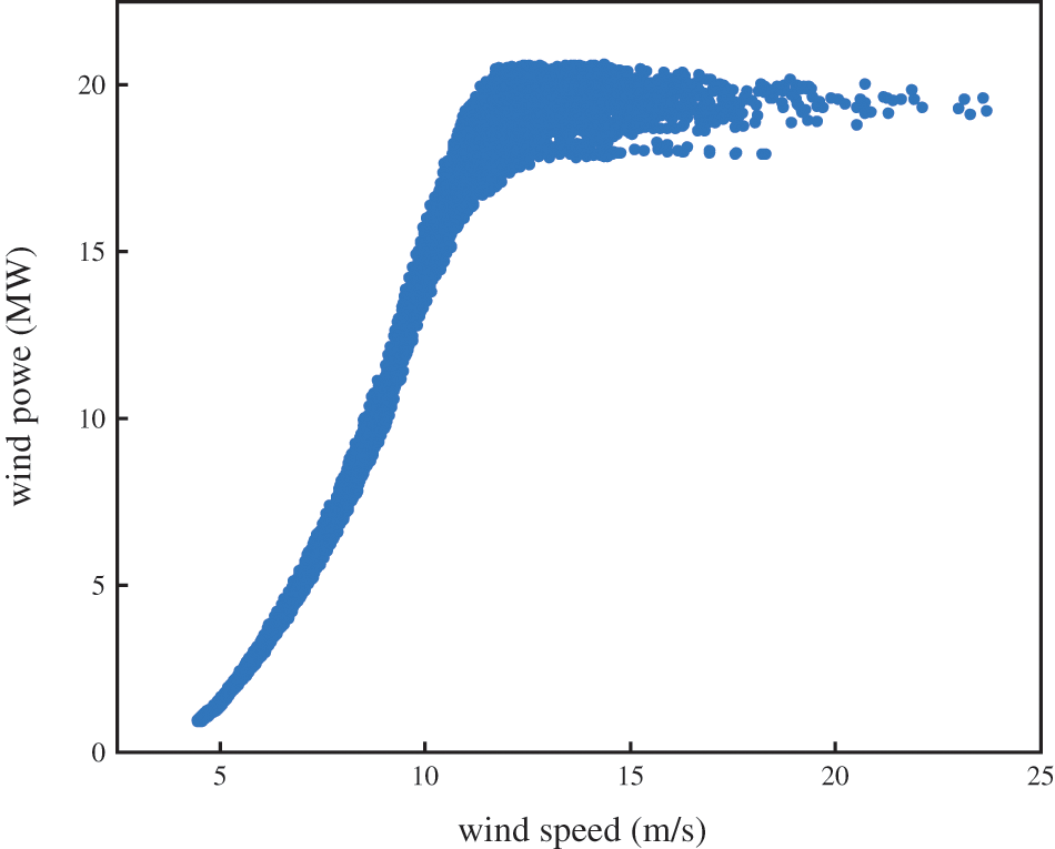
Figure 5: The target site wind speed and wind power data scatter plot

4.1 The Input Data Normalization

To prevent the neuron saturation, the normalized input data is required. In this paper, the min-max normalization method is adopted with the expression as:

x^=xmax−xxmax−xmin(20)

wherein x^ denotes the normalized data. x denotes the original data. And xmax and xmin denote the maximum and minimum value of the original data, respectively.

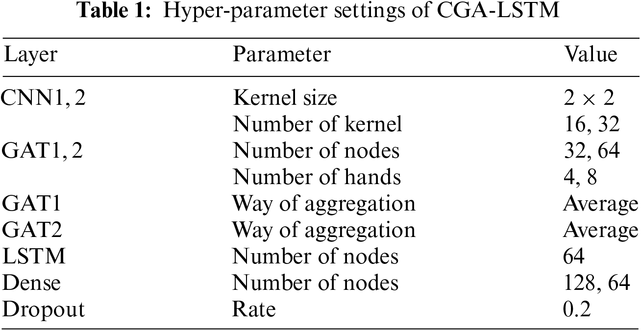
4.2 The Model Parameter Setting

The proposed model sets 99 quantile points with the quantile point τ = [0.01, 0.02, …, 0.98, 0.99]. Table 1 displays the hyper-parameter settings of the CGA-LSTM model. To demonstrate the superior comprehensive spatial-temporal prediction performance of CGA-LSTM, GCN-LSTM, CNN-LSTM, CGA-MLP and LSTM are selected as the comparison models. GCN-LSTM could process the graph network data. It has the same structure set up as the CGA-LSTM but requires the input of the initial adjacent matrix. CNN-LSTM and LSTM cannot process the graph network data. Therefore, their input is only the meteorological datasets of the targeted wind farm and the structure is cascaded. The CGA-MLP model consists of a CGA module and a fully connected layer (MLP) as a measure of the necessity of LSTM networks. Next, the efficacy of the proposed model and others in the point prediction and probabilistic prediction are compared, respectively.

4.3 The Analysis of Prediction Results

4.3.1 The Analysis of the Point Prediction Effect

In the paper, the predicted value corresponding to 0.5 quantiles of each model is selected as the wind power point forecasting result. Table 2 shows the point prediction result error statistics for each model. As can be seen in Table 2, RMSE and NMAPE of CGA-LSTM are the lowest. Compared with other models, RMSE decreases by 0.0741, 0.3035, 0.3732, and 0.3865 MW, respectively, and NMAPE decreases by 0.3133%, 1.1391%, 1.4554%, and 1.548%, respectively. Table 2 also indicates that each component of the model contributes to the overall performance and removing any component would lead to a significant drop in the performance. The prediction accuracy of the models using the graph network to extract spatial-temporal features is higher than those using the single wind farm data. Compared with the effect of CGA-LSTM, the wind power prediction accuracy of CGA-LSTM is the highest, indicating that the proposed CGA module is effective in processing spatial-temporal features.

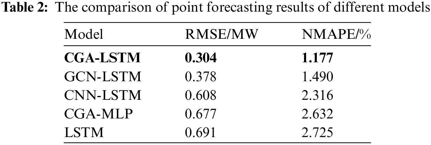
Fig. 6 is the comparison between the predicted value of each model and the actual value of wind power. As displayed in Fig. 6, relying on the performance of deep learning, each model has good point prediction performance. However, by comparing the randomly selected magnified sub-graphs, it can be seen more clearly that the predicted value of the CGA-LSTM model is closest to the real value. To summarize, the CGA-LSTM model has better point forecasting performance of short-term wind power.

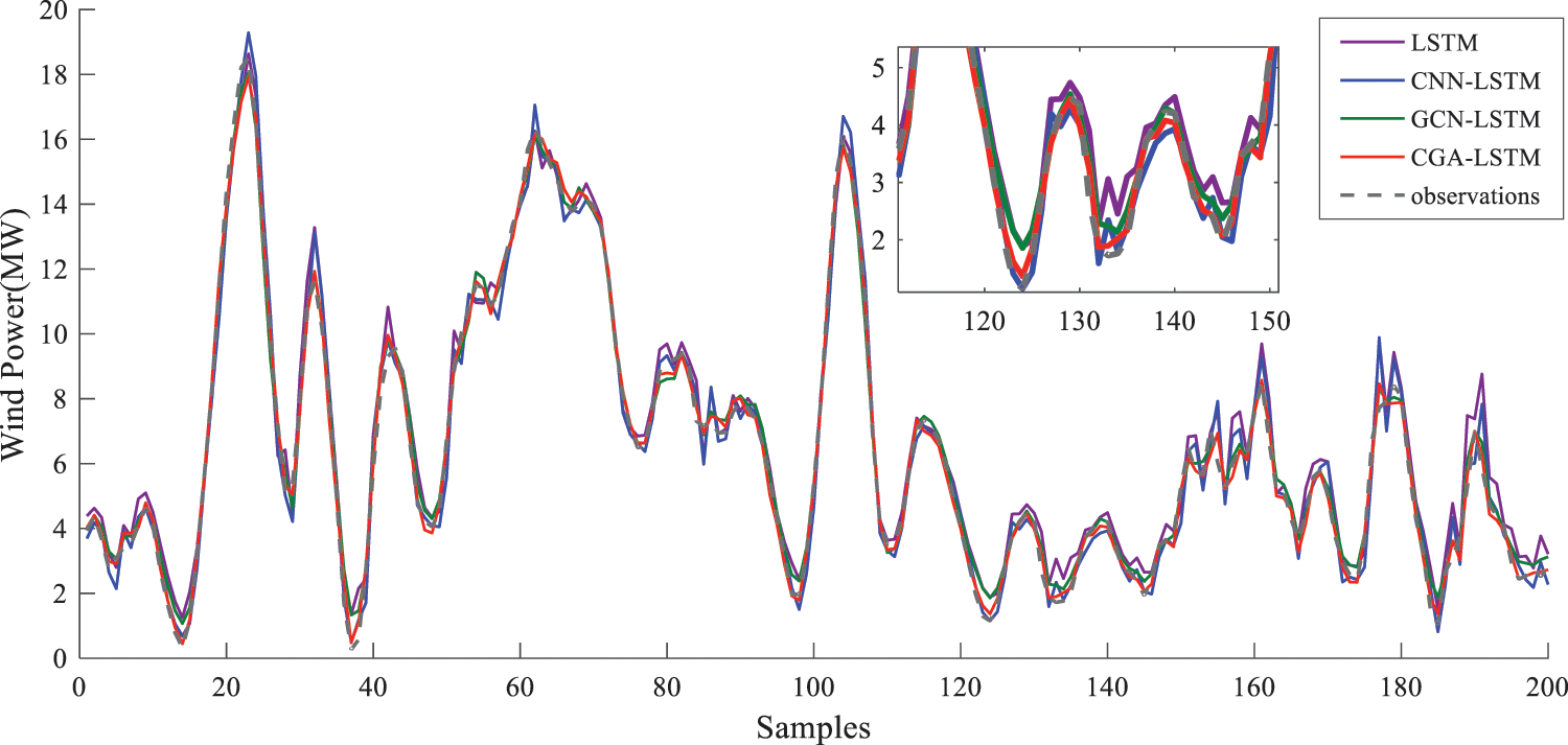
Figure 6: Point forecasting results of diverse models

4.3.2 The Analysis of Probability Prediction Effect

The forecasting results at diverse quantiles are gained from CGA-LSTM by using QR. The KDE method was utilized to fit the PDF for each observation point, and Fig. 7 displays the PDF of 4 randomly selected observation points. As can be seen from Fig. 7, most of the real values approach the PDF peak and the predicted median, which indicates the proposed probability forecasting model is efficient.

Figure 7: The PDF curve at different observation points predicted by CGA-LSTM

The error statistics of each model’s probabilistic forecasting are shown in Table 3. It can be concluded that:

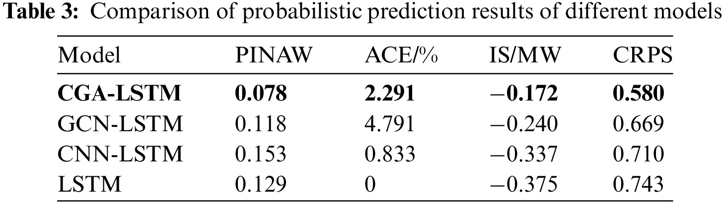
First, the ACE average value of CGA-LSTM and all contrast models is no less than 0, indicating that the models’ prediction interval meets 95% confidence.

The IS and CPRS values of CGA-LSTM are the lowest. The IS absolute value of CGA-LSTM decreases by 0.0674, 0.1649, and 0.2027, respectively. In comparison with other models, the CPRS value of CGA-LSTM decreases by 0.0886, 0.1295, and 0.1631, respectively. It means that CGA-LSTM has narrower prediction intervals and higher acuity, interval prediction comprehensive performance, and probabilistic prediction performance. Based on the above analysis, the CGA-LSTM model proposed in this paper is effective in using spatial-temporal features for probabilistic prediction.

In order to illustrate that CGA-LSTM proposed in this work can better describe the uncertainty of wind power prediction, Fig. 8 shows the interval forecasting results of diverse models in the same period. It is obvious that the actual value of CGA-LSTM almost all falls within its prediction interval, which indicates that the performance of CGA-LSTM in interval prediction is very reliable. In addition, the figure shows that the proposed model is narrower in the prediction interval compared with contrast models, indicating that the proposed model CGA-LSTM has relatively high interval prediction acuity.

Figure 8: Interval forecasting results of diverse models

For the purpose of further illustrating the proposed method prediction effectiveness, we also select three methods for comparative experiments, namely SATCN-LSTM [36], TAC-BiLSTM [37] and SANN [38]. The evaluation indexes of point prediction and interval prediction results for the 90% confidence interval of different models are shown in Table 4. It can be seen that the proposed model obtains optimal results on each evaluation index. For point prediction, compared with other models, RMSE and NMAPE of CGA-LSTM are the lowest, which are reduced by 11.8% and 1.1% on average, respectively, which reflects that the feature extraction model CGA can give full play to its own performance, and actively enhance the point prediction accuracy. For interval prediction, under the 90% confidence level, although the absolute values of ACE of CGA-LSTM is not the smallest, PINAW and the absolute values of IS are both the smallest, indicating that the prediction interval generated by this method has good reliability, higher sensitivity and better comprehensive performance. In summary, the method of this paper has certain advantages over other selected methods, especially in the scenario of multiple wind field data, where the proposed model can fully consider the coupling relationship between wind power and meteorological factors, and obtain better prediction results.

5  Conclusion

In this paper, a wind power prediction model of convolution graph attention long short-term memory model based on multi-wind farm spatial-temporal data, namely CGA-LSTM, has been proposed. Firstly, CNN is used to primarily extract the high-dimensional characteristics of the meteorological data at each node. Then, the multi-layer attention network is used to extract the spatial-temporal characteristics of the graph data and LSTM is combined to form the graph attention deep neural network CGA-LSTM, which can effectively extract the spatial-temporal characteristics of the multi-wind farm meteorological data and realize the deterministic and probabilistic prediction of wind power using multi-wind farm meteorological data. Compared with traditional models such as CNN-LSTM, the proposed model has a higher prediction capability. The proposed model has only one target node, that is, the multi-wind farm meteorological data is used to predict the wind power of only one wind farm. In future research, multi-task models can be constructed to predict and model multiple adjacent wind farms simultaneously and share the same graph network information.

Acknowledgement: Not applicable.

Funding Statement: This work was supported by the Science and Technology Project of State Grid Corporation of China (4000-202122070A-0-0-00).

Author Contributions: The authors confirm contribution to the paper as follows: study conception and design: Fan Xiao, Ping Xiong; data collection: Chang Ye; analysis and interpretation of results: Yusen Xu, Yeyang Li, Yiqun Kang; draft manuscript preparation: Dan Liu, Nianming Zhang. All authors reviewed the results and approved the final version of the manuscript.

Availability of Data and Materials: Due to some confidentiality and intellectual property issues, we are not able to provide relevant data.

Conflicts of Interest: The authors declare that they have no conflicts of interest to report regarding the present study.

1GitHub project website: https://github.com/liyeyang-isfj/CGA-LSTM.

References

1. Global Wind Energy Council (GWEC) (2022). Global wind report 2022. https://gwec.net/global-wind-report-2022 (accessed on 16/10/2023) [Google Scholar]

2. Jin, H. P., Shi, L. X., Chen, X. G., Qian, B., Yang, B. et al. (2021). Probabilistic wind power forecasting using selective ensemble of finite mixture Gaussian process regression models. Renewable Energy, 174, 1–18. [Google Scholar]

3. Zhou, M., Wang, B., Guo, S. D., Watada, J. (2021). Multi-objective prediction intervals for wind power forecast based on deep neural networks. Information Sciences, 550, 207–220. [Google Scholar]

4. Erdem, E., Shi, J. (2011). ARMA based approaches for forecasting the tuple of wind speed and direction. Applied Energy, 88(4), 1405–1414. [Google Scholar]

5. Amini, M. H., Kargarian, A., Karabasoglu, O. (2016). ARIMA-based decoupled time series forecasting of electric vehicle charging demand for stochastic power system operation. Electric Power Systems Research, 140, 378–390. [Google Scholar]

6. Ren, C., An, N., Wang, J. Z., Li, L., Hu, B. et al. (2014). Optimal parameters selection for BP neural network based on particle swarm optimization: A case study of wind speed forecasting. Knowledge-Based Systems, 56, 226–239. [Google Scholar]

7. Yu, C. J., Li, Y. L., Bao, Y. L., Tang, H. J., Zhai, G. H. (2018). A novel framework for wind speed prediction based on recurrent neural networks and support vector machine. Energy Conversion and Management, 178, 137–145. [Google Scholar]

8. Demolli, H., Dokuz, A. S., Ecemis, A., Gokcek, M. (2019). Wind power forecasting based on daily wind speed data using machine learning algorithms. Energy Conversion and Management, 198, 111823. [Google Scholar]

9. Zang, H. X., Cheng, L. L., Ding, T., Cheung, K. W., Wei, Z. N. et al. (2020). Day-ahead photovoltaic power forecasting approach based on deep convolutional neural networks and meta learning. International Journal of Electrical Power & Energy Systems, 118, 105790. [Google Scholar]

10. Oh, B. K., Glisic, B., Kim, Y., Park, H. S. (2019). Convolutional neural network-based wind-induced response estimation model for tall buildings. Computer-Aided Civil and Infrastructure Engineering, 34, 843–858. [Google Scholar]

11. Huang, R. M., Wang, X. H., Fei, F., Li, H. E., Wu, E. Q. (2022). Forecast method of distributed photovoltaic power generation based on EM-WS-CNN neural networks. Frontiers in Energy Research, 10, 902722. [Google Scholar]

12. Wang, F., Xuan, Z. M., Zhen, Z., Li, K. P., Wang, T. Q. et al. (2020). A day-ahead PV power forecasting method based on LSTM-RNN model and time correlation modification under partial daily pattern prediction framework. Energy Conversion and Management, 212, 112766. [Google Scholar]

13. Yuan, X. H., Chen, C., Jiang, M., Yuan, Y. B. (2019). Prediction interval of wind power using parameter optimized Beta distribution based LSTM model. Applied Soft Computing, 82, 105550. [Google Scholar]

14. Kisvari, A., Lin, Z., Liu, X. L. (2021). Wind power forecasting–A data-driven method along with gated recurrent neural network. Renewable Energy, 163, 1895–1909. [Google Scholar]

15. Niu, Z. W., Yu, Z. Y., Tang, W. H., Wu, Q. H., Reformat, M. (2020). Wind power forecasting using attention-based gated recurrent unit network. Energy, 196, 117081. [Google Scholar]

16. Wang, Y. Y., Wang, T. Y., Chen, X. Q., Zeng, X. J., Huang, J. J. et al. (2022). Short-term probability density function forecasting of industrial loads based on ConvLSTM-MDN. Frontiers in Energy Research, 10, 891680. [Google Scholar]

17. Wu, Y. K., Wu, Y. C., Hong, J. S., Phan, L. H., Phan, Q. D. (2021). Probabilistic forecast of wind power generation with data processing and numerical weather predictions. IEEE Transactions on Industry Application, 57(1), 36–45. [Google Scholar]

18. Yin, H., Ou, Z. H., Fu, J. J., Cai, Y. F., Chen, S. et al. (2021). A novel transfer learning approach for wind power prediction based on a serio-parallel deep learning architecture. Energy, 234, 121271. [Google Scholar]

19. Wang, H. Z., Li, G. Q., Wang, G. B., Peng, J. C., Jiang, H. et al. (2017). Deep learning based ensemble approach for probabilistic wind power forecasting. Applied Energy, 188, 56–70. [Google Scholar]

20. Mi, X., Liu, H., Li, Y. (2019). Wind speed prediction model using singular spectrum analysis, empirical mode decomposition and convolutional support vector machine. Energy Conversion and Management, 180, 196–205. [Google Scholar]

21. Zang, H. X., Xu, R. Q., Cheng, L. L., Ding, T., Liu, L. et al. (2021). Residential load forecasting based on LSTM fusing self-attention mechanism with pooling. Energy, 229, 120682. [Google Scholar]

22. Chen, Y., Zhang, S., Zhang, W. Y., Peng, J. J., Cai, Y. S. (2019). Multifactor spatio-temporal correlation model based on a combination of convolutional neural network and long short-term memory neural network for wind speed forecasting. Energy Conversion and Management, 185, 783–799. [Google Scholar]

23. Cheng, L. L., Zang, H. X., Wei, Z. N., Ding, T., Xu, R. Q. et al. (2022). Short-term solar photovoltaic power prediction learning directly from satellite images with regions of interest. IEEE Transactions on Sustainable Energy, 13(1), 629–639. [Google Scholar]

24. Wang, Z. J., Zhang, J., Zhang, Y., Huang, C., Wang, L. (2020). Short-term wind speed forecasting based on information of neighboring wind farms. IEEE Access, 8, 16760–16770. [Google Scholar]

25. Scarselli, F., Gori, M., Tsoi, A. C., Hagenbuchner, M., Monfardini, G. (2009). The graph neural network model. IEEE Transactions on Neural Networks, 20(1), 61–80. [Google Scholar] [PubMed]

26. Khodayar, M., Wang, J. (2019). Spatio-temporal graph deep neural network for short-term wind speed forecasting. IEEE Transactions on Sustainable Energy, 10(2), 670–681. [Google Scholar]

27. Geng, X. L., Xu, L. Y., He, X. Y., Yu, J. (2021). Graph optimization neural network with spatio-temporal correlation learning for multi-node offshore wind speed forecasting. Renewable Energy, 180, 1014–1025. [Google Scholar]

28. Wu, Z. H., Pan, S. R., Chen, F. W., Long, G. D., Zhang, C. Q. et al. (2021). A comprehensive survey on graph neural networks. IEEE Transactions on Neural Networks and Learning Systems, 32(1), 4–24. [Google Scholar] [PubMed]

29. Chen, S. H., Varma, R., Sandryhaila, A., Kovacevic, J. (2015). Discrete signal processing on graphs: Sampling theory. IEEE Transactions on Signal Processing, 63(24), 6510–6523. [Google Scholar]

30. Niu, D. X., Sun, L. J., Yu, M., Wang, K. K. (2022). Point and interval forecasting of ultra-short-term wind power based on a data-driven method and hybrid deep learning model. Energy, 254, 124384. [Google Scholar]

31. Zhang, H., Yan, J., Liu, Y. Q., Gao, Y. Q., Han, S. et al. (2021). Multi-source and temporal attention network for probabilistic wind power prediction. IEEE Transactions on Sustainable Energy, 12(4), 2205–2218. [Google Scholar]

32. Sun, Y., Li, B. J., Hu, W. H., Li, Z. Y., Shi, C. Y. (2022). A new framework for short-term wind power probability forecasting considering spatial and temporal dependence of forecast errors. Frontiers in Energy Research, 10, 990989. [Google Scholar]

33. Wang, Y., Zou, R. M., Liu, F., Zhang, L. J., Liu, Q. Y. (2021). A review of wind speed and wind power forecasting with deep neural networks. Applied Energy, 304, 117766. [Google Scholar]

34. Peng, X. S., Wang, H. Y., Lang, J. X., Li, W. Z., Xu, Q. Y. et al. (2021). EALSTM-QR: Interval wind-power prediction model based on numerical weather prediction and deep learning. Energy, 220, 119692. [Google Scholar]

35. Zhang, Z. D., Qin, H., Liu, Y. Q., Yao, L. Q., Yu, X. et al. (2019). Wind speed forecasting based on quantile regression minimal gated memory network and kernel density estimation. Energy Conversion and Management, 196, 1395–1409. [Google Scholar]

36. Xiang, L., Liu, J. N., Yang, X., Hu, A. J., Su, H. (2022). Ultra-short term wind power prediction applying a novel model named SATCN-LSTM. Energy Conversion and Management, 252, 115036. [Google Scholar]

37. Ma, Z. J., Mei, G. (2022). A hybrid attention-based deep learning approach for wind power prediction. Applied Energy, 323, 119608. [Google Scholar]

38. Dai, X. R., Liu, G. P., Hu, W. S. (2023). An online-learning-enabled self-attention-based model for ultra-short-term wind power forecasting. Energy, 272, 127173. [Google Scholar]