Two-Stage Optimal Scheduling of Community Integrated Energy System

Nomenclature

1  Introduction

Community integrated energy system combines controllable new energy units, gas units, energy storage devices, and cooling, heat, and electrical loads to form a multi-energy complementary energy supply and demand system, which can meet various load demands while improving energy utilization. However, the complex multi-energy structure in integrated energy system (IES) and the response rates of different energy sources have made the operation and scheduling of IES more difficult [1,2].

The optimal scheduling of community IES is one of the research priorities in the construction of IES, and its main idea is the coordinated management of loads and power sources in the system based on the load and energy supply output forecasts. Therefore, the references [3–5] proposed to consider controllable electrical loads and analyze the role of controllable characteristics of electrical loads on system operation, but do not consider the participation of controllable heat and cooling loads in optimal dispatching. The references [6–8] considered the shiftable energy use characteristics of electric loads and analyzed the impact of shiftable loads in reducing the integrated operation cost by taking the combined cooling, heat, and power systems as the optimization objects. The reference [9] proposed a model for optimal allocation of energy hubs considering Integrated Demand Side Response (IDR) and analyzed the impact of IDR on optimal allocation, but did not include the curtailable characteristics of loads. The reference [10] developed a plant IDR model and converted the model to a mixed integer linear programming problem for a solution, but the model only considered controllable electric loads and cooling loads. The reference [11] involved the shiftable loads in demand response and proposed a load leveling solution strategy. However, the above studies are not fine enough to model the shiftable loads, and also only analyze a single type of shiftable load. The above reference does not consider all types of controllable loads on the demand side comprehensively and does not establish a complete model for all types of controllable loads of cooling, heat, and electricity.

In addition, since the prediction accuracy of wind turbines as well as load increases with decreasing time scale [12,13], the system power fluctuations due to prediction errors can be smoothed out by building a multi-time scale dispatch model. In references [14,15], the power fluctuations were smoothed by the fast response characteristics of the electrical and heat converters in the intra-day stage, but the response rates among the three energy sources of electricity, heat, and cooling are not well considered in the paper. The references [16–18] proposed staggered scheduling between electric, heat, and cooling and considered the characteristics of different response rates of electric, heat, and cooling energy, however, its energy storage device is frequently charged and discharged, which leads to its reduced service life and does not meet the actual operation. The references [19,20] took into account the lifetime of the battery under frequent charging and discharging in the day-ahead stage, and obtained the power output of each device in the system by multi-step rolling optimization in the intra-day stage, however, the transmission power of its contact line with the external grid in the intra-day stage fluctuated greatly compared with the day-ahead plan, which may cause the external grid connected to it to operate unstably. The reference [21] achieved the dissipation of system power fluctuations through the fast response characteristics of controllable loads and electric-heat conversion devices in the intraday scheduling phase, but the text does not consider the time characteristics of heat loads comprehensively.

Based on the above analysis, a two-stage optimal scheduling model for community IES is established. The main contributions of this paper are as follows:

(1) A complete controllable load model is established at the day-ahead stage, taking the comprehensive operating cost of economy and environment as the optimization objective, focusing on the impact of the shifting, curtailment, and transferring of demand-side loads on the system scheduling, which improves the economy of the system operation.

(2) The short-term forecast of load and the uncertainty of wind turbine output are considered in the intra-day stage, and a two-stage rolling optimal dispatch model considering the differentiation of the response rates of electricity, heat and cooling is established, which effectively suppresses the output fluctuation of the system turbines and ensures the smooth operation of the system.

The rest of this article is organized as follows. The structure and controllable load model of IES are presented in Section 2. Two-stage optimal scheduling model is established in Section 3. Section 4 presents the simulation results and the experimental results. Finally, the conclusion is drawn in Section 5.

2  IES Structure and Controllable Load Model

2.1 Structure of IES

The community IES energy supply and demand network are formed by referring to the energy hub model [22] while accounting for the electric, heat, and cooling controllable loads as shown in Fig. 1. The community IES can be thought of as a four-part energy hub. The wind turbines (WT), micro gas turbines (MT), and gas boilers (GB) are devices for energy production. The electric boiler (EB), electric refrigerator (EC), absorption refrigerator (LBR), and waste heat boiler (WHB) make up the energy conversion apparatus. The heat storage tank (HS), cooling storage tank (CS), and energy storage (ES) make up the energy storage device. The electric load, the heat load, and the cooling load are all factors in energy usage.

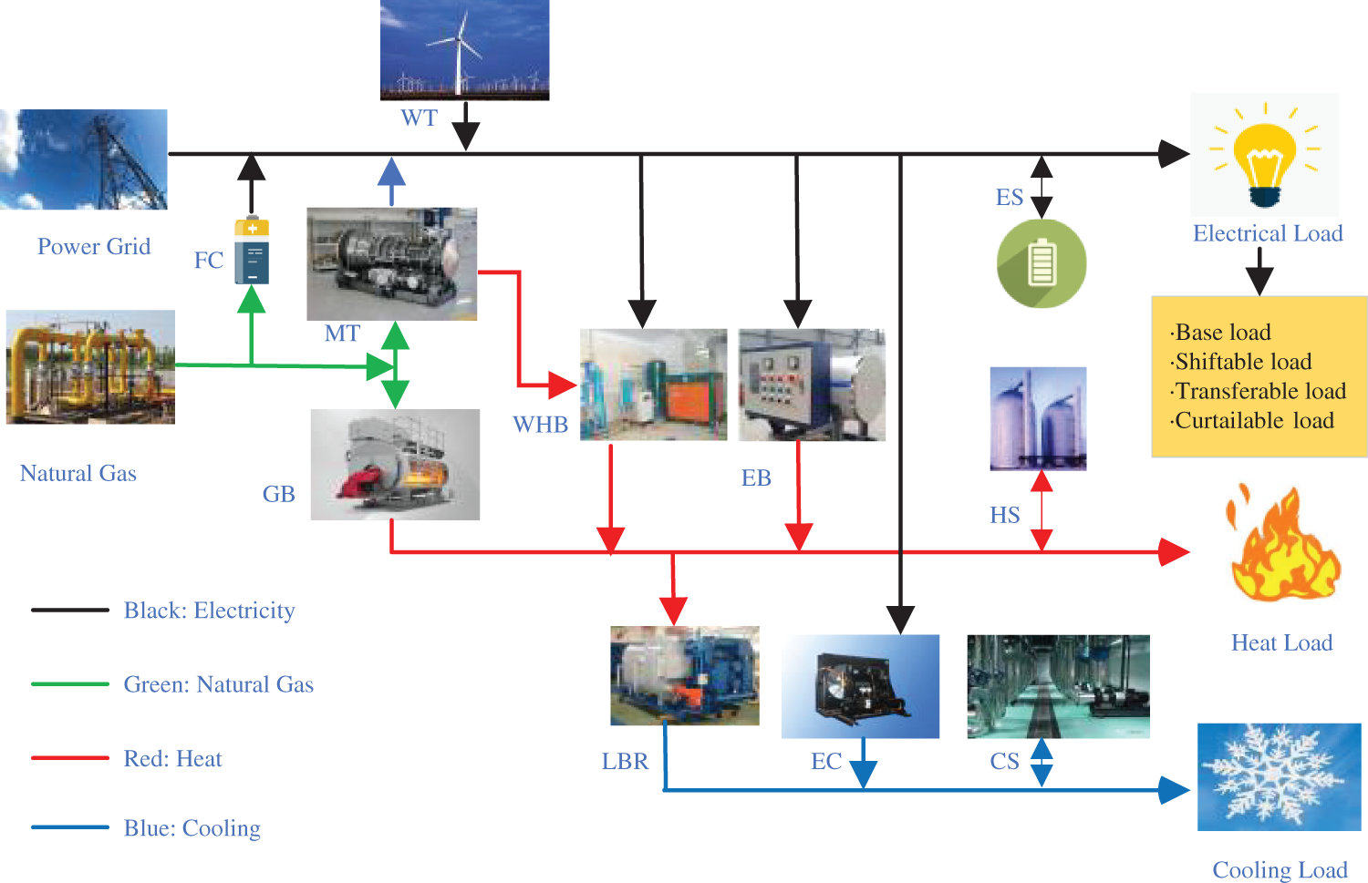
Figure 1: Structure of IES

2.1.1 Fuel Cell Model

Considering that the fuel cell (FC) is mainly responsible for electric energy dispatch in intra-day dispatch, this paper does not consider its heat energy utilization, and the power output satisfies the following constraint:

PFCmin≤PFC≤(1−ωFC)PFCmax(1)

where PFC is the output power of FC, kW; PFCminPFCmin and PFCmax are the minimum and maximum output power of FC, kW; ωFC is the backup factor, which is taken as 0.4.

The gas consumption of FC can be expressed as:

VFC=PFCηFCLNG(2)

where LNG is natural gas’s low-level heat value, which is 9.78, and ηFC is FC’s power generation efficiency, which is 0.8.

The remaining equipment models include those for MT, GB, and LBR, which are described along with operational limitations in reference [23], and EB and EC, which are described along with operational constraints in reference [24].

2.2 Controllable Load Model

The loads in community IES can be classified into the base load, shiftable load, transferable load, and curtailable load according to the energy-using characteristics.

2.2.1 Shiftable Load

The scheduling cost Fsh for shiftable load is as follows:

Fsh=∑τ=tsh−tsh+ατFcshPτsh(3)

where Lshift is the shiftable load, [t1, t2] denotes the energy usage time period of the load before the shift, [tsh−, tsh+] denotes the interval of the shift time period, and ατ=1 denotes that the load is shifted in time period t. Fcsh is the unit dispatch cost of load shifting, ¥/kWh; Pτsh is the power shifted during time period τ, kW.

2.2.2 Transferable Load

The scheduling cost Ftr of the transferable load is:

Ftr=∑τ=tr−tr+βτFctrPτtr(4)

where Ltrans is the transferable load, [t3, t4] denotes the energy usage time period of the load before the transferring, [ttr−, ttr+] denotes the interval of the transferring time period, and βτ=1 denotes that the load is transferred in time period t. Fctr is the unit dispatch cost of load transferring, ¥/kWh; Pτtr is the power transferred during time period τ, kW.

The power for each time period after the transferring shall satisfy the following constraint:

βτPmintr≤Pτtr≤βτPmaxtr(5)

where Pmintr and Pmaxtr are the minimum and maximum values of the transferred load power, respectively, kW.

To avoid frequent start-up and shutdown of power-using equipment, the minimum duration of operation for transferable loads is constrained:

∑τ=ttr−ttr−+Tmintr−1βτ≥Tmintr(βτ−βτ−1)(6)

where Tmintr is the minimum continuous operation time of the equipment, h.

2.2.3 Curtailable Load

The scheduling cost Fcut of the curtailable load is:

Fcut=Fccut∑τ=1τ=Tγτ(Pτ,1cut−Pτ,2cut)(7)

Pτcut is the power at which the load Lcut can be curtailed in the time period τ, γτ=1 is the response curtailment. where Fccut is the unit dispatch cost of load reduction, ¥/kWh; Pτ,1cut is the predicted power in the day-ahead stage in time period τ, kW; Pτ,2cut is the reduced power, kW.

Considering that frequent reductions affect users’ comfort, the upper limit of reductions and the length of reductions in a dispatch cycle should be constrained:

1) Maximum number of reduction limit:

∑t=1t=Tγτ≤Nmax(8)

where Nmax is the maximum number of the reduction.

2) Maximum and minimum reduction time:

∑τ=1τ+Tmaxcut+1(1−γτ)≥1(9)

∑τ=1τ+Tmincut−1γτ≥Tmincut(γτ−γτ−1)(10)

where Tmaxcut and Tmincut are the maximum and minimum reduction time, h, respectively.

3  Two-Stage Optimal Scheduling Model

According to the different time scales, the community IES scheduling is divided into two scheduling stages: day-ahead and intra-day stage, as shown in Fig. 2. The scheduling of the two stages is coordinated and optimized according to their different optimization objectives to ensure the economy and stability of IES operation on the basis of satisfying various constraints of IES.

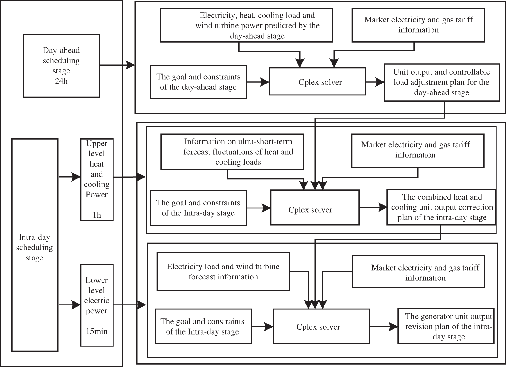
Figure 2: Two-stage optimal scheduling framework for community IES

In the day-ahead stage, the day-ahead plan values for each unit operation and controllable load adjustment are obtained based on the day-ahead short-term forecasted electric, heat, and cooling loads and wind turbine output, with the objective of minimizing the comprehensive operating cost of the community IES for one dispatching cycle and meeting the operating constraints.

In the intra-day stage, the upper-level heat and cooling energy dispatching model and the lower-level electric energy dispatching model are divided into the upper-level heat and cooling energy dispatching model and the lower-level electric energy dispatching model, based on the day-ahead dispatching plan, and the wind turbine output and the load power ultra-short-term forecast information are updated on a rolling basis, and the day-ahead plan value is revised in an incremental balancing manner to adjust the unit output. The above two stages are mixed integer linear programming problems, and Cplex solver is used to solve the output of each unit.

3.1 Wind Turbine Output Uncertainty Handling Method

In the day-ahead scheduling model, the scenario generation and reduction method are used to deal with the uncertainty of wind turbines, and historical data can be used to determine the short-term forecasted power expectation μw of wind turbines, and the power error of wind turbines is assumed to satisfy the normal distribution of N (0, σ2), then the day-ahead prediction of wind turbines is the sum of the expectation and the prediction error. A large number of original scenario sets of wind turbine power obeying probability distribution are generated by Latin Hypercube Sampling (LHS) [25], and then the above scenario sets are reduced by the simultaneous back-generation reduction method based on probability distance to derive the streamlined scenarios with corresponding probabilities, and 10 streamlined scenario sets of wind turbine power and their corresponding probabilities Pm, (m = 1,2, …,10) are obtained. Finally, the probabilities of the above scenarios and the corresponding power are multiplied and summed to obtain the power curve with the uncertainty of wind turbine output.

3.2 Day-Ahead Scheduling Optimization Model

In the day-ahead scheduling plan, both economic and environmental factors are considered to affect the operating cost of IES, and the environmental indicators are converted into economic indicators, and the minimum integrated operating cost of IES in one scheduling cycle is taken as the objective function of day-ahead scheduling, and the integrated operating cost FDH is:

minFDH=F1DH+F2DH+F3DH+F4DH(11)

where F1DH is the operating cost of the units in the system, ¥; the price of buying electricity from the grid is F2DH, ¥; the cost of dispatching controllable loads is F3DH, ¥; and F4DH is the environmental cost, ¥. In this paper, we mainly take into account the penalty cost of CO2 emissions.

F1DH=∑t=1t=T[KWTPWT(t)+Cgas(VMT(t)+VGB(t)+VFC(t))](12)

where KWT is the operating cost coefficient of the wind turbine, ¥; PWT(t) is the power output at time t, kW; Cgas is the price of natural gas per cubic meter, ¥; the amount of natural gas used by MT, GB, and FC at time t is represented by the variables VMT(t), VGB(t), and VFC(t), respectively, m3.

F2DH=∑t=1t=TKGridPGrid(t)(13)

where PGrid(t) is the amount of power purchased from the grid at time t, in kW, and KGrid is the time-of-use tariff per unit of purchased power.

F3DH=Ftr+∑n=1n=3Fnsh+Fncut(14)

where Ftr is the dispatch cost of transferable electric load, ¥; when n = 1, 2, 3 are expressed as cooling, heat, and electricity, respectively.

F4DH=∑t=1t=TKc(ζ1PGrid(t)+ζ2PMT(t)+ζ3QGB(t)+ζ4PFC(t))(15)

where Kc is the penalty factor per unit of CO2 emission, ¥; ζ1, ζ2, ζ3, and ζ4 are the CO2 emission factors per unit of power output of conventional coal-fired power plants, the CO2 emission factors per unit of power output of MT, the CO2 emission factors per unit of heat power output of GB, and the CO2 emission factors per unit of power output of FC, ¥/kg, respectively; PMT(t), QGB(t) and PFC(t) are the CO2 emission factors per unit of power output of MT, heat power output of GB, and power output of FC, respectively, at time t. The above unit CO2 emission data and penalty cost are shown in reference [26].

3.3 Constraints

The stable operation of IES in the community needs to meet certain constraints, which can be divided into equality constraints and inequality constraints.

1) The electric balance equation of each period of the system is:

{PMT(t)+PGrid(t)+PWT(t)+PFC(t)=LE(t)+PES(t)+PEB(t)+PEC(t)L(t)=Lbase(t)+Lshift(t)+Ltran(t)+Lcut(t)(16)

where PMT(t), PGrid(t) and PWT(t) are the electric power output of MT, power grid and WT, kW; PES(t) is the battery output in time period t, it is positive when stored and negative when discharged, kW; PEB(t) and PEC(t) are the electric power consumed by electric boiler and electric refrigerator in time period t, kW; LE(t), Lbase(t), Lshift(t), Ltran(t) and Lcut(t) are the total electric load, basic electric load, shiftable electric load, transferable electric load and reducible electric load of time period t, kW.

2) Heat load supply and demand balance:

{QMT(t)=QMT1(t)+QMT2(t)QGB(t)=QGB1(t)+QGB2(t)PEB(t)=PEB1(t)+PEB2(t)(17)

where QMT(t) and QGB(t) denote the combined heat output of MT and GB, respectively, kW; the power supplied by MT, GB, and EB to the heat load is denoted by QMT1(t), QGB1(t) and PEB1(t), kW; the power supplied by MT, GB, and EB to the LBR absorption refrigeration is denoted by QMT2(t), QGB2(t) and PEB2(t), respectively.

{QMT1(t)+QGB1(t)+ηEBPEB1(t)=Q(t)+QHS(t)Q(t)=Qbase(t)+Qshift(t)+Qcut(t)(18)

where ηEB is the energy-efficiency ratio of EB heat production, and is taken as 3; QHS(t) is the power of the heat storage tank, which is positive when heat is stored and negative when heat is released, and is kW; Q(t), Qbase(t), Qshift(t) and Qcut(t) are the total, basic, transferable, and curtailing heat loads in time t, respectively, kW.

3) Cooling load supply and demand balance:

{Rα(t)+ηECPEC(t)=C(t)+CCS(t)C(t)=Cbase(t)+Cshift(t)+Ccut(t)(19)

where Rα(t) denotes the LBR’s cooling capacity in kW; ηEC stands for energy efficiency of EC cooling, taken as 4; the power of a storage tank is CCS(t), positive for storage and negative for discharge, kW; the overall cooling load, base cooling load, shiftable cooling load, and curtailable cooling load, all expressed in kW, are designated as C(t), Cbase(t), Cshift(t) and Ccut(t), respectively.

In actual operation, MT units are subject to the following climbing constraints:

PMTdown≤PMT(t)−PMT(t−1)≤PMTup(20)

where PMTdown and PMTup are the maximum downward and upward climbing rate of the equipment, in the text are taken as 80 kW/h.

3.4 Intra-Day Rolling Optimization Model

The day-ahead plan determines the operation state of the shiftable load, transferable load, and curtailable load in the intra-day plan, and no optimization is necessary. Given the frequent power fluctuations in the intra-day operation plan, as well as the energy storage equipment’s service life and the fact that it has reached the maximum number of energy storage and discharge in the day-ahead plan, participation of energy storage equipment in the intra-day dispatch plan is not considered for the time being.

The upper-level scheduling model is used to smooth out cooling and heat power fluctuations with a slower response rate, with a scheduling time domain of 2 h and a control time domain of 1 h. The lower-level scheduling model is used to smooth out electrical power fluctuations with a faster response rate, with a scheduling time domain of 1 h and a control time domain of 15 min.

The intra-day scheduling strategy is shown in Fig. 3, with 15 min as a time period and a total of 96 time periods in a scheduling cycle. At time k, the power of the heat and cooling loads is predicted in the [k + 4, k + 12] time period, and the planned values of the heat and cooling equipment output in the [k + 4, k + 8] time period are adjusted according to the predicted power. Similarly, at the moment k + 4, the heat and cooling power in the time period [k + 8, k + 16] is predicted and the equipment output plan of [k + 8, k + 12] is adjusted, and so on rolling backward for optimization. Correspondingly, at moment k, the system forecasts the power of the electrical load during the time period [k + 1, k + 5], adjusts the equipment output data for the time period [k + 1, k + 2] according to the forecasted power and rolls backward for optimization. Because of the difference in the rolling cycles of heat and cooling energy and electrical energy, the scheduling of heat and cooling energy always takes priority over electrical energy scheduling at the same time point, thus enabling the scheduling of heat and cooling energy and electrical energy to be performed separately.

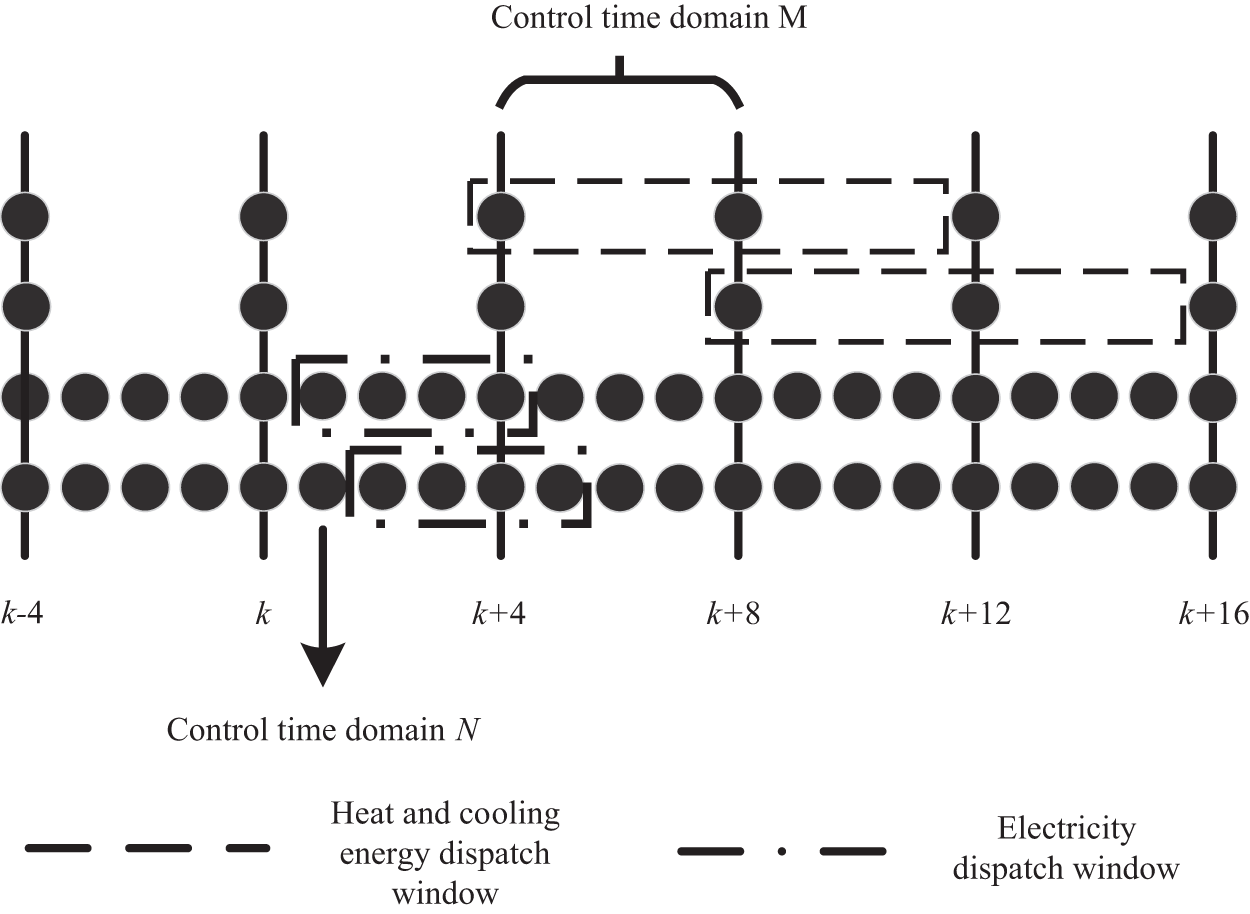
Figure 3: Dispatch of cooling, heat and electricity power at different time scales

3.4.1 Upper-Level Rolling Optimization Smoothing Model

1) The upper-level rolling optimization objective function

In the upper-level scheduling strategy, the output capacity of each equipment is adjusted according to the fluctuation of hot and cooling loads, and its objective function is:

ΔFQCRT=min∑t=kk+2M(ΔFMT(t)+ΔFGB(t)+ΔFEB(t)+ΔFEC(t))(21)

where ΔFQCRT is the total dispatch cost of smoothing the heat and cooling loads, ¥; ΔFMT(t) and ΔFGB(t) are the gas costs consumed by MT and GB, ¥; ΔFEB(t) and ΔFEC(t) are the electricity costs consumed by EB and EC, ¥; M is the control time domain of heat and cooling energy dispatch, h.

2) Upper-level optimization constraints

(1) Heat energy balance constraint

ΔQMT(t)+ΔQGB(t)+ΔQEB(t)=ΔQ(t)(22)

where ΔQMT(t), ΔQGB(t) and ΔQEB(t) are the heat production power adjustment amounts of MT, GB, and EB, respectively, with increment as positive and downgrade as negative, kW; ΔQ(t) is the error between heat load and the predicted value of the day-ahead stage, kW.

(2) Cooling energy balance constraint

ΔCEC(t)+ΔRa(t)=ΔC(t)(23)

where ΔCEC(t) and ΔRa(t) are the cooling power adjustments of EC and LBR, respectively, with positive for incremental development and negative for downward adjustment, kW; ΔC(t) is the error between the cooling load at time t and the predicted value at the previous day stage, kW.

(3) Unit constraints

{−0.1QMTmax≤ΔQMT(t)≤0.1QMTmax−0.2QEBmax≤ΔQEB(t)≤0.2QEBmax−0.1QGBmax≤ΔQGB(t)≤0.1QGBmax−0.2CECmax≤ΔCEC(t)≤0.2CECmax−0.1Ramax≤ΔRa(t)≤0.1Ramax(24)

3.4.2 Lower-Level Rolling Optimization Smoothing Model

1) Lower-level rolling optimization objective function

In the lower-level dispatching strategy, the output of the power supply equipment is adjusted according to the fluctuation of the electric load and in conjunction with the adjusted output plan of the upper-level combined heat and cooling supply equipment, with the minimum system dispatching cost as the objective function:

ΔFERT=min∑t=kk+4N(ΔFGrid(t)+ΔFFC(t))(25)

where ΔFGrid(t) and ΔFFC(t) are the grid power purchase and FC fuel costs, respectively, ¥; N is the control time domain of power dispatch, h.

2) Constraints on lower-level optimization

(1) Constraint on electrical power balance:

ΔPGrid(t)+ΔPFC(t)=ΔPE(t)+ΔPEB(t)+ΔPEC(t)(26)

where ΔPGrid(t), ΔPFC(t) and ΔPE(t) are the electric power adjustment of the grid, FC, and the error of the electric load, respectively, kW; the amount of electricity used by EB and EC, respectively, is denoted by ΔPEB(t) and ΔPEC(t), and the increase is positive and the decrease is negative, kW.

(2) The power fluctuations in the intra-day stage should be kept to the contact line with the grid in order to preserve the stability of the external grid:

−0.02PGridmax≤ΔPGrid(t)≤0.02PGridmax(27)

(3) FC constraint

−ωFCPFCmax≤ΔPFC(t)≤ωFCPFCmax(28)

4  Example Analysis

4.1 Basic Data

In this paper, a typical summer day in a community is selected for the calculation. The energy structure of the community is shown in Fig. 2. The standard deviation of the wind turbine power prediction error σ = 0.2 μw, the natural gas price is 2.5 ¥/m3, the rated capacity of the energy storage equipment is 300 kWh. The parameters for controllable load scheduling are shown in Appendix Table A1 and the output parameters for the device are shown in Appendix Table A2. The wind power output as well as the electrical, thermal, and cooling loads are shown in Appendix Figs. A1–A4. Based on the historical electricity price data of the area, the following time-sharing tariff is developed, with the same price for electricity purchase and sale, 0.25 ¥/kWh for the valley hours from 0:00 to 7:00, and 0.82 ¥/kWh for the peak hours from 10:00 to 15:00 and 18:00 to 21:00. The tariff is 0.82 ¥/kWh for peak hours from 10:00 to 15:00 and 18:00 to 21:00, and 0.53 ¥/kWh for weekdays from 7:00 to 10:00, 15:00 to 18:00 and 21:00 to 24:00.

In order to verify the advantages of two-stage rolling optimal scheduling considering controllable loads of heat, cooling and electricity, the following cases are set up for comparison:

Case 1: Comprehensive demand response is not considered, and only day-ahead optimal scheduling is performed.

Case 2: Comprehensive demand response is considered and only day-ahead optimization is performed.

Case 3: Comprehensive demand response is considered, and two-stage rolling optimization scheduling is carried out.

All the above 3 cases have the same conditions except for different optimization scheduling methods. The computer processor used in this paper is Intel(R) Core (TM) i5-8300H CPU and the simulation software used is MATLAB version 2018b. The simulation time for the case 3 is 63.08 s.

4.2 Day-Ahead Optimal Scheduling Analysis

1) Comprehensive cost analysis:

The combined operating costs of the system under case 1 and case 2 are shown in Table 1. Fig. 4 shows the electrical power balance for case 2, Fig. 5 shows the heating power balance for case 2, and Fig. 6 shows the cooling power balance for case 2.

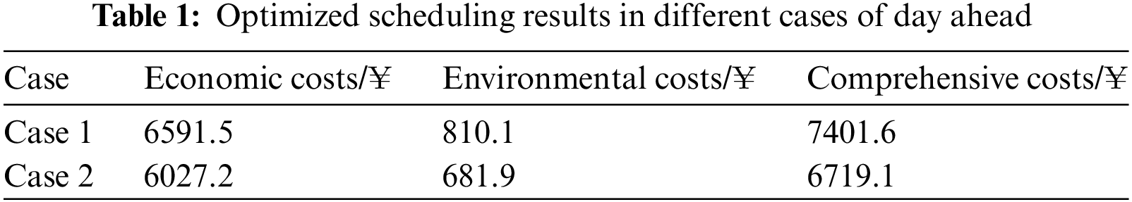
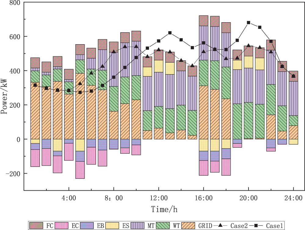
Figure 4: Balanced of power load (case 2)

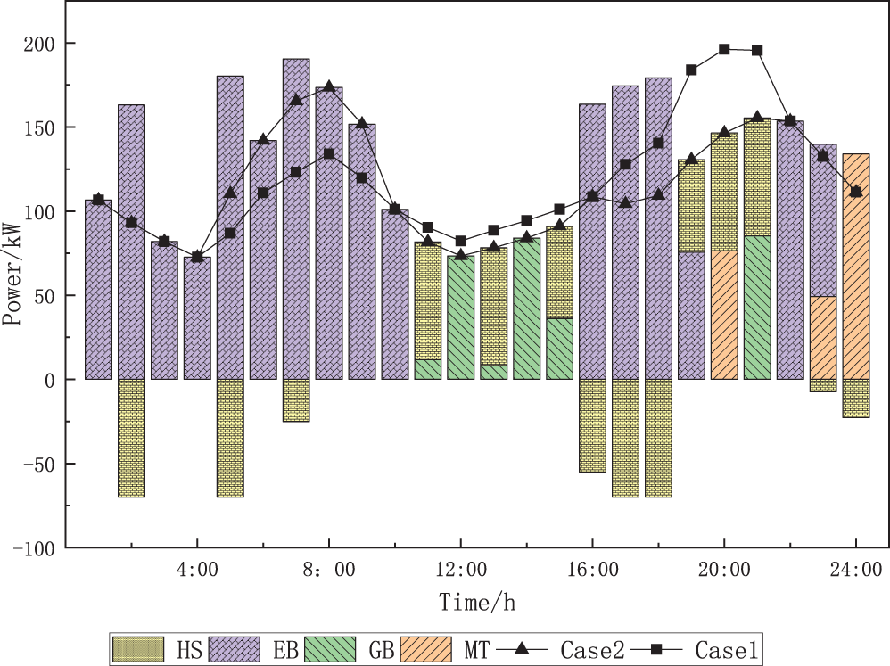
Figure 5: Balanced of heating load (case 2)

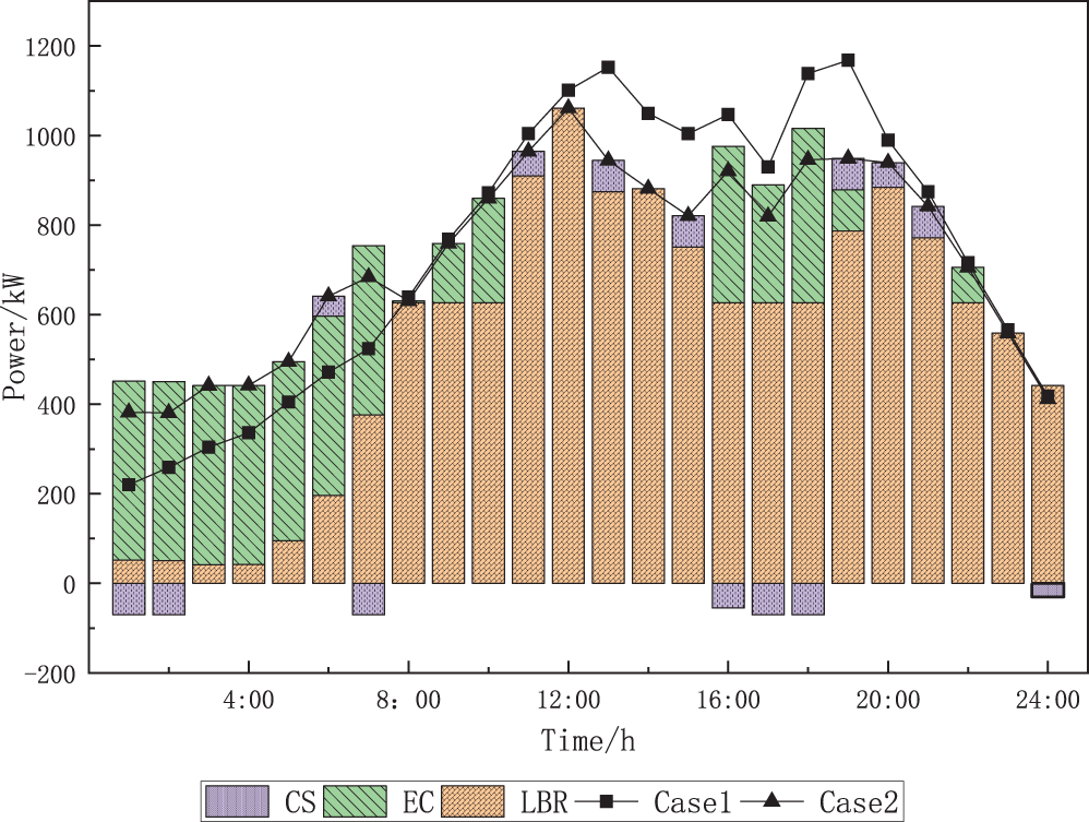
Figure 6: Balanced of cooling load (case 2)

As can be seen from Table 1, after optimizing the scheduling of demand-side controllable loads, the cost of the system is reduced in both economic and environmental terms, and its combined operating cost after considering demand response is 9.2% lower than when it is not considered. Figs. 4–6 show that during the valley hours of 00:00–08:00 tariff, the electric, heat, and cooling loads are in the valley hours, and the grid primarily supplies the electric load, EB primarily supplies the heat load, and EC primarily supplies the cooling load, and some energy is stored in the energy storage equipment by taking full advantage of the lower tariff. During 11:00–16:00 is the first peak hour of electricity price, as the electric and cooling loads gradually rise, the power output of MT continues to increase and reach full load state operation. From an economic standpoint and because there are currently plenty of wind power resources available, the electric load is primarily supplied by the MT, WT, and battery. The cooling load is provided by absorbing the waste heat from the MT and the heat supplied by the GB for LBR cooling. During 19:00–22:00, the second peak hour of the tariff, the working condition of each unit of the system is basically the same as 11:00–16:00. During 08:00–11:00 and 16:00–19:00 and 22:00–24:00, the electric heating and cooling load has not yet reached its peak and the tariff is in the normal period. As a result, the system boosts the output of EB, EC, and other electric heating and cooling conversion devices in order to lower GB’s fuel consumption and CO2 emissions and hence lower fuel costs. In particular, the power output of FC has been maintained at the maximum power allowed during the day-ahead period because of the reserve capacity and the low cost of power generation.

2) Controllable load analysis before and after demand response:

From the load curves before and after demand response in Figs. 4 and 6, it can be seen that by adjusting part of the controllable load to the valley hours, the pressure of concentrating the units in a few hours due to over-concentration of load is relieved, and the peak-valley difference of load is effectively reduced. Specifically, the peak value of electric load was reduced from 680 to 545 kW before demand response, and the valley value was increased from 273 to 284 kW; the peak value of heat load was reduced from 196 to 174 kW before demand response, and the valley value remained unchanged at 73 kW; the peak value of cooling load was reduced from 1168 to 1061 kW before demand response, and the valley value was increased from 220 to 381 kW.

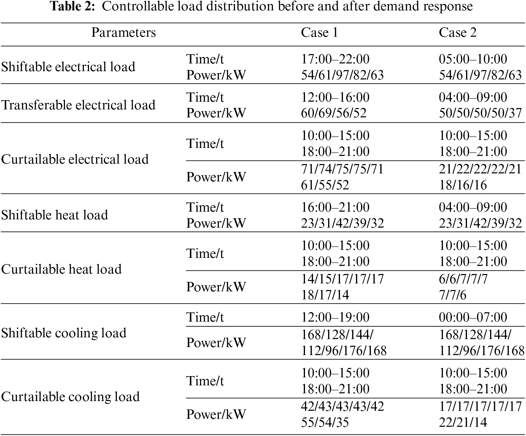
The distribution of the controllable load prior to and during the demand response is shown in Table 2. The duration of the load and the power in each period are changed before and after the shiftable load responds, and the shiftable electric, heat, and cooling loads are moved to load valley hours. The cuttable load is reduced during the peak hours of 10:00–15:00, 18:00–21:00, etc., but there are not any extended or frequent cuts because the maximum number of cuts and the duration of cuts are limited. The overall amount of energy consumed does not vary, but the transferred load is different from the period and power before the demand response.

4.3 Intra-Day Optimal Scheduling Analysis

The intra-day optimal dispatch is case 3, and the optimization results are shown in Fig. 7. Its day-ahead and intra-day stages are scheduled for heat and cooling energy on the hourly time scale, while the intra-day electric energy is scheduled on the minute time scale.

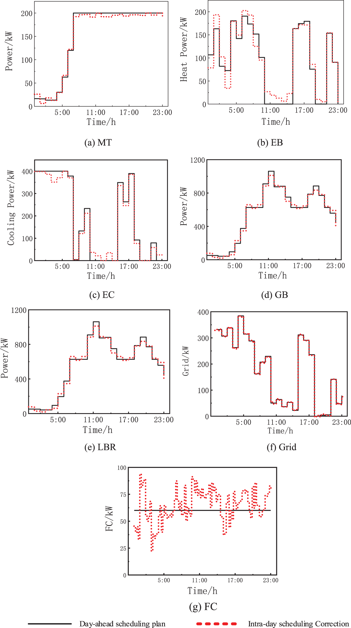
Figure 7: Optimization results in different time scales

From Figs. 7a–7e, it can be seen that for the upper-level heat and cooling energy dispatch: In the periods of 01:00–03:00, 05:00–08:00, 14:00–20:00, the heat power fluctuation is mainly maintained by EB and GB incremental generation to keep the heat power balance because the heat load ultra-short-term forecast value is larger than the day-ahead forecast value, and in the periods of 0:00–01:00, 03:00–05:00, 14:00–20:00. In the periods of 0:00–01:00, 03:00–05:00, 08:00–12:00, 20:00–0:00, the ultra-short-term forecast of heat power is smaller than the previous forecast, but the cooling load is larger than the previous forecast in some of the above periods, so EB and GB still increase the heat power to supply LBR absorption cooling, while MT reduces the output power to smooth out the heat load fluctuation. LBR and EC correct the output power to maintain the balance of cooling power in order to maintain the cooling load, and since LBR relies on absorption heat power for cooling, when the sum of EB, MT, and GB output heat power is greater than zero, from the viewpoint of the system economy, LBR cooling is given priority to provide the required cooling load, and the shortage is supplemented by EC cooling.

From Figs. 7f–7g, it can be seen that for lower-level electric power dispatch, the difference in forecast time scales between day-ahead and intra-day dispatch leads to large fluctuations in unit output, and the basic by FC during the intra-day stage smooths out the variations in electric power in order to guarantee the stability of the external grid, and the grid contact line power is maintained as much as possible on the day-ahead schedule.

5  Conclusion

In this paper, a two-stage optimal dispatch model of community IES with controllable loads is proposed for community IES, considering the differences in response rates of various controllable loads and hot and cooling electricity on different time scales. The inferences that can be made are as follows:

1) The participation of controllable loads of cooling, heat, and electricity in optimal scheduling can effectively reduce the comprehensive operating costs of community IES.

2) The intra-day two-stage rolling optimization model is capable of dispatching heat, cooling energy, and electric energy at different time scales, respectively, enabling the system to timely and effectively smooth out the prediction errors on both sides of the source and load, and realize the stable operation of community IES and connected large grids.

In this paper, we have considered the impact of load demand response on the optimal scheduling of the system, but the implementation of demand side management will change the way of using energy, resulting in customer dissatisfaction. Therefore, not only economic issues but also customers’ satisfaction needs to be considered in future work studies.

Acknowledgement: None.

Funding Statement: This work was supported in part by the National Natural Science Foundation of China (51977127), Shanghai Municipal Science and Technology Commission (19020500800), and “Shuguang Program” (20SG52) Shanghai Education Development Foundation and Shanghai Municipal Education Commission.

Author Contributions: The authors confirm contribution to the paper as follows: study conception ancdesign: Ming Li; data collection: Rifucairen Fu; analysis and interpretation of results: Tuerhong Yaxiaer; draft manuscript preparation: Yunping Zheng. All authors reviewed the results and approved the final version of the manuscript.

Availability of Data and Materials: Data supporting this study are included within the article.

Conflicts of Interest: The authors declare that they have no conflicts of interest to report regarding the present study.

References

1. Chen, Z., Wen, B., Zhu, Z. (2023). Multi time scale optimal scheduling of regional comprehensive energy systems considering wind power correlation. Power Automation Equipment, 43(8), 25–32. [Google Scholar]

2. Huang, W., Zuo, X., Liu, Y. (2021). A comprehensive energy system scheduling architecture based on multiple blockchain structures. Power System Automation, 45(23), 12–20. [Google Scholar]

3. Wang, K., Zhang, Y., Ji, X., Shi, J., Liu, J. et al. (2022). Comprehensive energy system planning taking into account flexible electric loads. Journal of Anhui University (Natural Science Edition), 46(6), 67–75. [Google Scholar]

4. Lei, X., Ma, P., Song, Z., Li, W. (2022). A flexible intraday load dispatch model taking into account wind power forecast error. Power Generation Technology, 43(3), 485–491. [Google Scholar]

5. Wang, L., Du, Z., An, X., Zhao, W. (2021). Multi-objective optimal scheduling of regional integrated energy system taking into account ORC and flexible load. Modern Electronic Technology, 44(19), 129–135. [Google Scholar]

6. Deng, J., Jiang, F., Wang, W., He, J., Zhang, X. et al. (2022). Low-carbon operation of an integrated energy system considering electric-thermal flexible load and hydrogen energy refined modeling. Grid Technology, 46(5), 1692–1704. [Google Scholar]

7. Ma, Y., Xie, J., Zhao, S., Wang, Z., Luo, Z. (2022). Multi-objective optimal scheduling of active distribution networks considering integrated energy system access in parks. Power System Automation, 46(13), 53–61. [Google Scholar]

8. Lin, Z., Jiang, C., Chen, M., Shang, H., Zhao, H. et al. (2020). Low-carbon economic operation of integrated energy system taking into account flexible load. Electric Power Construction, 41(5), 9–18. [Google Scholar]

9. Cui, P., Shi, J., Wen, F., Sun, L., Dong, C. et al. (2017). Optimal allocation of energy hubs accounting for integrated demand side response. Power Automation Equipment, 37(6), 101–109. [Google Scholar]

10. He, Z., Xu, C., Liu, Y., Hua, H., Dong, S. (2017). A comprehensive demand side response model for factories considering multi energy collaboration. Power Automation Equipment, 37(6), 69–74. [Google Scholar]

11. Fu, Y., Jiang, Y., Li, Z., Wei, C. (2014). Economic optimization of microgrid scheduling taking into account shiftable loads. Journal of China Electrical and Mechanical Engineering, 34(16), 2612–2620. [Google Scholar]

12. Zou, Y., Zeng, A., Hao, S., Ning, J., Ni, L. (2023). Multi-time scale optimal scheduling of integrated energy system under stepped carbon trading mechanism. Grid Technology, 47(6), 2185–2198. [Google Scholar]

13. Liu, G., Han, D., Liu, C., Guo, H., Fan, R. et al. (2023). Dual time-scale optimal scheduling of integrated energy system considering dual demand response and stepped carbon trading. Power Automation Equipment, 43(5), 218–225. [Google Scholar]

14. Yang, M., Hu, Y., Qian, H., Liu, F., Wang, X. et al. (2023). Day-ahead and intraday multi-timescale optimal scheduling of integrated energy distribution networks accounting for carbon emissions. Power System Protection and Control, 51(5), 96–106. [Google Scholar]

15. Xu, J., Ma, G., Gao, C., Shen, J., Yan, Z. et al. (2022). Day-ahead-intraday optimal scheduling of integrated energy systems based on wind-scenario generation. Distributed Energy, 7(4), 18–27. [Google Scholar]

16. Ma, Z., Jia, Y., Han, X., Kang, L., Ren, H. (2022). Two-tier optimal scheduling of integrated energy systems considering dynamic time intervals. Grid Technology, 46(5), 1721–1730. [Google Scholar]

17. Zhang, L., Dai, W., Zhao, B., Zhang, X., Liu, M. et al. (2023). Multi-time-scale economic scheduling method for electro-hydrogen integrated energy system based on day-ahead long-time-scale and intra-day MPC hierarchical rolling optimization. Frontiers in Energy Research, 11, 1132005. [Google Scholar]

18. Wang, Z., Tao, H., Cai, W., Zhang, L., Meng, J. (2023). Optimal scheduling study of multi-timescale rolling optimization in combined cooling, heating and power system. Journal of Solar Energy, 44(2), 298–308. [Google Scholar]

19. Zhao, W., Chen, Z., Wu, S., Yu, T. (2022). Multi-timescale optimal scheduling of micro-energy networks containing solar thermal. Heilongjiang Power, 44(2), 119–126. [Google Scholar]

20. Wang, Z., Tao, H., Zhang, L. (2022). Research on rolling optimization operation method for combined cooling, heating and power supply system with multiple time scales. Journal of Power Engineering, 42(3), 276–285. [Google Scholar]

21. Xu, L., Yi, Y., Zhu, C., Zhao, B., Xiang, Z. et al. (2014). Optimal energy scheduling of microgrid with multiple time scales considering wind power stochasticity. Power System Protection and Control, 42(23), 1–8. [Google Scholar]

22. Qiu, Z., Wang, B., Ben, S., Hu, N. (2019). A two-tier optimal allocation planning model for regional integrated energy system accounting for uncertainty. Power Automation Equipment, 39(8), 176–185. [Google Scholar]

23. Liu, R., Ma, T., Sun, G. (2023). Optimized scheduling of community integrated energy systems accounting for integrated demand response. Electrical Drives, 53(1), 66–73. [Google Scholar]

24. Liu, R., Ma, T., Gao, Y., Liang, Y., Zhu, Y. et al. (2020). Low-carbon economic dispatch of community integrated energy system considering demand-side cooperative response. Journal of Shanghai Electric Power University, 36(5), 421–430. [Google Scholar]

25. Wang, Z., Fang, Z., Liu, W., Wang, L., Wang, C. et al. (2019). Probabilistic multi-scenario based robust operation optimization for flexible distribution networks. Power Automation Equipment, 39(7), 37–44. [Google Scholar]

26. Wu, Y., Ma, X., Sun, Y., Fang, H. (2012). Evaluation and analysis of comprehensive economic benefits after high penetration rate access of microgrid. Power System Protection and Control, 40(13), 49–54. [Google Scholar]

Appendix

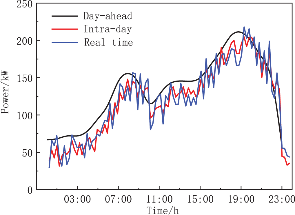
Figure A1: Output of WT

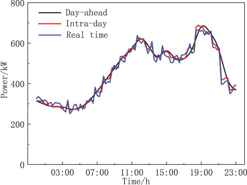
Figure A2: Power load

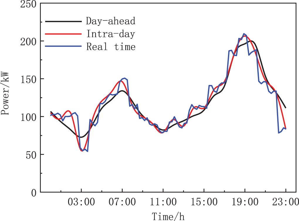
Figure A3: Heat load

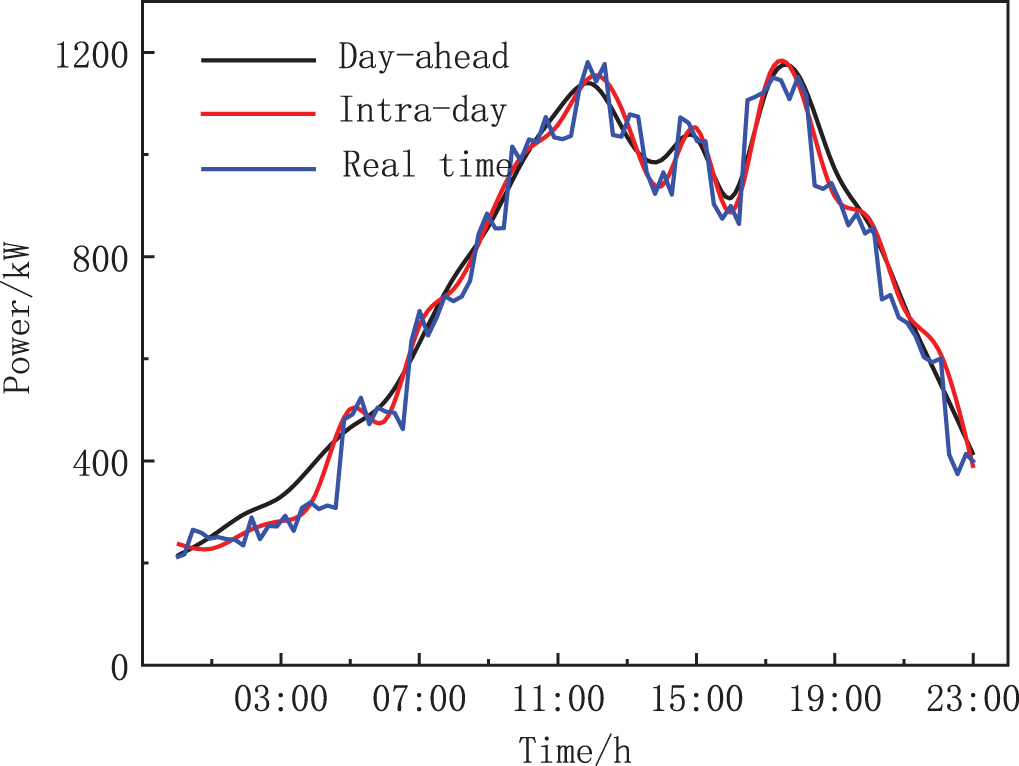
Figure A4: Cooling load