Prediction on Failure Pressure of Pipeline Containing Corrosion Defects Based on ISSA-BPNN Model

Nomenclature

1  Introduction

As the fifth largest transportation mode after highway, railway, water, and air transportation, pipeline transportation plays an important role in oil and natural gas transportation because of its advantages such as large transportation capacity, economy and environmental protection, low energy consumption, and not easy to be restricted by external conditions [1]. By 2022, the mileage of newly built oil and gas pipelines in China is about 4,668 kilometers, and the total mileage of oil and gas pipelines has reached 155,000 kilometers [2]. Pipeline failure will cause huge losses to enterprises and society, and corrosion is one of the main reasons for pipeline failure [3–5]. Therefore, it is of great significance to study the failure pressure of corrosion defect pipelines to ensure the pipeline’s safe operation.

Scholars at home and abroad have studied the failure pressure prediction model of oil and gas pipelines, for example, the AGA Pipeline Research Committee proposed NG-18 circumferential failure stress calculation formula based on fracture mechanics, Kiefner and others proposed B31G criterion for residual strength calculation of single corrosion defect, and ASME revised it several times later, the most commonly used version is ASME B31G-2009 [6]. It also has the LPC criterion by British Gas, the PCORRC criterion by Battelle, and the DNV-RP-F101 standard by British Gas and the Norwegian classification society DNV [7–9]. However, the above-mentioned traditional forecasting models are conservative and have low accuracy, which has certain limitations. Some Chinese scholars use the ANSYS finite element analysis method to establish prediction models for pipelines with different corrosion degrees to predict pipeline failure pressure [10,11]. This method can build prediction models according to the actual characteristics of pipelines and failure criteria in different environments, but the calculation process is complicated and is not conducive to prediction.

In recent years, with the development of computer and intelligent algorithms, the research of pipeline failure pressure prediction models has been more inclined to computer-intelligent algorithms. Liu et al. [12] predicted the residual strength of a defective pipeline based on the Support Vector Machine (SVM) algorithm. Jiang et al. [13] established a hybrid prediction model based on support vector regression (SVR) and Particle Swarm Optimization (PSO). Some scholars predicted the residual strength of defective pipelines based on the Extreme Learning Machine (ELM) algorithm [14]. Most scholars established the prediction model of pipeline failure pressure based on the BP neural network [15,16].

To sum up, only a few scholars based on the ELM algorithm of pipeline failure pressure prediction model, the accuracy of the ELM model is about 11%. Most scholars have established pipeline failure pressure prediction models based on the BP neural network, the accuracy of the BPNN model is about 10%. Li et al. [17] used ABAQUS and MATLAB to analyze the failure pressure of pipelines with axial double corrosion defects in cold areas, proving the BPNN model is accurate in predicting failure pressure. This paper also establishes a prediction model of pipeline failure pressure based on the BP neural network. Because the BP neural network adopts error backpropagation training, it needs many iterations to get the optimal model parameters, and the convergence rate is usually slow. Therefore, this paper introduces a Logistic chaotic map to propose an ISSA algorithm, to further improve the accuracy and stability of the BP neural network model prediction, and provide technical support for failure pressure prediction and safety management of corroded pipelines.

2  BPNN and Optimization Algorithm

2.1 BPNN Model

BPNN is a multi-layer feedforward network, which consists of an input layer, a hidden layer, and an output layer, the network structure diagram is shown in Fig. 1 [18]. The learning process of BP neural network includes two stages: forward propagation of signal and back propagation of error. In the first stage, the network input signal is transferred from the input layer to the hidden layer, and then transferred to the output layer after the activation operation of the hidden layer activation function. After the hidden layer activation function, the output of the hidden layer can be controlled in the range of 0~1, and then transferred to the output layer. In the second stage, the network carries out back propagation according to the error comparison between the predicted value and the experimental value. By adjusting the weights and thresholds between neurons, the whole network can be corrected continuously in the direction of error reduction.

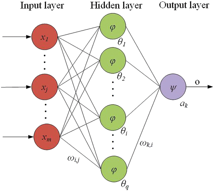
Figure 1: BP neural network structure diagram

2.2 SSA Optimization Algorithm and Its Improvement

2.2.1 SSA Optimization Algorithm

In 2020, Xue et al. [19] proposed SSA inspired by sparrows’ foraging behavior and anti-predation behavior. The algorithm divides all individuals of a sparrow population into two roles: discoverer and participant. Among them, the discoverer has a higher energy reserve and is responsible for finding foraging places with more food. The participants had lower energy reserves, but they were always able to find the finder who provided the best food source and then came close to competing for food. The energy reserve of the sparrow individual is represented by Fitness Value in the actual modeling process. In the whole sparrow population, some sparrows are always aware of the appearance of predators. This part of the sparrow accounts for 10% to 20% of the total population, and this part of the sparrow is called the guard. Discoverers and participants can change roles with each other, but it is necessary to ensure that the proportion of discoverers and participants in the whole population remains unchanged.

In the process of solving the actual d-dimensional problem to be optimized by SSA, the population composed of n sparrows is set as:

X=(x1,1…x1,d⋮⋱⋮xn,1⋯xn,d)(1)

The fitness value of the whole sparrow population can be expressed as:

FX=[f([x1,1⋯x1,d])⋮f([xn,1⋯xn,d])](2)

where: f represents the fitness value of a single sparrow in the population.

In the actual search process, according to the rules, the update of the finder position in the population is described by the following Eq. (3):

Xi,jt+1={Xi,jt⋅exp⁡(−iα⋅itermax)ifR2<STXi,jt+Q⋅LifR2≥ST(3)

where: t represents the current iteration algebra, j = 1, 2, 3, …, d. Xi,j represents the position information of the i-th sparrow in the j-th dimension. α is a random number between (0, 1). itermax represents the maximum number of iterations. R2(R2∈[0,1]) indicates the warning value, ST(ST∈[0.5,1]) denotes safe values. Q is a random number and obeys normal distribution. L is a matrix with dimensions 1 × d, where each element is 1.

According to the predator rule, the update of the participant position is described by the following Eq. (4):

Xi,jt+1={Q⋅exp⁡(Xworst−Xi,jti2)ifi>n/2Xpt+1+|Xi,jt−Xpt+1|⋅A+⋅L otherwise (4)

where: Xp represents the ideal food source position found by the current discoverer, and Xworst denotes the current overall worst position. The entries of matrix A, which has dimensions of 1 × d, are randomly assigned to either 1 or −1, and satisfies A+=AT(AAT)−1.

The initial position of the guard is randomly generated in the population, and the update of its position is described by the following Eq. (5):

Xi,jt+1={Xbestt+β⋅|Xi,jt−Xbestt|iffi>fgXi,jt+K⋅(|Xi,jt−Xworstt|(fi−fw)+ε)iffi=fg(5)

where: Xbest is the best food source location at present. K and β are step size control parameters, and β is a random number with the normal distribution of mean value 0 and variance 1; K is a random number over [1,1] and also indicates the direction in which the sparrow moves. fi, fg and fw are the current individual, global best, and worst fitness values, respectively. ε is the minimum constant set to avoid zero denominators.

2.2.2 ISSA Optimization Algorithm by Logistic Chaotic Map

A common example of a chaotic map is the logistic chaotic map. It is extensively utilized because of its straightforward mathematical form [20]. In this paper, based on a Logistic chaotic map, an improved sparrow algorithm is proposed, which optimizes the initial population. Its mathematical expression is:

Yn+1=aYn(1−Yn)(6)

where: Yn∈[0,1], a∈[0,4] is the Logistic parameter.

The closer a is to 4, the more the range of Y is evenly distributed to the whole [0,1] region. When a is 4, the system is in a completely chaotic state, and the uniformity of mapping distribution reaches the extreme value, so the value of a is 4 in this paper.

3  Modeling and Evaluation

3.1 Model Building

When improving the SSA Optimization Algorithm, the Logistic chaotic map strategy is mainly used to initialize the population. The flow of ISSA-BP prediction model is shown in Fig. 2.

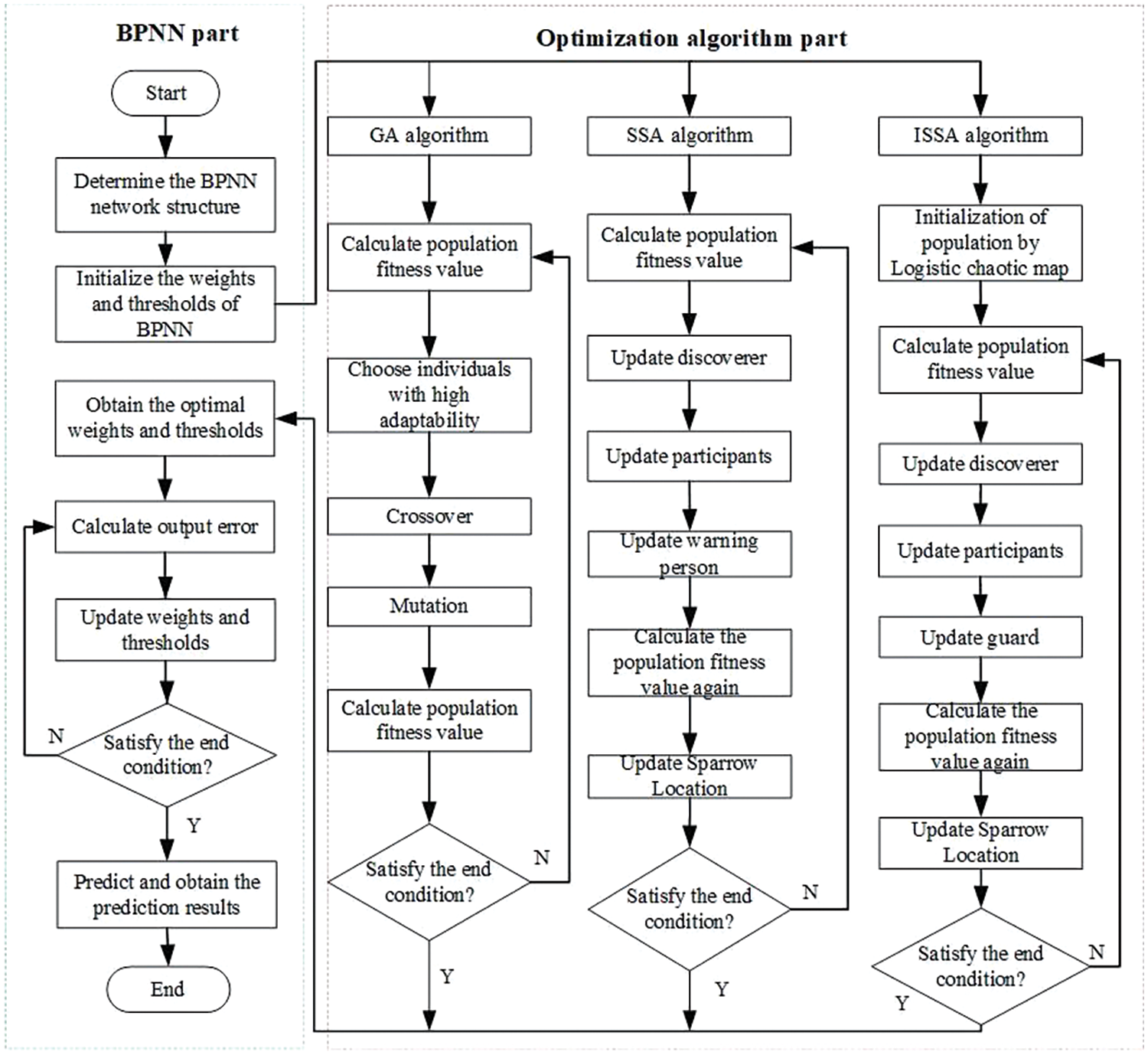
Figure 2: Flowchart of the optimized mode

(1) Using a Logistic mapping strategy to initialize population, and iteration times and initialize the proportion of discoverer and participant.

(2) Calculate and arrange fitness values.

(3) Update the discoverer’s location.

(4) Update the participant’s location.

(5) Update the guard’s location.

(6) Calculate the fitness value and update the sparrow position.

(7) If the termination condition is satisfied, end and output the result; otherwise, repeat steps 2–6.

3.2 Evaluation Indicators

To evaluate the prediction effect, mean absolute error (MAE), root mean square error (RMSE), mean absolute percentage error (MAPE), and determination coefficient R2 were selected as evaluation indexes. The smaller the values of MAE, RMSE, and MAPE, and the larger the values of R2, the higher the prediction accuracy of the model. It is described by the following Eqs. (7)–(10):

MAE=1N∑i=1N|PF−PF∧|(7)

RMSE=1N∑i=1N(PF−PF∧)2(8)

MAPE=1N∑i=1N|PF−PF∧PF|×100% (9)

R2=1−∑i=1n⁡(PF−PF∧)2∑i=1n⁡(PF−PF−)2(10)

where: PF is the experimental value of pipeline failure pressure; PF∧ is the predicted value of pipeline failure pressure; PF− is the average value of the experimental value of pipeline failure pressure; N is the total number of test samples.

4  Example Analysis

4.1 Data Acquisition

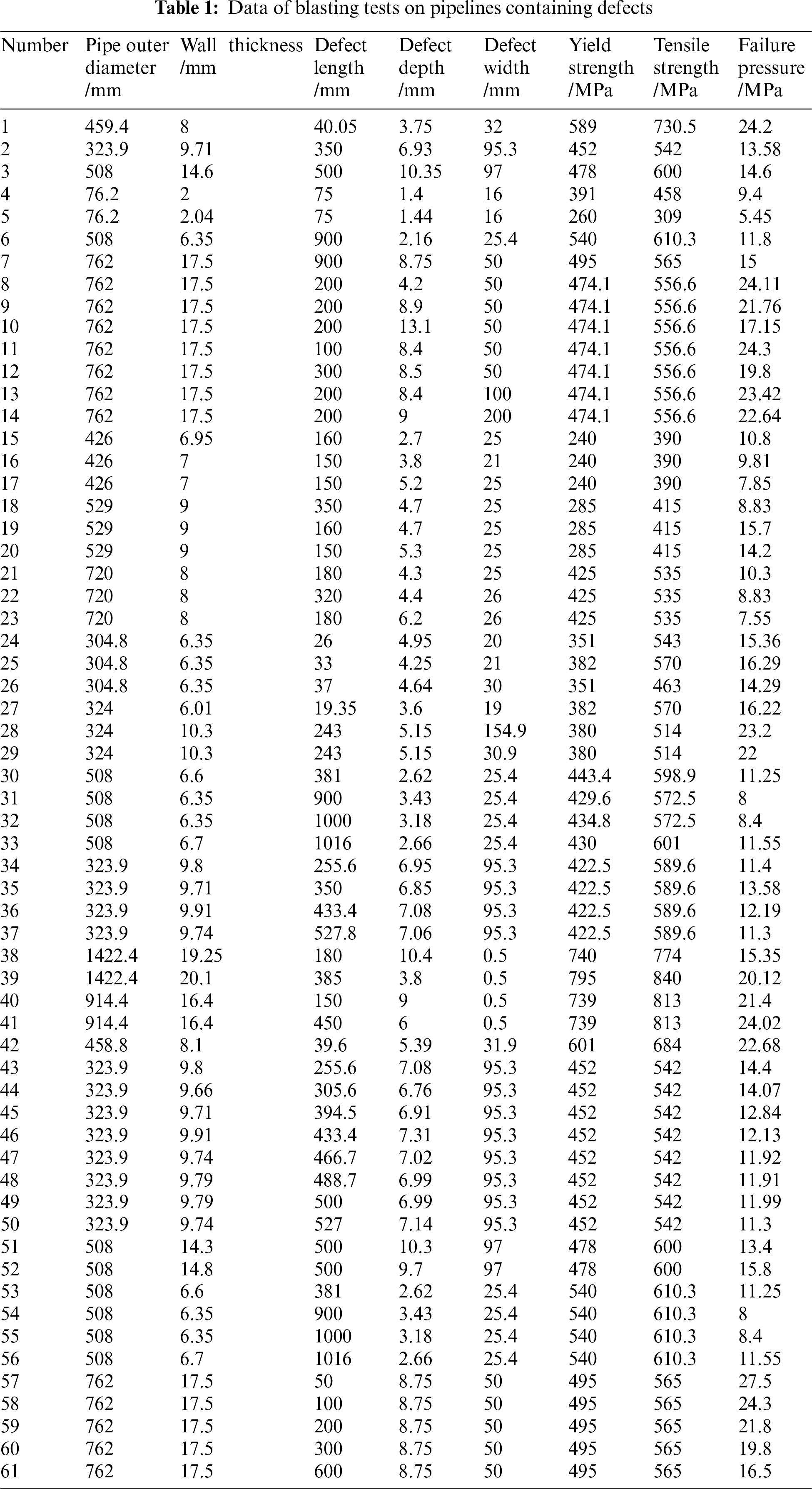
61 groups of experimental data of pipe blasting with defects are selected in reference [9]. Each group of data includes 8 types: Pipe outer diameter, Wall thickness, Defect length, Defect depth, Defect width, Yield strength, Tensile strength, and Failure pressure. 45 groups of data are randomly selected for learning and training, and the remaining 16 groups of data are used to verify the prediction effect of the model. The experimental data of pipeline blasting with defects are shown in Table 1.

4.2 Model Parameter Setting

4.2.1 BPNN Model Parameter Setting

BPNN model adopt a three-layer network structure, with training times of 1000, a learning rate of 0.01, and a minimum error of training target of 0.0001. The network input layer is the factors that affect the failure pressure of the pipeline, so the number of neurons in the input layer is 7; The output layer is pipeline failure pressure, so the number of neurons in the output layer is 1; The hidden layer’s neuronal number is determined according to Eq. (11). The optimal hidden layer’s neuronal number is determined by the trial value, and the trial value results are shown in Fig. 3.

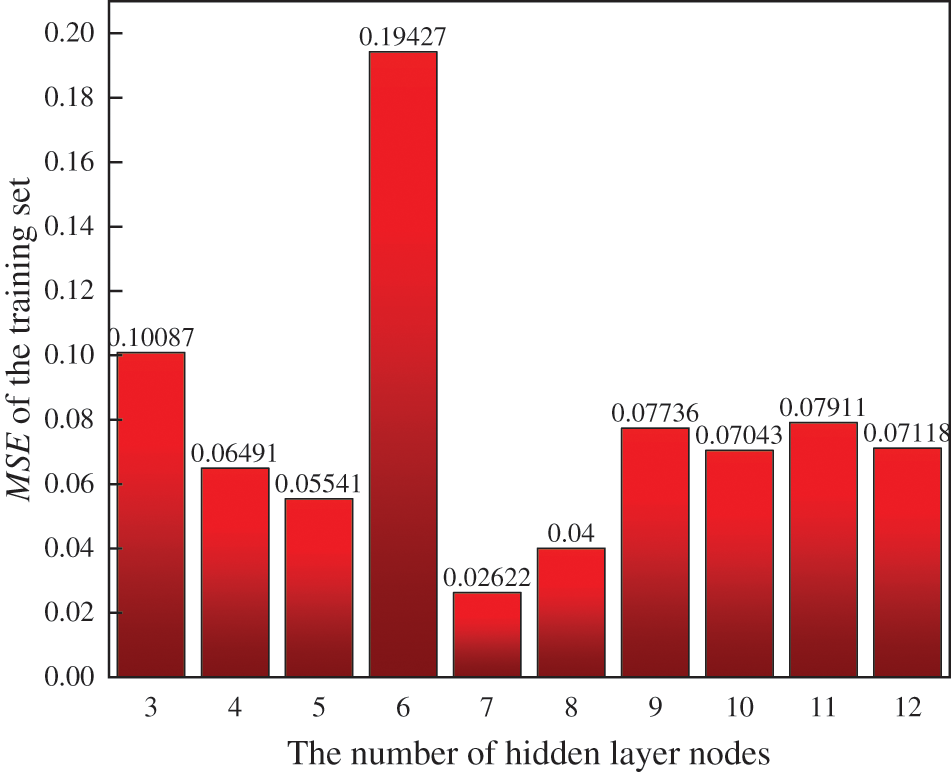
Figure 3: The MSE of the training set at different H values

H=m+n+a(11)

where: H is the hidden layer’s neuronal number, m is the input layer’s neuronal number, n is the output layer’s neuronal number, and a is an integer between 1 and 10 [15]. Therefore, the value range of H is 3~12.

As can be seen from Fig. 3, when the number of neurons in the hidden layer is 7, the mean square error of the corresponding training set reaches the minimum, and its value is 0.02622, so the optimal number of neurons in the hidden layer is 7.

4.2.2 Optimize Algorithm Parameter Setting

From the above analysis, it can be seen that the BPNN model’s network structure is 7-7-1. The optimization algorithm’s initialization parameter settings are shown in Table 2. Among them, the fitness curve of the ISSA-BPNN model in training is shown in Fig. 4.

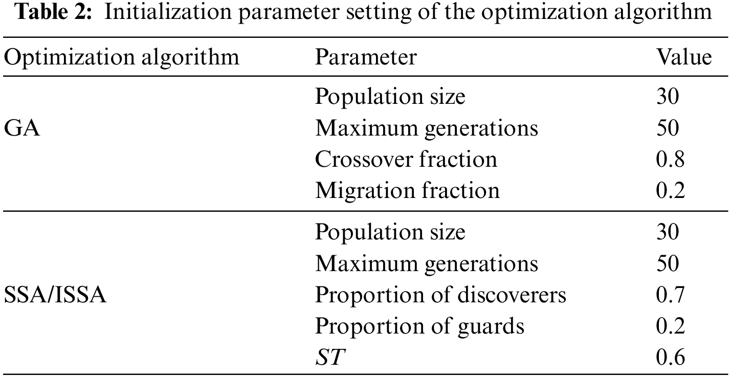
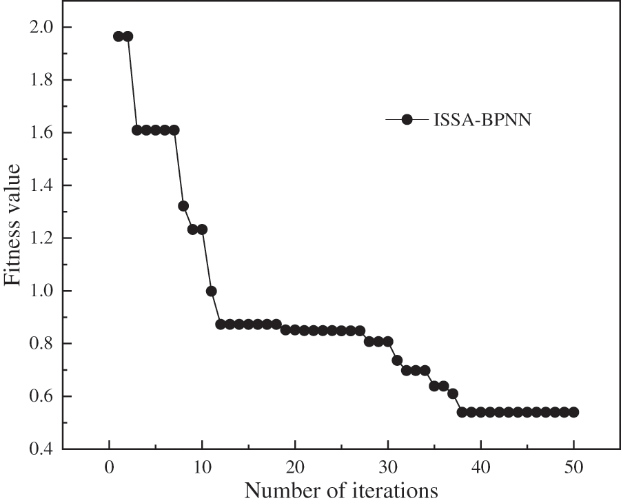
Figure 4: Convergence curve of ISSA-BPNN fitness

4.3 Model Forecast Results and Analysis

The prediction results of BPNN, GA-BPNN, SSA-BPNN, and ISSA-BPNN models for pipeline failure pressure are shown in Table 3 and Fig. 5, and the relative error is shown in Fig. 6. The results show that the predicted results of ISSA-BPNN model are closer to the experimental values than those of the other models. Compared with the single BPNN model, the error interval of the BPNN model optimized by the algorithm is greatly reduced, which improves the overall prediction accuracy of the model.

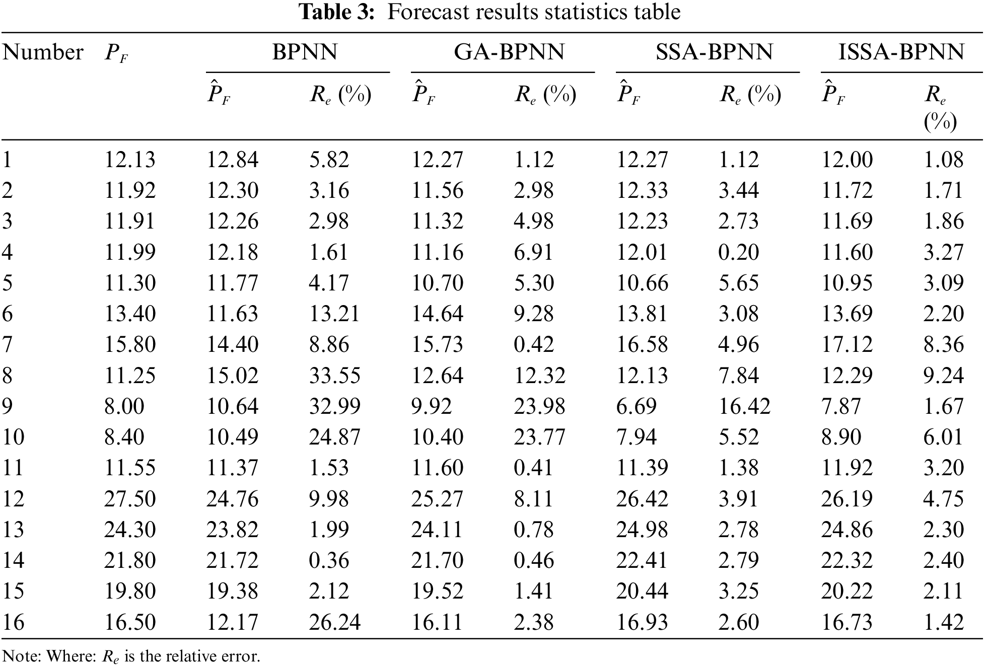
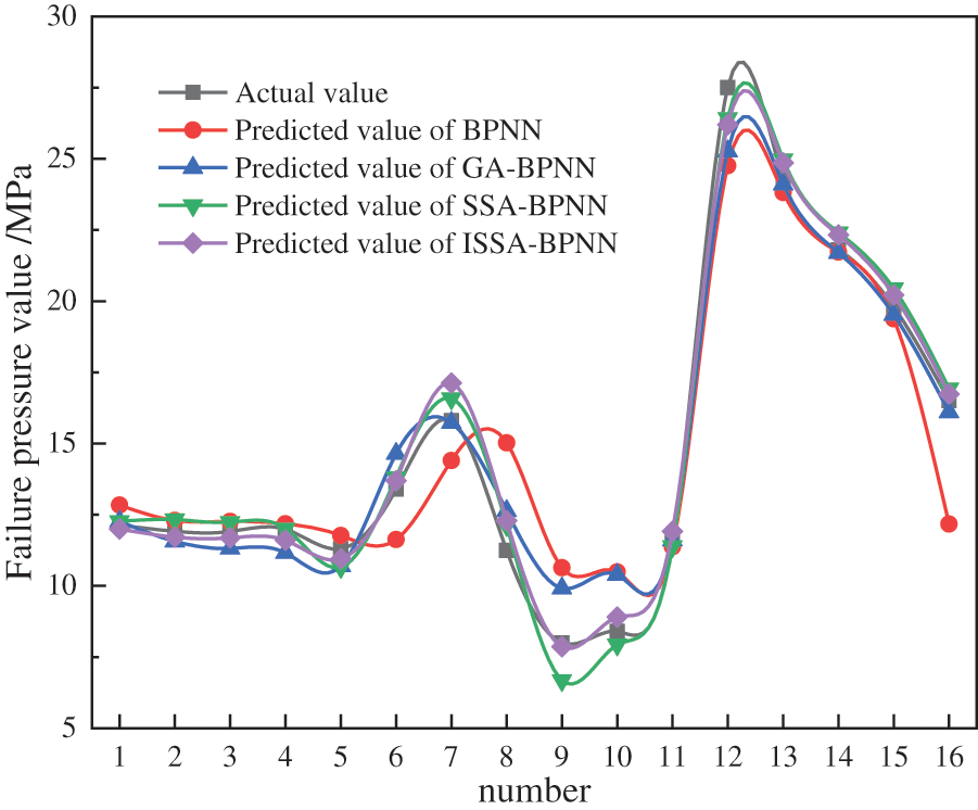
Figure 5: Comparison of model prediction results

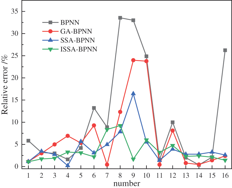
Figure 6: Relative error of prediction results

The above evaluation indicators evaluate the prediction effect of 4 pipeline failure pressure models (BPNN, GA-BPNN, SSA-BPNN, and ISSA-BPNN), and the results are shown in Table 4 and Figs. 7–10. The prediction accuracy of BPNN model is the lowest, MAE, RMSE, MAPE, and R2 are 1.3755, 1.9107, 10.8404% and 0.8895%, respectively, which are the worst among the prediction models. After the BP network is optimized by GA, SSA and ISSA, the prediction error is obviously reduced. Among them, ISSA-BPNN model has the best prediction effect, and its MAE, RMSE, MAPE, and R2 are 0.5002, 0.6240, 3.4177% and 0.9980%, respectively, which are the best prediction models. Compared with the SSA-BPNN model, the ISSA-BPNN model has further improved in error size, dispersion degree, and prediction accuracy. It is proved that the introduction of a Logistic chaotic map really improves the quality of the initial sparrow algorithm population solution, and effectively improves the global search ability and prediction performance of the algorithm.

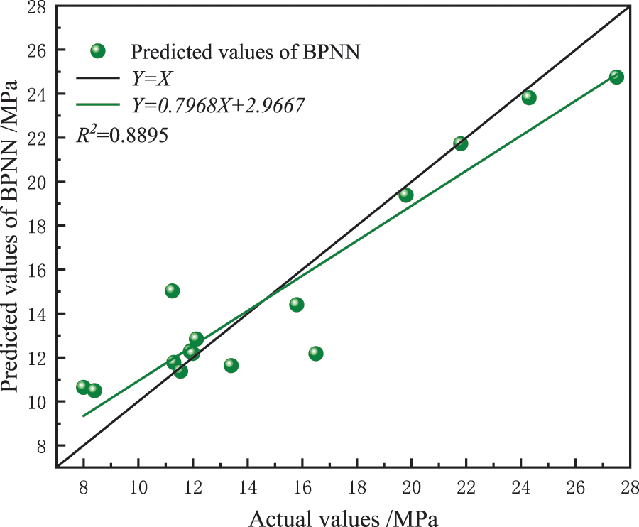
Figure 7: BPNN prediction results in linear fitting graph

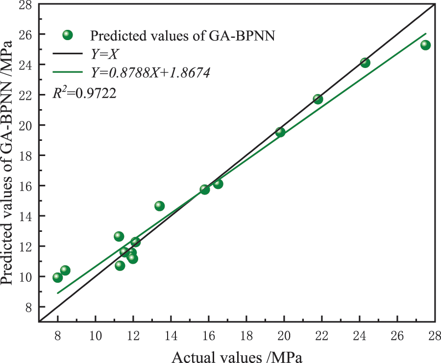
Figure 8: GA-BPNN prediction results in linear fitting graph

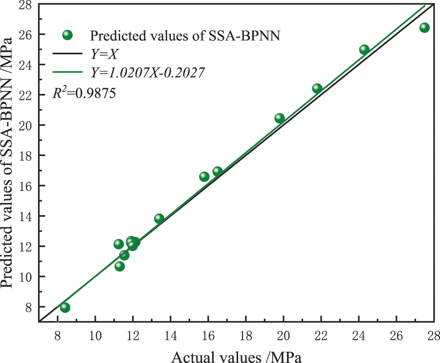
Figure 9: SSA-BPNN prediction results in linear fitting graph

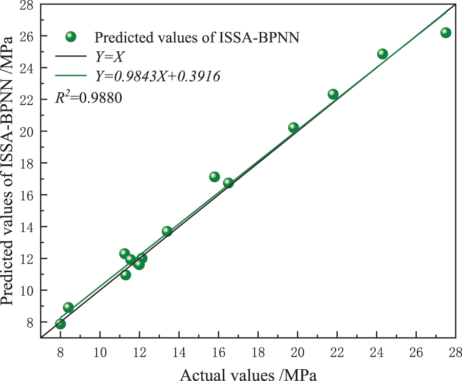
Figure 10: ISSA-BPNN prediction results in linear fitting graph

5  Conclusion

The fundamental prediction model in this research is BPNN, which is optimized using a variety of optimization techniques and models that are established. Using a model that takes into account seven factors that affect the pipeline’s failure pressure, the failure pressure is predicted based on 61 sets of experimental data of pipeline blasting. The following is a summary of the research’s results:

(1) The population of SSA is initialized by a Logistic chaotic map strategy, and ISSA is established. The ISSA algorithm is used to optimize the weights and thresholds of the BP neural network, and the ISSA-BPNN pipeline failure pressure prediction model is established.

(2) By comparing four kinds of pipeline failure pressure prediction models, the performance order is as follows: BPNN < GA-BPNN < SSA-BPNN < ISSA-BPNN. Among them, the MAPE of the ISSA-BPNN model is 3.4177%, and the R2 is 0.9880, both of which are superior to its comparison model. It proves that the ISSA-BPNN prediction model has high accuracy and strong robustness, and this model can provide support for pipeline inspection and maintenance.

Acknowledgement: Thanks are due to the editors and reviewers for their valuable opinions, which are of great help to improve the quality of this paper.

Funding Statement: The authors received no specific funding for this study.

Author Contributions: Study conception and design: Qi Zhuang. Data collection: Dong Liu and Zhuo Chen. Results analysis and interpretation: Qi Zhuang and Dong Liu. All authors reviewed the results and approved the final version of the manuscript.

Availability of Data and Materials: 61 sets of experimental data of pipeline blasting with defects come from reference [9]. https://doi.org/10.1016/j.oceaneng.2019.106497.

Conflicts of Interest: The authors declare that they have no conflicts of interest to report regarding the present study.

References

1. Chen, C., Li, C., Reniers, G., Yang, F. Q. (2021). Safety and security of oil and gas pipeline transportation: A systematic analysis of research trends and future needs using WoS. Journal of Cleaner Production, 279, 1–13. [Google Scholar]

2. Gao, J., Tian, Y., Han, K. J. (2021). Status quo and construction development trend of China’s four major oil and gas channels. China Oil & Gas, 28(6), 41–47. [Google Scholar]

3. Miao, X. Y., Zhao, H., Gao, B. X., Song, F. L. (2023). Corrosion leakage risk diagnosis of oil and gas pipelines based on semi-supervised domain generalization model. Reliability Engineering and System Safety, 238, 1–10. [Google Scholar]

4. Dao, U., Sajid, Z., Khan, F., Zhang, Y., Tran, T. (2023). Modeling and analysis of internal corrosion induced failure of oil and gas pipelines. Reliability Engineering and System Safety, 234, 1–15. [Google Scholar]

5. Lam, C. Z. W. (2016). Statistical analyses of incidents on onshore gas transmission pipelines based on PHMSA database. International Journal of Pressure Vessels and Piping, 145, 1–11. [Google Scholar]

6. Seyed Saleh, M., Ali Shaghaghi, M. (2020). Failure pressure estimation error for corroded pipeline using various revisions of ASME B31G–ScienceDirect. Engineering Failure Analysis, 109, 1–14. [Google Scholar]

7. Bao, J., Zhou, W. (2020). Influence of the corrosion anomaly class on predictive accuracy of burst capacity models for corroded pipelines. International Journal of Geosynthetics and Ground Engineering, 6(4), 1–12. [Google Scholar]

8. British Standards Institution (2007). Guide to methods for assessing the acceptability of flaws in metallic structures, vol. 165, pp. 1–11. Bs7910 British Standards. [Google Scholar]

9. Gao, J., Yang, P., Li, X., Zhou, J., Liu, J. K. (2019). Analytical prediction of failure pressure for pipeline with long corrosion defect. Ocean Engineering, 191, 106491–106497. [Google Scholar]

10. Chen, Y. F., Zhang, H., Zhang, J., Liu, X. B., Li, X. et al. (2015). Failure assessment of X80 pipeline with interacting corrosion defects. Engineering Failure Analysis, 47, 67–76. [Google Scholar]

11. Huang, Y., Qin, G. J., Hu, G. (2022). Failure pressure prediction by defect assessment and finite element modelling on pipelines containing a dent-corrosion defect. Ocean Engineering, 262(2), 1–14. [Google Scholar]

12. Liu, P., Han, Y., Tian, Y. (2021). Residual strength prediction of pipeline with single defect based on SVM algorithm. Journal of Physics Conference Series, 1944(1), 012019. [Google Scholar]

13. Jiang, J. X., Zhang, H., Zhang, D., Ji, B. L., Wu, K. et al. (2022). Fracture response of mitred X70 pipeline with crack defect in butt weld: Experimental and numerical investigation. Thin-Walled Structures, 177, 1–11. [Google Scholar]

14. Jiang, S. Q., Shi, B. (2023). Prediction of failure pressure of corroded pipeline based on ISSA-ELM model. Hot Working Technology, 52(12), 70–75. [Google Scholar]

15. Xu, L. S., Ling, X., Ma, J. J., Ma, H. Q., Fu, X. H. (2021). Prediction on failure pressure of pipeline containing corrosion defects based on DE-BPNN. Journal of Safety Science and Technology, 17(3), 91–96. [Google Scholar]

16. Zhang, T. Y., Shuai, J., Shuai, Y., Hua, L. Y., Xu, K. et al. (2023). Efficient prediction method of triple failure pressure for corroded pipelines under complex loads based on a backpropagation neural network. Reliability Engineering and System Safety, 231, 1–12. [Google Scholar]

17. Li, X. L., Jing, H. M., Liu, X. Y., Chen, G. T., Han, L. F. (2023). The prediction analysis of failure pressure of pipelines with axial double corrosion defects in cold regions based on the BP neural network. International Journal of Pressure Vessels and Piping, 202, 104907. [Google Scholar]

18. Rumelhart, D. E., Hinton, G. E., Williams, R. J. (1986). Learning internal representation by back-propagation errors. Nature, 323, 533–536. [Google Scholar]

19. Xue, J., Shen, B. (2020). A novel swarm intelligence optimization approach: Sparrow search algorithm. Systems Science & Control Engineering, 8(1), 22–34. [Google Scholar]

20. Zheng, Y. Z., Li, L., Qian, L., Cheng, B. S., Hou, W. B. et al. (2023). Sine-SSA-BP ship trajectory prediction based on chaotic mapping improved sparrow search algorithm. Sensors, 32(2), 704. [Google Scholar]