Numerical Simulation Method of Meshless Reservoir Considering Time-Varying Connectivity Parameters

1  Introduction

In strong edge and bottom water reservoirs and waterflood reservoirs, with the extension of development time, the physical properties of reservoirs have changed significantly compared with the original state due to long-term water erosion [1–5]. Among the changes in reservoir properties, permeability variation is one of the most common phenomena. It has a significant impact on reservoir production efficiency, displacement performance, and oil-water distribution [6–10]. To date, many scholars have conducted exploratory research on the time-varying characteristics of permeability. The main characterization methods can be divided into two categories.

The first is the field statistical and laboratory experimental methods. Liu [10] made a statistical regression of the mathematical relationship between permeability change ratio and waterflood erosion ratio based on 200 physical simulation experiments of core samples at different water-bearing stages. Hong et al. [11] studied the dynamic variation law of permeability in high and low permeability reservoirs during the flooding process and concluded that the permeability variation in waterflood reservoirs can be expressed using a logarithmic formula. This method can provide actual field data and controlled experimental conditions, ensuring the accuracy of the theoretical model. However, deriving precise results usually requires significant time and resource investment, and the differing conditions of various fields or laboratories may limit the general applicability of the research.

The second is the numerical simulation metho. Xu et al. [12] analyzed the changing relationship between reservoir wettability and permeability under different waterflood multiples through pore-level seepage simulation. Tian et al. [13] improved the convection-solid coupling algorithm by considering the different seepage characteristics in particles, between particles, and between fractures. This algorithm is used to simulate the permeability of heat-treated granite samples under different confining pressure conditions. The numerical simulation method offers strong flexibility and controllability, enabling large-scale parameter sensitivity analysis to be conducted in a relatively short time. However, the simulation results often need to be verified by field data, and the reliability and applicability need to be tested by long-term practice. To facilitate the effective combination of time-varying permeability and reservoir numerical simulation methods, this paper adopts a time-varying permeability characterization method based on field statistical regression.

Currently, numerous scholars have taken into account the time-varying mechanisms of properties like permeability. By integrating these considerations with grid-based numerical simulation methods, they have achieved remarkable advancements in the research on numerical simulation techniques for time-varying reservoir properties [14–17]. Nevertheless, to guarantee computational accuracy, the grid-based numerical simulation methods adopted by these scholars necessitate extensive fine-grid discretization within the reservoir calculation domain. This requirement gives rise to problems such as poor convergence and overly long computation times. In contrast, this paper utilizes the connection element method (CEM) [18–21], which is a meshless method [22–27]. The CEM replaces the traditional grid topology with a flexible node representation, enabling the reservoir to be modeled as a flow network. This network is composed of one-dimensional connection elements, which are characterized by transmissibility and connection volume. On this basis, the influence of time-varying permeability characteristics on transmissibility is thoroughly considered, resulting in a meshless numerical simulation method that accounts for the time-varying features of connection parameters.

2  Time-Varying Mathematical Model

2.1 Basic Assumptions

In establishing the meshless model, the fundamental assumptions include the consideration of oil-water two-phase flow under adiabatic conditions, where thermal exchange with the environment is disregarded. The effects of gravity and capillary forces are neglected to simplify the multiphase flow dynamics, as capillary pressure exerts negligible effects on macroscopic production data (e.g., water cut, pressure distribution) during waterflooding simulations in medium-to-high permeability reservoirs. Additionally, the viscosities of the fluids are assumed to remain constant throughout the simulation, independent of variations in pressure or temperature. The temporal variation in permeability is modeled using a logarithmic formulation derived from statistical regression of field data, which provides an empirical representation of the dynamic changes in reservoir properties over time. These assumptions collectively aim to balance computational efficiency with the accurate representation of key physical processes in the reservoir system.

2.2 Mathematical Model Construction and Solution

Through the meshless node characterization, the reservoir flow network composed of equivalent one-dimensional connection elements is presented. To calculate the seepage control equation based on the connection element system, the seepage characteristic parameters of the connection element should first be characterized. The transmissibility mainly regulates the time when the oil well reaches water, and its essence is to affect the seepage capacity of the fluid in a single connection element, and then determine the migration efficiency of the fluid in the flow network. The connection volume represents the effective pore volume between individual connection elements, and its size directly affects the productivity level of the well and even the block. As two core parameters of connection meta-model, transmissibility and connection volume play a key role in model derivation and calculation, and profoundly affect the prediction accuracy of the model. Because the pore volume changes with the development time is small, the permeability parameter with more obvious time-varying characteristics is selected in this paper. According to the permeability changes with the change of face flux, the transmissibility is calculated.

Based on the above assumptions, the mass conservation equation for the model is established as follows [16]:

∑k=1Nl∑j=1NwTijk(pj(t)−pi(t))+qi(t)=dpi(t)dt∑k=1NlCt,kVp,i,k(t)(1)

where, Nw is the number of Wells connected to well i on layer k; qi(t) is the inflow and outflow of source and sink phase from well i under reservoir conditions; pi is the average pressure of the connection element Vp,i; Ct,k is the comprehensive compression coefficient of well i on layer k.

Traditional CEM construct models based on static parameters, assuming that reservoir geological parameters remain constant during development. This approach neglects the time-varying characteristics of connectivity transmissibility and connection volume in its derivation. Areal flux, defined as the cumulative water phase volume passing through a unit area, effectively characterizes the flushing intensity in oilfields during high-water-cut production stages. Following Zhao Hui’s connection element theory, the authors propose permeability corrections in the formula based on its variation pattern with areal flux, subsequently incorporating the modified permeability into connectivity transmissibility calculations.

Tij=αλijKijVp,i∑m=34em,ji(2)

where, Tij is defined as transmissibility of the conduction element (i,j); α is the unit conversion factor; λij is the average mobility of the connection element; Kij is defined as the average permeability of connection elements; Vp,i is the node control volume, and em,ji is the element in the contribution matrix obtained by expanding and calculating node j as the central node.

Through field data statistics and regression analysis, it was found that the permeability ratio showed a good logarithmic correlation with the surface flux [11]:

K′=Kij(aln⁡M+b)(3)

where, K′ is the permeability after change; Ki is the initial permeability; a and b are regression coefficients, which are related to reservoir cementation strength, permeability, crude oil viscosity, oil production rate and pressure drop rate; M is the face flux.

The equation to obtain the coefficients a and b is:

a=0.0014Kij−0.2183,b=−0.0041Kij+1.3647(4)

Combined with the permeability variation rule, the expression for the transmissibility is:

Tij=((0.0014Kij−0.2183)ln⁡QijLijVp,ij+(−0.0041Kij+1.3647))αλijKijVp,i∑m=34em,ji(5)

where, Tij represents the transmissibility of the connection element (i,j); Kij is the average permeability of the connection element, Qij is the flow rate through the connection element, Lij is the distance between the two nodes (connection element), Vij is the control volume of the connection element, α is the unit conversion factor, λij is the average mobility of the connection element, Vi is the control volume of node i, em,ji is the element of the contribution matrix calculated with node i as the central node.

By substituting Eqs. (5) into (1) and combining with the permeability variation rule, the difference scheme of the modified multilayer reservoir mass conservation equation can be obtained as follows:

∑k=1Nl∑j=1Nw[[(0.0014kijk−0.2183)ln⁡QijkLijkVijk+(−0.0041kij+1.3647)]αλijkijVi∑m=34em,ji(pj(t)−pi(t))+qi(t)=dpi(t)dt∑k=1NlCt,kVp,i,k(t)(6)

By discretizing Eq. (5), the solution for pressure can be obtained. Combining this with the pure convection equation allows for the dynamic changes in water cut and oil production to be determined [16].

The proposed methodology introduces non-traditional grid elements to define novel control volumes and productivity indices for global coarse-scale nodal pressure calculation. A graph-theory-based pruning strategy is applied to eliminate low-flux connections, while semi-analytical solutions are implemented at local fine scales to resolve multiphase saturation and polymer concentration distribution in polymer flooding reservoirs. This approach enables rapid computation of pressure, production rates, and water cut [16].

2.3 Model Validation

In this section, a three-layer meshless conceptual model with five injectors and four producers was constructed to validate the accuracy and applicability of the numerical simulation method incorporating time-varying connectivity parameters under varying permeability conditions. The connectivity network of the model is illustrated in Fig. 1a, while the initial parameter configurations are summarized in Table 1. The value of face flux M can be calculated by multiplying the cumulative fluid volume through the connection element by the water injection allocation factor, followed by multiplying the resultant value by the ratio of connection element length to connection volume. The water injection allocation factor is schematically illustrated in Fig. 1b.

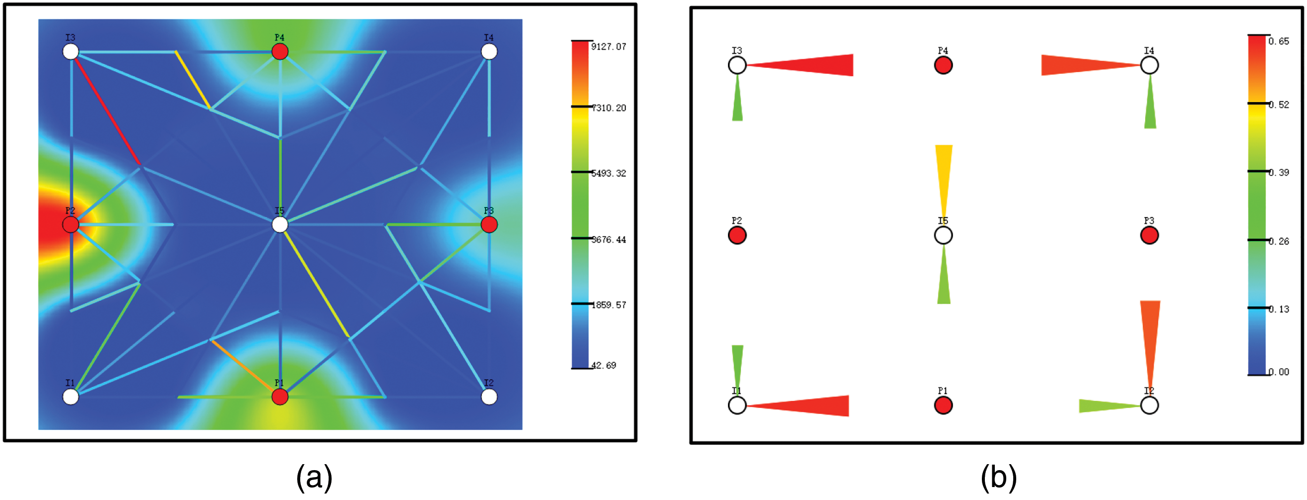
Figure 1: Diagram of conceptual model. (a) Permeability field and flow betwork superimposed diagram; (b) Water injection split factor diagram

Based on this model, three verification cases are used for numerical simulation, as shown in Table 2.

Based on this model, numerical simulations were performed using three verification cases, with detailed descriptions presented in Table 2. The permeability distribution and connection transmissibility at the final time for Case 1, Case 2, and Case 3 are illustrated in Figs. 2 and 3, while the comparison of cumulative oil production and water cut is shown in Fig. 4.

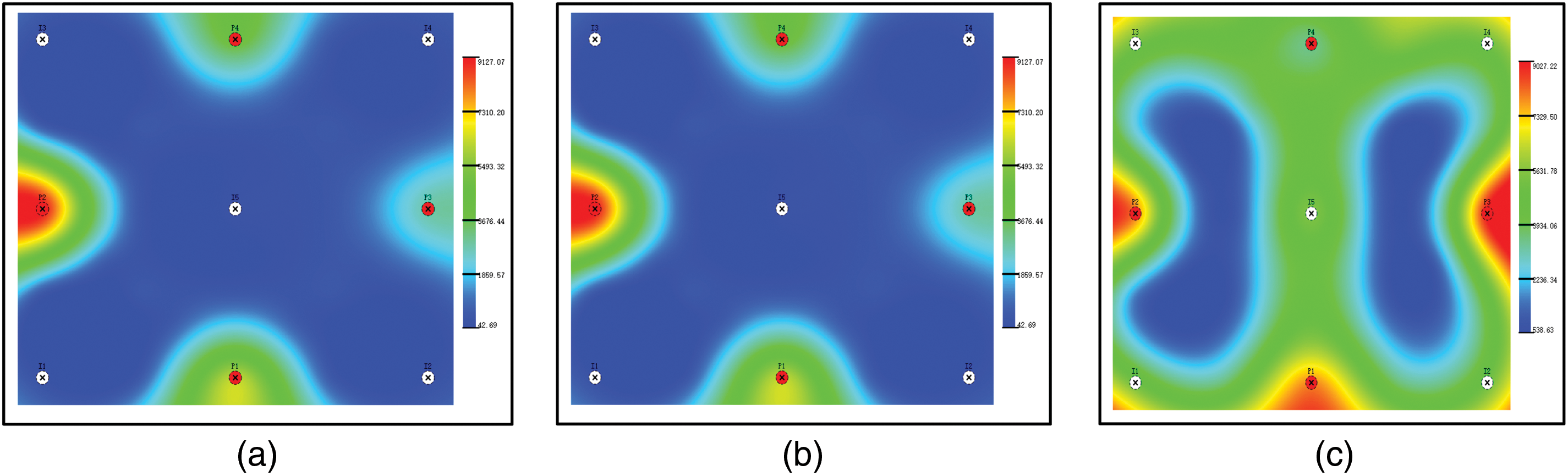
Figure 2: The permeability of the three cases of the final moment. (a) The permeability of Case 1; (b) The permeability of Case 2; (c) The permeability of Case 3

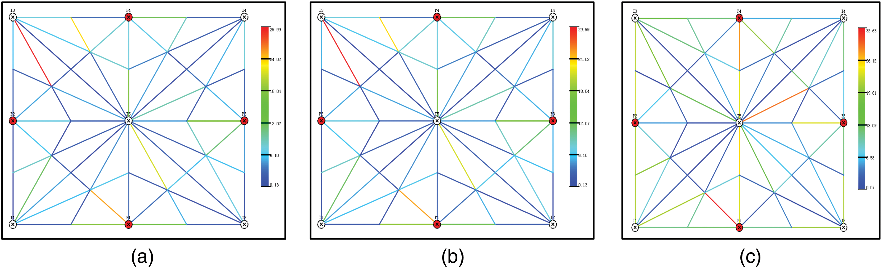
Figure 3: The connection transmissibility of the three cases of the final moment. (a) The connection transmissibility of Case 1; (b) The connection transmissibility of Case 2; (c) The connection transmissibility of Case 3

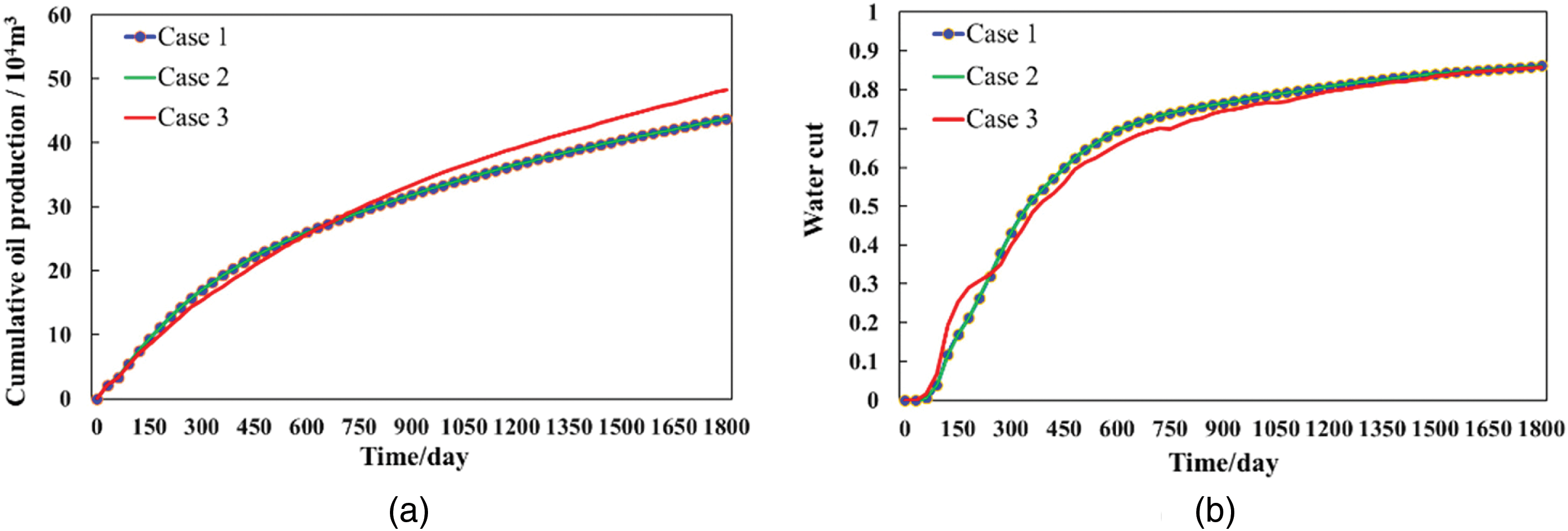
Figure 4: Diagram of comparison curves of calculation results of the three cases. (a) Cumulative Oil Production; (b) Water Cut

A comparison of the results between Case 1 and Case 3 reveals that when the time-varying characterization formula for permeability is incorporated and the permeability change factor is set to 1, the calculated connection conductivities and dynamic results of Case 3 align perfectly with those of the static parameter model, validating the accuracy of formula derivation and model construction. Additionally, the final connection conductivity calculated for Case 3 better matches the permeability field distribution. Compared with Case 1, Case 3 shows an increase of 16,700 cubic meters in oil production and a 0.36% reduction in water cut. These findings indicate that accounting for time-varying characteristics in Case 3 leads to distinct production dynamics, confirming that reservoir time-variation significantly impacts numerical simulation results and warrants further in-depth research.

2.4 Sensitivity Analysis

In this section, the influence of single-factor parameter changes on the model is mainly analyzed. The sensitivity analysis of the model parameters mainly studies the influence of different injection rates and initial permeability on the daily oil production and water cut of a single well and block. The above mechanism model is modified into a homogeneous model with the same physical properties, such as permeability and porosity of each node, and the model parameters are adjusted according to different influencing factors. When sensitivity analysis is performed for any of the above parameters, the remaining parameters remain unchanged.

2.4.1 Injection Rate

To analyze the impact of injection intensity on oil production and water cut variations, daily water injection rates were set to 150, 200, 250 and 300 m3/d, with constant initial permeability and time-varying regression coefficients. The specific parameter configurations for each scenario are summarized in Table 3. Numerical simulation results (Fig. 5) indicate that as the injection rate increases from 150 to 300 m3/d, the oil production rises from 402.0 × 103 to 501.2 × 103 m3, demonstrating a progressive enhancement in cumulative block oil production with higher injection intensity. Concurrently, the block water cut increases from 90.16% to 92.59%, confirming a positive correlation between water injection intensity and water cut. The daily oil production curves of individual wells under the highest injection intensity exhibit a sharp decline in productivity after an initial peak during the early development phase. Although high injection intensity achieves rapid oil production initially, it accelerates water channeling, leading to premature productivity decline. These results suggest that excessive injection intensity, while temporarily boosting short-term production, exacerbates reservoir heterogeneity-driven displacement inefficiency and reduces long-term development effectiveness. To optimize field development, a balanced strategy integrating production targets and water cut control is essential. Practical measures such as profile control and water shutoff technologies should be implemented to improve displacement efficiency. Additionally, dynamic monitoring and timely adjustments to injection-production parameters are critical to maintaining stable and efficient reservoir performance. Notably, under high-intensity water injection, intense hydrodynamic scouring forms preferential flow pathways, allowing injected water to break through to production wells while bypassing oil-rich zones. Moreover, increased injection rates elevate the volumetric flux, amplifying permeability alteration ratios and intensifying the sensitivity of production dynamics to injection intensity. Although high injection rates may temporarily enhance oil recovery rates, they risk triggering ineffective fluid cycling over the long term, potentially accelerating cumulative oil decline.

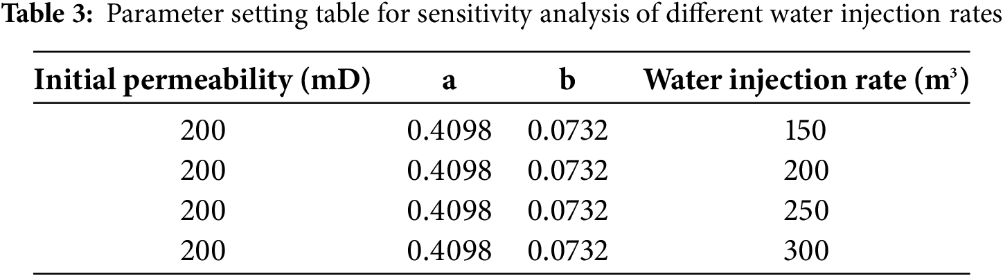
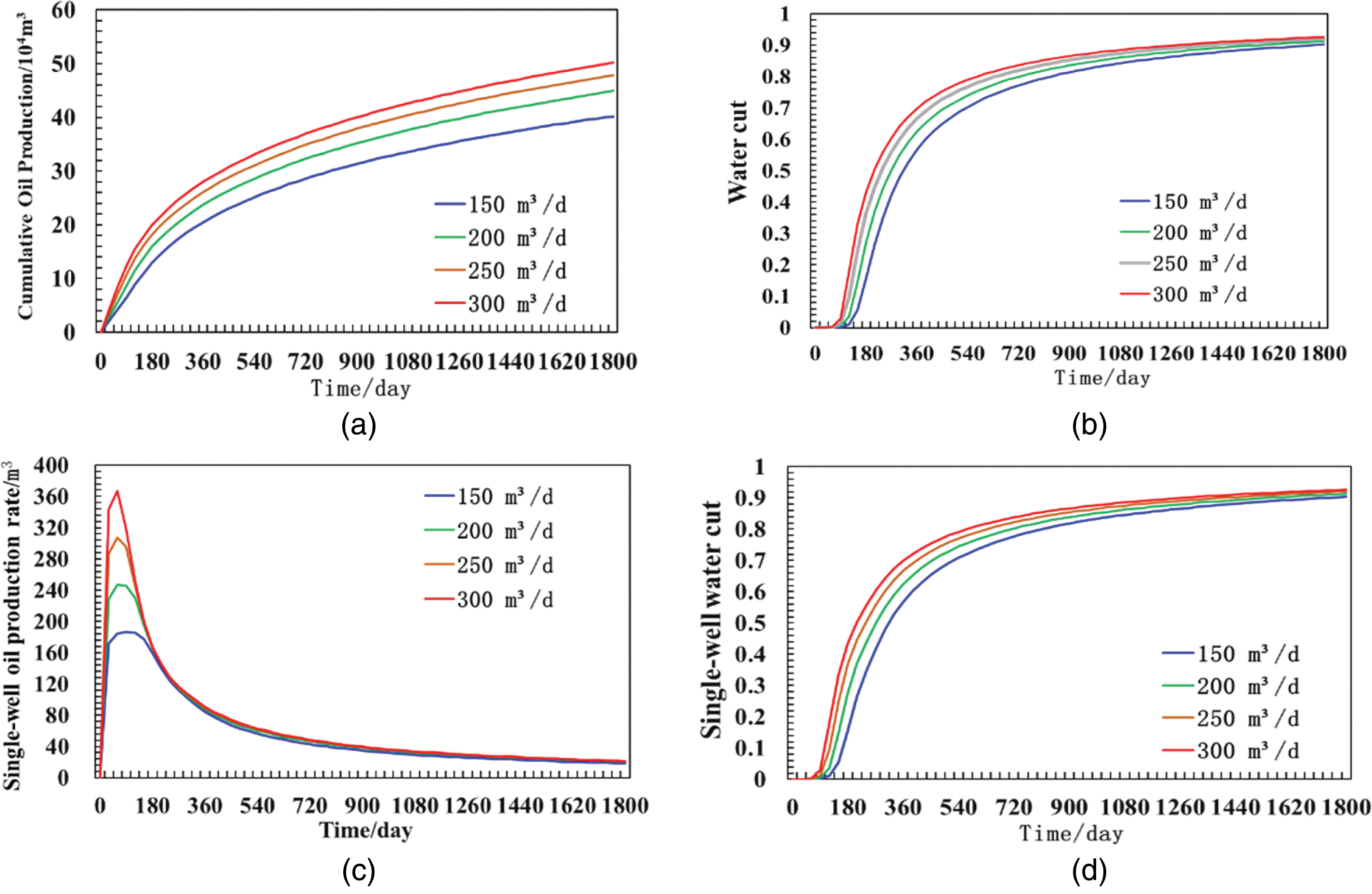
Figure 5: Production dynamic curves under different water injection rates. (a) Cumulative Oil Production; (b) Water cut; (c) Single-well oil production rate; (d) Single-well water cut

2.4.2 Initial Permeability

To analyze the variations in oil production and water cut for individual wells and the entire block under different initial permeabilities, the model’s initial permeability was set to 200, 400, 600, and 800 mD, respectively. Table 4 presents the specific parameter settings for permeability, regression coefficients, and water injection rate in the sensitivity analysis cases. As indicated by the data, the transmissibility increases progressively with higher initial permeability. This trend aligns with the transmissibility calculation formula, confirming a positive correlation between permeability and transmissibility. The production performance comparison curves obtained through time-varying numerical simulation are shown in Fig. 6. Simulation results reveal that the cumulative oil production of the block for the four cases reaches 402.0 × 103, 403.9 × 103, 411.5 × 103, and 419.0 × 103 m3, respectively. The curves further demonstrate that higher initial permeability enhances oil production. Regarding water cut trends, the block-level curves show a rapid increase in water cut during the early stage as permeability rises, followed by stabilization after 1000 days. The final water cuts for the four permeability cases (from low to high) are 90.16%, 89.83%, 89.48%, and 89.01%, respectively. Analysis of the model’s single-well daily oil production indicates that all cases exhibit high efficiency during the initial waterflooding phase, followed by a gradual decline in production rates until stabilization in later stages. Notably, higher permeability accelerates water breakthrough time. The single-well water cut curves exhibit similar trends to the block-level curves, with higher permeability leading to faster water cut increases during the early development phase but lower average water cuts. This phenomenon arises because enhanced oil-phase mobility in homogeneous reservoirs under high-permeability conditions improves well productivity under identical pressure differentials. Simultaneously, elevated permeability accelerates water invasion or injected water breakthrough, resulting in earlier water breakthrough and rapid water cut escalation.

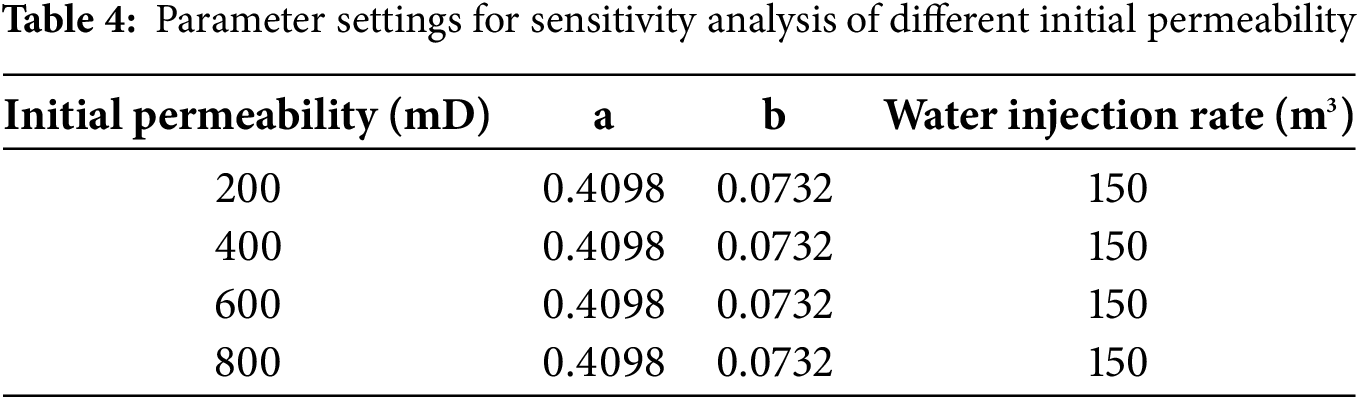
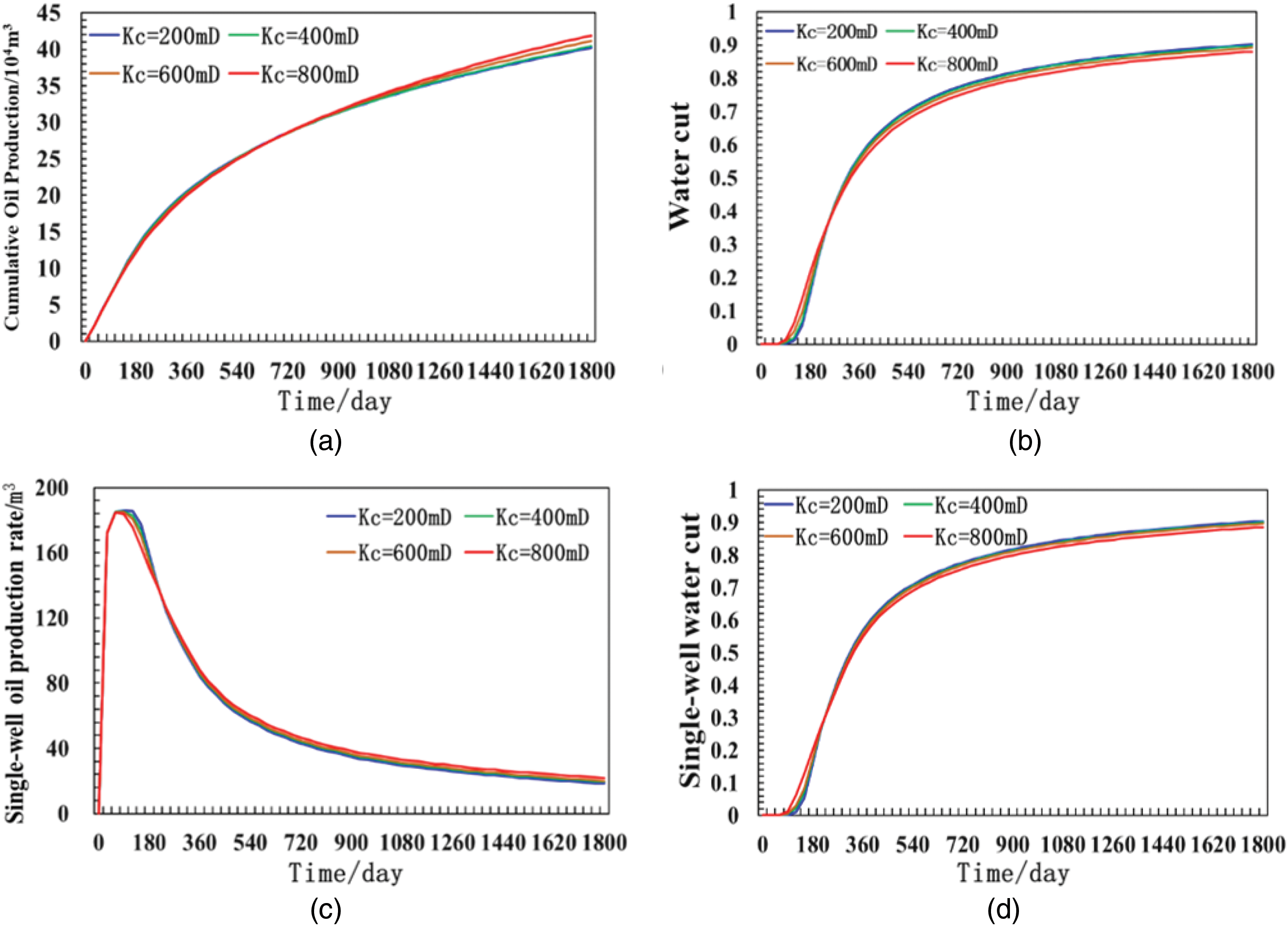
Figure 6: Production dynamic curves under different permeability. (a) Cumulative Oil Production; (b) Water cut; (c) Single-well oil production rate; (d) Single-well water cut

2.4.3 Time-Varying Regression Parameters

Analyze the influence of different regression coefficients on the production dynamics. Set the regression coefficients under different reservoir conditions respectively. The regression coefficients are related to various factors such as the cementation degree of the reservoir, the viscosity of the crude oil, the oil production rate, and the rate of pressure decline. The regression coefficient schemes of the three calculation examples adopted by the author respectively represent three typical reservoir conditions, namely low-permeability reservoirs, medium-permeability reservoirs, and high-permeability reservoirs. The specific selection of regression coefficients and the settings of other constant parameters are shown in Table 5 below, and the comparative curves of the production dynamics of the simulation results are shown in Fig. 7. By comparing the cumulative oil production of the cases, it can be known that the oil production under the condition of low-permeability reservoirs is the lowest, with a production of 391,200 cubic meters. The oil production under the condition of medium permeability is significantly increased, with a production of 397,600 cubic meters. The oil production under the condition of high-permeability reservoirs is the highest, with a production of 402,000 cubic meters. The average water cut of the cases in the three calculation examples is 92.80%, 91.48%, and 90.16%, respectively. From the comparison of the water cut curves of the cases, it can be found that the water cut of the low-permeability reservoir example is relatively low in the initial stage, and the rising speed is slow. However, under the production condition of a constant liquid production rate, the final water cut value ranks first among the three. The water cut of the high-permeability reservoir example increases the fastest in the early stage. Due to the strong fluid seepage ability, the oil production efficiency is high, and the average water cut is relatively low. In the ideal homogeneous model, the residual oil saturation will be lower. There are significant differences in the shape and dynamic characteristics of the daily oil production rate curves of low-permeability reservoirs, medium-permeability reservoirs, and high-permeability reservoirs. The daily oil production of the high-permeability reservoir example reaches its peak rapidly in a short time and then decreases, and finally tends to be stable. The peak values of the oil production rate curves of the medium- and low-permeability reservoir examples decrease successively. The daily oil production of the low-permeability reservoir rises relatively slowly, with the lowest peak value and a later occurrence. The adjustment of the regression parameter scheme has a relatively large impact on the time variation of permeability, and further affects the prediction of the connection conductivity and the production dynamics curve.

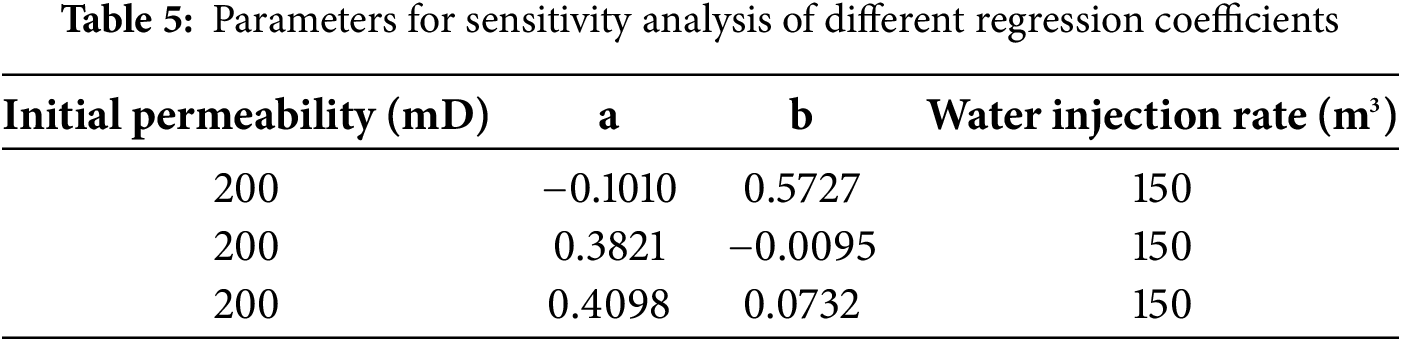
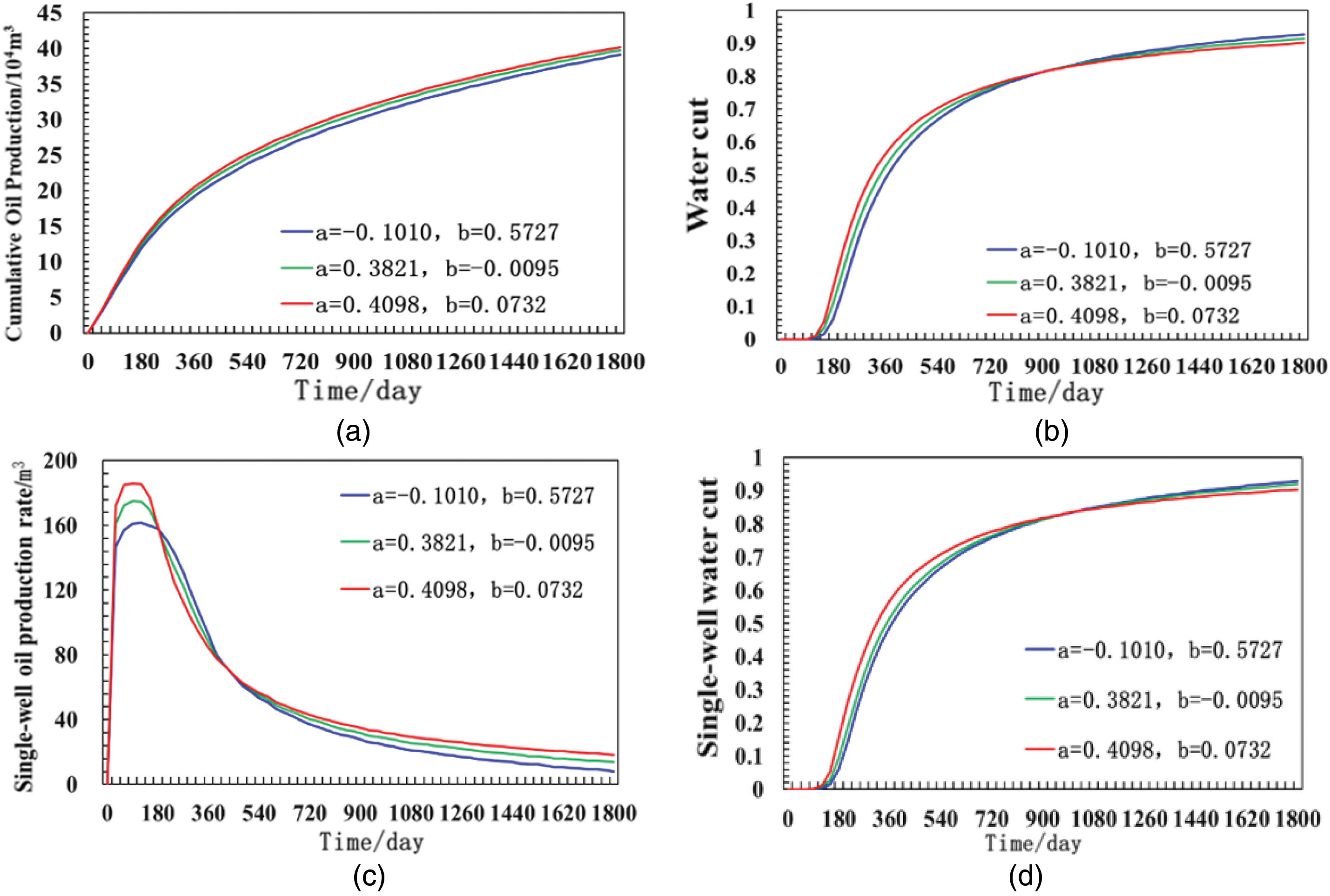
Figure 7: Production dynamic curves under different regression coefficients. (a) Cumulative Oil Production; (b) Water cut; (c) Single-well oil production rate; (d) Single-well water cut

3  Application

3.1 Reservoir Description

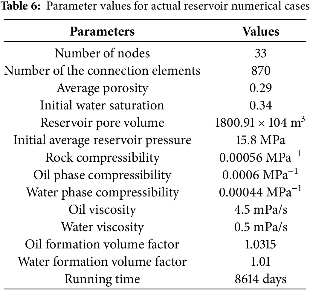
The W oilfield is a high-permeability, water-drive sandstone reservoir. The block contains 33 wells, and the injection-production development period has lasted for 8614 days. The reservoir has now entered a high water-cut stage, with significant water flooding intensity, leading to a substantial variation in reservoir permeability. By employing a numerical simulation method that considers time-varying connectivity parameters, the production dynamics of the reservoir can be predicted more accurately, bringing the simulation results closer to the actual situation.

3.2 Model Construction

The method described in this paper was applied to an actual block of a certain oilfield, and the grid-free model established is shown in Fig. 8. The connectivity network of the model is shown in Fig. 8a, and the initial parameter configuration is shown in Table 6. The water injection allocation coefficient is shown in Fig. 8b.

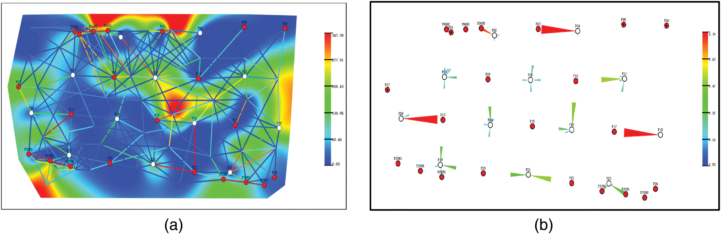
Figure 8: Diagram of the actual model. (a) Permeability field and flow network superimposed diagram; (b) Water injection split factor diagram

The simulation method, considering the time-varying characteristics of the connectivity parameters, is used to predict the production dynamics. The simulation calculation ran for 8614 days, and two dynamic prediction results of block cumulative oil production and block water cut are obtained (as shown in Fig. 9a,b) and compared with the historical data. The results demonstrate that the average accuracy of cumulative oil production in simulation calculations is 87.2% for the numerical simulation method that does not account for the time-varying characteristics of connectivity parameters and 91.1% for the method that does. Similarly, the average accuracy for water cuts is 79.6% and 82.5%, respectively. This indicates that considering the time-varying characteristics of connectivity parameters enhances the accuracy of the simulation, providing a more accurate reflection of the actual geological features and oil-water migration conditions compared to methods that assume constant parameters.

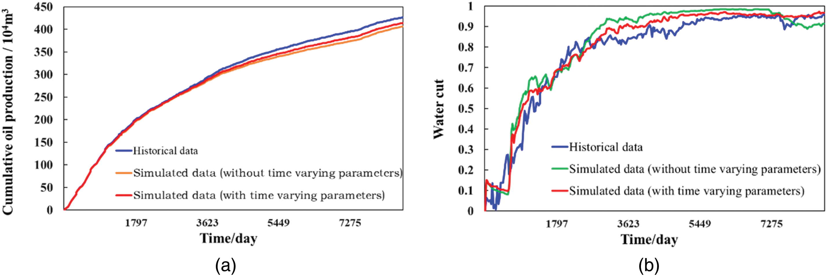
Figure 9: Diagram of block calculation accuracy curve of two simulation methods. (a) Cumulative Oil Production; (b) Water Cut

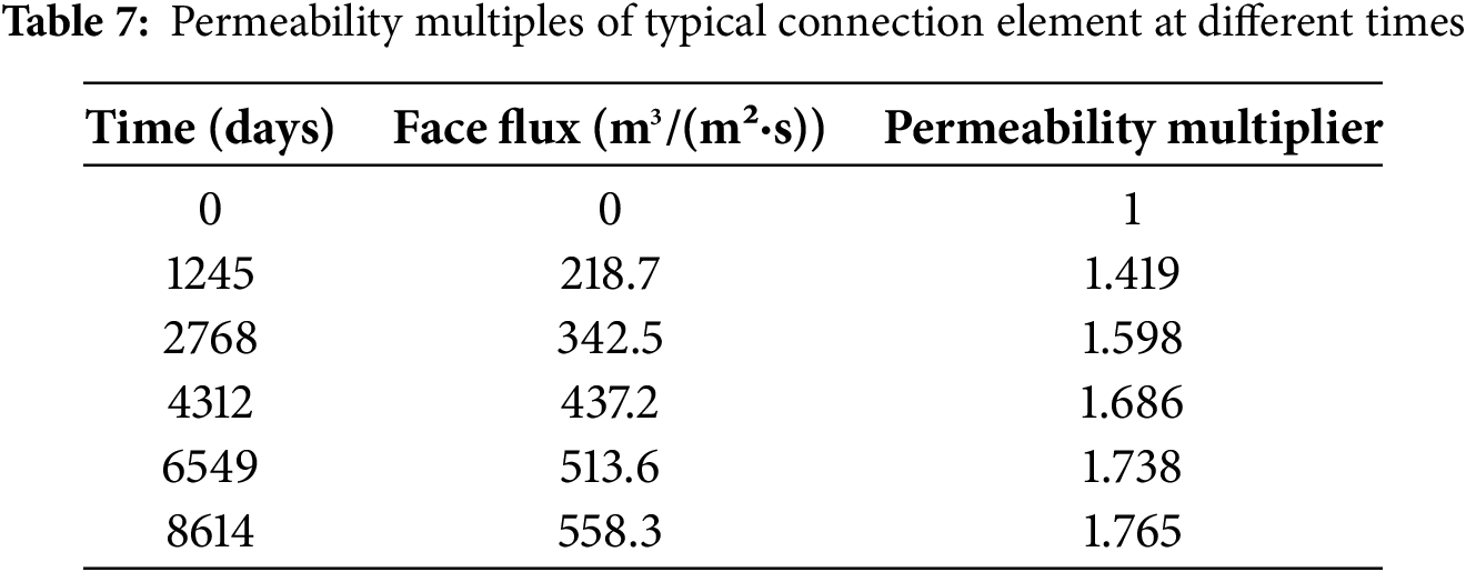
The transmissibility of the static meshless model is shown in Fig. 10a, and the transmissibility of the model considering time variability is shown in Fig. 10b. By comparison, it can be found that the transmissibility of part of the connection element in the time-varying model changes obviously, and the location of the connection element is in the place with a large permeability value. In the model considering time variability, the transmissibility variation in the high permeability region is particularly prominent, which is consistent with the conclusion of the sensitivity analysis. Taking the connection element composed of node P09 and node P10 as the research object, the average permeability of the connection element is 357.4 mD. The face flux of the connection element at different times was calculated based on the distribution of the interlayer waterflood split coefficient, and the permeability multiple at different times was calculated according to the expression of the permeability multiple change rule, as shown in Table 7. By comparing the change multiples of permeability at different times, it can be found that the permeability multiples in the high permeability area show a trend of “first fast and then slow” with the gradual increase of time and face flux. For example, in the initial period (the first 2000 days), the permeability may increase rapidly from 1.0 to 1.4 times, reflecting the rapid transformation of pores or fractures by fluid erosion. In the later period (6000 days), the growth rate gradually slowed down (such as from 1.7 times to 1.8 times), reflecting the dynamic effect approaching saturation.

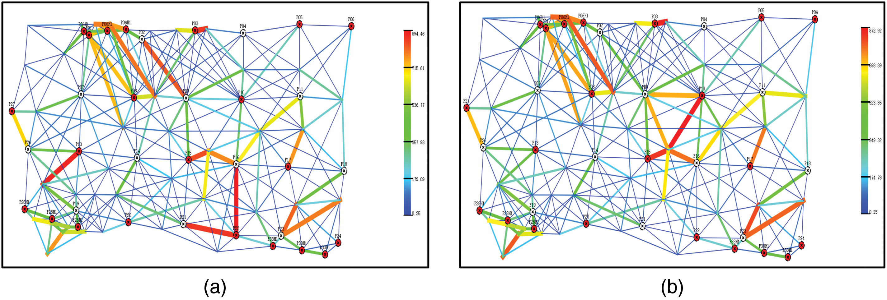
Figure 10: Diagram of connection con of two simulation methods. (a) Static parameter; (b) Time-varying parameter

The oil saturation at the last moment of the static meshless model is shown in Fig. 11a, and the oil saturation at the last moment of the model considering time variability is shown in Fig. 11b. By comparing the final oil saturation of the time-varying model and the static model, it can be found that the remaining oil in the high-permeability region in the dynamic model is significantly reduced, because the permeability increases with the increase of flow, and the displacement is more adequate. The static model may overestimate the remaining oil in the high permeability area because of ignoring the dynamic effect, resulting in a slight deviation in the overall recovery efficiency prediction. This shows that the influence of time variability on development results cannot be ignored, especially when optimizing water injection schemes or evaluating residual oil distribution, dynamic models can guide accurate development.

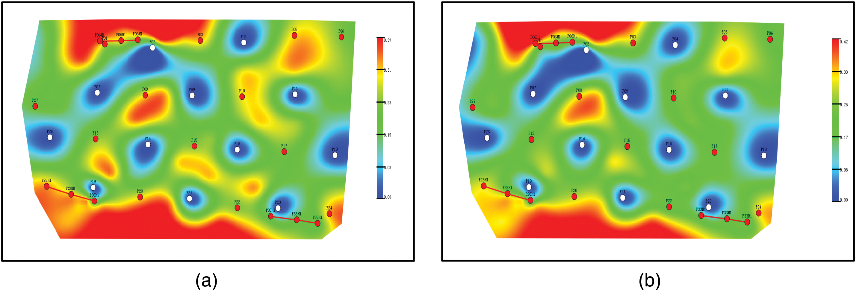
Figure 11: Diagram of oil saturation of two simulation methods. (a) Static parameter; (b) Time-varying parameter

4  Conclusion and Prospect

In this paper, a time-varying numerical simulation method is proposed to consider the dynamic characteristics of the enhanced seepage capacity of the reservoir after long-term water flooding.

1.    Based on the traditional connection-element method, we innovatively introduce the dynamic correlation mechanism of permeability with fluid flow intensity (face flux) and construct a numerical simulation method that can consider the time-varying characteristics of meshless connectivity parameters.

2.    To verify the reliability of the research method, an idealized model was first established in this section, and three simulation schemes were designed for comparison and verification. The results showed that the numerical simulation method model with dynamic parameters significantly improved the prediction accuracy of oil production and water saturation compared with the traditional static simulation method.

3.    The sensitivity analysis of the effects of water injection intensity and initial permeability on production dynamics was carried out, and it was found that the impact of water injection intensity on production dynamics was significant.

4.    The proposed method is applied to real blocks, and the accuracy of cumulative oil production and water cut in blocks is improved by 3.9% and 2.9%, respectively, compared with the traditional connection-element method, which shows that the proposed method can simulate the real oil and water migration and distribution in the reservoir.

Acknowledgement: The authors gratefully acknowledge the technical support provided by the CNOOC Research Institute for the development of the model in this study.

Funding Statement: This research was funded by the 14th Five-Year Plan Major Science and Technology Project of CNOOC project number KJGG2021-0506.

Author Contributions: Yuyang Liu: Investigation; Methodology; Supervision; Writing—original draft. Wensheng Zhou: Formal analysis; Investigation; Methodology; Software. Zhijie Wei: Writing—review & editing. Engao Tang: Investigation; Software. Chenyang Shi: Supervision. Qirui Zhang: Investigation; Writing—original draft. Zifeng Chen: Software. All authors reviewed the results and approved the final version of the manuscript.

Availability of Data and Materials: Not applicable.

Ethics Approval: This study did not require ethics approval as it did not involve human or animal subjects.

Conflicts of Interest: The authors declare no conflicts of interest to report regarding the present study.

References

1. Wang D, Liu F, Li G, He S, Song K, Zhang J. Characterization and dynamic adjustment of the flow field during the late stage of waterflooding in strongly heterogeneous reservoirs. Energies. 2023;16(2):831. doi:10.3390/en16020831. [Google Scholar] [CrossRef]

2. Wang Q, Geng W, Luo F, Gai C, Zhang X, Gu X. 3D physical simulation experiment of edge water reservoir by polymer/surfactant binary flooding. J Chem. 2020;2020(5):7932381–9. doi:10.1155/2020/7932381. [Google Scholar] [CrossRef]

3. Zhang Y, Zhu P, Wei F, Xue G, Tang M, Zhang C, et al. Study on damage mechanism of waterflooding development in Weizhou 11-4N low-permeability oilfield. Geofluids. 2023;2023(6):4981874. doi:10.1155/2023/4981874. [Google Scholar] [CrossRef]

4. Qu S, Jiang H, Li J, Zhao L, Wu C. Experimental study on the effect of long-term water injection on micropore structure of ultralow permeability sandstone reservoir. Geofluids. 2021;2021(2):6671597. doi:10.1155/2021/6671597. [Google Scholar] [CrossRef]

5. Li Z, Du C, Tang Y, Li X. Experimental and statistical investigation of reservoir properties with the effect of waterflooding treatment. ACS Omega. 2020;5(33):20922–31. doi:10.1021/acsomega.0c02374. [Google Scholar] [CrossRef]

6. Kang YM, Li M, Wang LG, Gou XF, Han BH, Zhu YS. Microscopic waterflooding percolation characteristics of Yan8 formation in block S1, Yanwu Oilfield, Ordos Basin. Petrol Geol Recovery Effic. 2019;26(5):48–57. doi:10.13673/j.cnki.cn37-1359/te.2019.05.006. [Google Scholar] [CrossRef]

7. Lee P, Tang H, Yan X, Zhang S, Zhang Z, Liu H. Laboratory evaluation on the water flooding characteristics in bottom water reservoir containing interbeds. ACS Omega. 2023;8(45):42409–16. doi:10.1021/acsomega.3c04873. [Google Scholar] [CrossRef]

8. Liu Q, Wu K, Li X, Tu B, Zhao W, He M, et al. Effect of displacement pressure on oil-water relative permeability for extra-low-permeability reservoirs. ACS Omega. 2021;6(4):2749–58. doi:10.1021/acsomega.0c04987. [Google Scholar] [CrossRef]

9. Li S, Horne RN. A new approach to history-matching waterfloods in heterogeneous reservoirs. SPE J. 2013;18(1):107–18. doi:10.2118/159454-PA. [Google Scholar] [CrossRef]

10. Liu XT. Study on numerical simulation technology based on time varying physical properties in mid-high permeability sandstone reservoirs. Petrol Geol Recovery Effic. 2011;18(5):58–62,115. doi:10.13673/j.cnki.cn37-1359/te.2011.05.012. [Google Scholar] [CrossRef]

11. Hong C, Wang W, Lu R, Zhong J, Ren C. Quantitative prediction method of dynamic variation of permeability in strong water drive reservoir. J Southwest Pet Univ Nat Sci Ed. 2018;40(5):113–21. (In Chinese). doi:10.11885/j.issn.1674-5086.2017.10.09.01. [Google Scholar] [CrossRef]

12. Xu W, Li L, Chen Z. Study on numerical simulation method based on pore network simulation and time-varying reservoir physical properties. Pet Eng Constr. 2021;47(S2):173–8. (In Chinese). doi:10.3969/j.issn.1001-2206.2021.S2.034. [Google Scholar] [CrossRef]

13. Tian WL, Yang SQ, Wang JG, Zeng W. Numerical simulation of permeability evolution in granite after thermal treatment. Comput Geotech. 2020;126(B6):103705. (In Chinese). doi:10.1016/j.compgeo.2020.103705. [Google Scholar] [CrossRef]

14. Wang K, Zhang Y, Zhou W, Wang T, Liu C, Geng Y, et al. Study on the time-variant rule of reservoir parameters in sandstone reservoirs development. Energy Sources Part A Recovery Util Environ Eff. 2020;42(2):194–211. doi:10.1080/15567036.2019.1587065. [Google Scholar] [CrossRef]

15. Sun K, Liu H, Wang Y, Ge L, Gao J, Du W. Novel method for inverted five-spot reservoir simulation at high water-cut stage based on time-varying relative permeability curves. ACS Omega. 2020;5(22):13312–23. doi:10.1021/acsomega.0c01388. [Google Scholar] [CrossRef]

16. Zhao H, Liu W, Rao X, Zhan W, Li Y. Connection element method for reservoir numerical simulation. Sci Sin Technol. 2022;52(12):1869–86. doi:10.1360/sst-2021-0390. [Google Scholar] [CrossRef]

17. Lin L, Xu C, Lyu H, Chen Y, Cong S, Yang X, et al. Property changes of low-permeability oil reservoirs under long-term water flooding. Processes. 2024;12(11):2317. doi:10.3390/pr12112317. [Google Scholar] [CrossRef]

18. Zhao H, Zhan W, Zhou Y, Zhang T, Li H, Rao X. A connection element method: both a new computational method and a physical data-driven framework—take subsurface two-phase flow as an example. Eng Anal Bound Elem. 2023;151(4):473–89. doi:10.1016/j.enganabound.2023.03.021. [Google Scholar] [CrossRef]

19. Zhao H, Zhan W, Chen Z, Rao X. A novel connection element method for multiscale numerical simulation of two-phase flow in fractured reservoirs. SPE J. 2024;29(9):4950–73. doi:10.2118/221481-pa. [Google Scholar] [CrossRef]

20. Liu W, Xu Y, Rao X, Liu D, Zhao H. Reservoir closed-loop optimization method based on connection elements and data space inversion with variable controls. Phys Fluids. 2023;35(11):113322. doi:10.1063/5.0172378. [Google Scholar] [CrossRef]

21. Zhang Q, Zhan W, Liu Y, Zhao H, Xu K, Rao X. Application of meshless generalized finite difference method (GFDM) in single-phase coupled heat and mass transfer problem in three-dimensional porous media. Phys Fluids. 2024;36(7):076602. doi:10.1063/5.0211014. [Google Scholar] [CrossRef]

22. Zhan W, Zhao H, Rao X, Liu Y. Generalized finite difference method-based numerical modeling of oil-water two-phase flow in anisotropic porous media. Phys Fluids. 2023;35(10):103317. doi:10.1063/5.0166530. [Google Scholar] [CrossRef]

23. Zhu T, Zhang JD, Atluri SN. A local boundary integral equation (LBIE) method in computational mechanics, and a meshless discretization approach. Comput Mech. 1998;21(3):223–35. doi:10.1007/s004660050297. [Google Scholar] [CrossRef]

24. Zhu T, Zhang J, Atluri SN. A meshless local boundary integral equation (LBIE) method for solving nonlinear problems. Comput Mech. 1998;22(2):174–86. doi:10.1007/s004660050351. [Google Scholar] [CrossRef]

25. Atluri SN, Sladek J, Sladek V, Zhu T. The local boundary integral equation (LBIE) and it’s meshless implementation for linear elasticity. Comput Mech. 2000;25(2):180–98. doi:10.1007/s004660050468. [Google Scholar] [CrossRef]

26. Atluri SN, Zhu T. A new Meshless Local Petrov-Galerkin (MLPG) approach in computational mechanics. Comput Mech. 1998;22(2):117–27. doi:10.1007/s004660050346. [Google Scholar] [CrossRef]

27. Atluri SN, Cho JY, Kim HG. Analysis of thin beams, using the meshless local Petrov-Galerkin method, with generalized moving least squares interpolations. Comput Mech. 1999;24(5):334–47. doi:10.1007/s004660050456. [Google Scholar] [CrossRef]