Design and Test Verification of Energy Consumption Perception AI Algorithm for Terminal Access to Smart Grid

1  Introduction

The smart grid is an initiative to improve the dependability, efficiency, and sustainability of energy management. It helps with the integration of renewable energy sources, improves the supply-demand balance, discovers and fixes errors quickly, and controls and monitors energy consumption in real-time [1–3]. An example of a state-of-the-art energy distribution system, smart grids combine older, more antiquated power grids with more sophisticated digital control and communication networks. Existing methods allow for smooth communication between all parts of the energy supply chain, from production to consumption, due to their two-way data flow and advanced automation capabilities [4,5]. Smart grids are becoming more efficient and effective because of AI. Artificial intelligence allows for accurate energy demand forecasts, fast fault detection along with mitigation, optimal energy distribution, and strong defense against cybersecurity threats through processing, predicting, and evaluating large and complicated information [6]. By incorporating AI into smart grids, energy distribution becomes more reliable, efficient, and flexible; this, in turn, promotes resource sustainability, lowers costs, and increases customer satisfaction [7]. The management and implementation of renewable energy sources rely on accurate projections of energy usage and output [8].

The originality and primary emphasis of this research are the monthly weather predictions and the capacity of ML algorithms to provide trustworthy prognostic uncertainty. The quality of the forecasts is improved by decomposing the most relevant variables (temperature and run-off, respectively) on a timescale. End-users can assess risks and losses with more trustworthy information due to more accurate predictions and forecasts made possible by estimating and verifying the predictive uncertainty. Monthly weather forecasts are useful for long-term planning because they produce accurate energy forecasts. For example, hydropower management could be adjusted based on predictions of dry summer periods and the possibility of increased PV production. By using a variety of models and ensembles in the most effective way possible, we can decrease biases and enhance the overall dependability and quality of our forecasts [9,10].

1.1 Problem Statement

The study highlights the significance of energy conservation in residences within the framework of sustainable urban development. To have a positive societal effect, the article investigates artificial intelligence and machine learning techniques for domestic energy usage prediction [11]. Improving the accountability, dependability, and justification of choices in energy optimization requires a better understanding of the elements impacting forecasts [12]. To better understand the prediction models and to determine what variables affect residential energy usage, explainable AI approaches are used [13]. The findings of this study contribute to the field of intelligent decision-making in power management, particularly as it pertains to smart grids and sustainable urban development, by improving the accuracy of energy forecasts [14].

1.2 Contributions

This study makes three main contributions:

•   In a potential retail market setting where many retailers in smart homes use realistic energy demand predictions, a novel decision-support system for electricity pricing is proposed for use by smart grid end users.

•   To address this complex decision-making issue and improve computational efficiency and prediction accuracy, we introduce a modified reinforcement learning approach combined with sampling and information processing techniques. It increases the environmental learning rate to understand consumer access to power, and thus, smart meters are used to measure and supply power based on load.

•   To examine decision-making behavior characteristics along with the proposed batch Q-learning method and weather conditions, which are measured using a Long Short-Term Memory (LSTM) model, extensive comparisons and analyses are conducted using a real-world dataset.

2  Related Work

For smart city energy planning, accurate load forecasting is essential, as discussed in [14]. It introduces a hybrid method that extracts relevant characteristics to enhance the accuracy of residential power consumption predictions using machine learning. The precision of forecasts can be measured with loss functions like RMSE. This research presents a methodology for estimating smart home energy use, addressing the rising interest in explainable artificial intelligence. By using Shapley additive explanations, the strategy helps consumers understand their energy consumption patterns easily. To predict future energy use, the study combines gradient boosting with long short-term memory neural networks. It emphasizes the importance of energy conservation in homes within the framework of sustainable urban development. To achieve a positive societal impact, the article explores artificial intelligence and machine learning techniques for predicting domestic energy consumption. Improving the accountability, reliability, and transparency of energy optimization decisions requires a better understanding of the factors influencing forecasts. Explainable AI approaches are used to better understand forecasting algorithms and identify the variables that affect residential energy use.

When it comes to energy economics, efficiency in consumption, resourcefulness, grid stability, dependability, and power system scalability, experts in [15] Energy Management Systems are essential. The home sector plays a significant role in overall energy use. Addressing some of the world’s most urgent issues can be achieved by reducing the load on the home sector. Moreover, residential sectors have more flexibility to change electricity consumption patterns. Consumers can lower their energy costs and Peak Average Ratio through demand-side management, which enables them to control their power usage. Therefore, HEMSs are a vital part of the innovative smart grid. This article provides a comprehensive overview of DSM, HEMS, approaches, strategies, and optimization problem formulation. The current work concludes by presenting solutions, concerns, challenges in energy management, and future research directions.

The goal of smart grid experimenters is to improve energy management via sustainability, dependability, and efficiency [16]. It helps with the integration of renewable energy sources, improves the supply-demand balance, discovers and fixes errors quickly, and controls and monitors energy consumption in real-time. Smart grids are becoming more efficient and effective because of AI. AI allows for accurate energy demand forecasts, fast fault detection along with mitigation, optimal energy distribution, and strong defense against cybersecurity threats through processing, predicting, and interpreting large and complicated information. By incorporating AI into smart grids, energy distribution becomes more reliable, efficient, and flexible; that, in turn, promotes resource sustainability, lowers costs, and increases customer satisfaction.

A survey of AI methods used for DR was provided by the authors of [17]. Commercial initiatives (from both new and existing firms), as well as large-scale innovation efforts that have deployed AI technology for energy DR, utilize both AI and Machine Learning algorithms. Additionally, several DR initiatives that have been put into place in various nations are covered. The article goes on to talk about how the smart grid paradigm may use blockchain technology for disaster recovery plans. The paper is completed by discussing the pros and cons of the AI approaches that were tested for different DR tasks and offering ideas for further research.

To assess trust and protect user privacy in the Io GT, the authors of [18] presented Power Trust, an ensemble learning stacked model. There are two sections to Power Trust. The reliability of smart grid equipment is evaluated in the first section. Part two suggests a safe way to encrypt electrical measurements before sending them to the monitoring center. The trust assessment process begins with data balancing, continues with feature extraction, and concludes with the application of a classification model. To ensure that the dataset is balanced, they use synthetic minority oversampling, and to identify which features are most essential, they employ recursive feature removal. When tested in a grid setting, the findings demonstrate that the suggested method is safe and effective at protecting users’ privacy and confidence.

The goal of the study [19] is to maximize the use of the power that is already available. To be enabled to do away with energy losses and wasted energy. They use techniques such as long short-term memory, artificial neural networks, convolutional neural networks, and recurrent neural networks. Their data comes from the 2018–2020 Indonesian weather dataset maintained by the Badan Meteorologi, Klimatologi, & Geofisika in the country. With that information, they may examine the correlation between weather reports and energy use. Evaluation of ANN, CNN, RNN, and LSTM. According to the dataset they acquired, the CNN model performed better than the other models in terms of experimental outcomes. Scientific studies and trials have shown that the CNN approach is superior to others when it comes to reducing overfitting. That method could automate the regulation of smart devices to lower consumption and, by extension, consumers’ energy bills, during times of high demand.

The authors of [19] examined a load transfer technology-based user Demand Side Management approach and evaluated its management efficacy using a demand side consumer response potential evaluation model using the fuzzy optimization set. By simulating the load aggregators’ job allocation process numerically, they can see that the evaluation technique is reasonable, effective, and feasible in terms of metrics like work completion along with aggregator benefits. The results demonstrate that the system is capable of controlling and managing the operation of different devices, maintaining overall consumption under the threshold, and prioritizing load management.

3  Methods and Materials

During the initial phases of architectural design, gathering large datasets is necessary for energy consumption forecasting to plan the building’s shape, determine the primary factors impacting energy consumption, select suitable enclosure structures, and allocate funds for energy costs. Because of the challenges in collecting continuous real-world data from finished buildings, existing datasets are insufficient for training artificial neural networks. Hence, initially, when planning a building’s energy consumption, architects often choose input parameters that are highly relevant to parametric modeling. Then, they run energy consumption simulations to acquire the corresponding output parameters. After processing the data, they input the dataset into a Q-learning framework for training and validation, and finally, they develop an energy consumption forecasting system based on Q-learning.

Then, after taking costs and optimizations into account, we arrive at the best option, which in turn determines factors like the building’s architectural shape and enclosing structures to make it as energy-efficient as possible. While buildings are in operation, they generate a great deal of data, making this the ideal time to conduct “Building Energy Consumption Prediction Using Q-learning” studies. In this step, we gather all the necessary data, such as past energy use, weather, and equipment operations, to build a strong model. To make their prediction models more convincing and accurate, researchers often use data that is current in neural networks. In this stage, energy consumption predictions assist facility managers in keeping tabs on energy usage, spotting outliers quickly, and putting optimization plans into action. In addition to lowering energy consumption, this improves building economic performance by increasing efficiency and decreasing operating expenses. The dataset and the suggested approach for electricity usage forecasting are described in this section.

3.1 Dataset Description

A vast array of variables and observations make up the dataset, which offers a wealth of information. This paper provides a thorough synopsis of the data that was gathered, which allows for a thorough analysis and comprehension of the subject. The “Household Electric Power Consumption” dataset, obtained from reputable sources like Kaggle and UCI, is being examined as part of the present inquiry. A single household’s power usage is the primary emphasis of the multivariate time series data set. The four-year period covered by the dataset runs from December 2006 to November 2010. With a sample rate of one minute, the dataset has a total of 2,075,259 information values. The information came from a house in the suburbs of Paris, France. Many different types of home electrical appliances contributed to the data set on power use. Different aspects of power use are shown in each column in the dataset. In a multivariate sequence, which includes date and time as variables, seven more variables may be described as follows: In kilowatts, the variable “global_active_power” indicates the overall active power consumption by dwelling units. The total reactive power consumption of residential units, expressed in kilowatts, is monitored by the “global_reactive_power” variable. An electrical potential difference, expressed in volts, is the standard definition. The average current intensity in amperes (A) is what the term “global intensity” describes. The kitchen’s electrical appliances’ active energy use, shown in watt-hours, is monitored using sub-metering_1. When discussing electrical appliances used in laundry rooms, the term “submetering_2” is most often used to describe the process of measuring and quantifying active energy usage, in watt-hours. Measurement while quantification of active energy usage, given in watt-hours, is the idea of “submetering_3”. The electrical appliances used in the temperature monitoring system are the main focus of this measurement.

3.2 Pre-Processing

An important part of any data analysis process is the pre-processing stage. To begin, raw data is cleaned, converted, and organized, among other procedures, to make it more amenable to further analysis. At this point, we are mostly concerned with ensuring that the data pre-processing technique covers all the bases by including the actions that are specific to the dataset. A first round of processing was performed on the dataset using the Python programming language to merge the date and time variables. In a subsequent phase, this technology’s use greatly improved efficiency by allowing for a change of measurement from minutes to hours. To make the information more usable for future study and analysis, it was cleaned, recorded, and indexed using date and time values, which are given in Fig. 1.

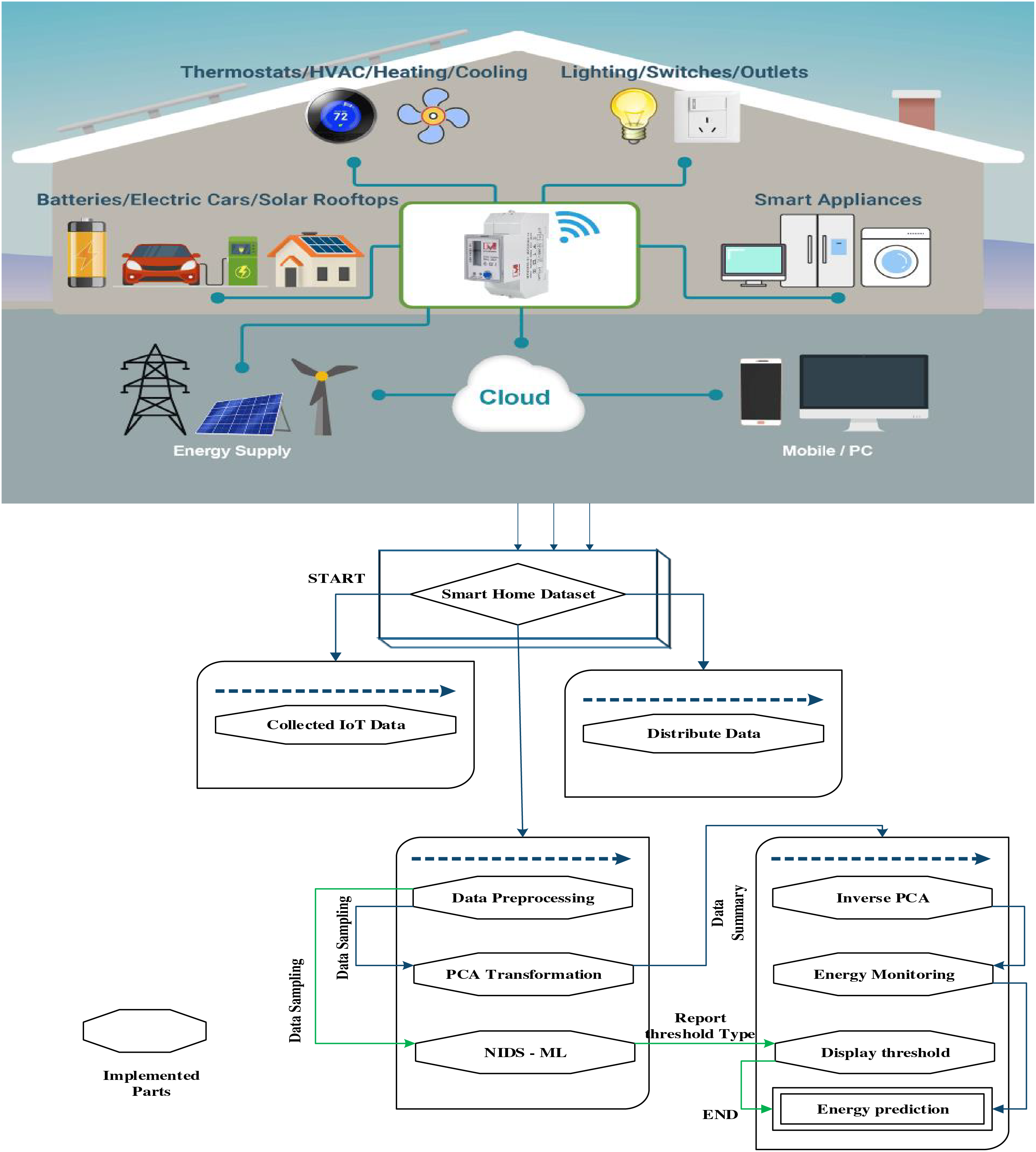
Figure 1: Proposed flowchart model

ADASYN

ADASYN solves the problems caused by datasets with an imbalance of classes using a sophisticated method. To address the underrepresentation of the minority class in certain feature space areas, ADASYN generates synthetic samples for that class. By improving the minority class’s representation while maintaining the majority class’s distribution, this strategy improves the model’s performance. For binary classification tasks, our method used an upgraded cascaded ADASYN algorithm twice; for multiclass classification tasks, it was applied nine times. By keeping the dataset balanced throughout, this method improved model training in both binary and multi-class situations by successfully addressing class imbalance.

Consider the samples from the minority class as Xi, and the k-nearest neighbors of Xi as N(Xi, k). Eq. (2) defines the total number of synthetic samples to be generated for each minority case, denoted as n_i.

nt=NMaf−NMtnNMin⋅(1−Ntk)(1)

In this context, NMaj  and NMin  show the disparity between the minority and majority groups by representing their sample numbers, accordingly. When detecting minority examples near decision boundaries, synthetic samples are typically created to enhance model performance. Ni is the total amount of minority class samples that lie inside the radius given by the k-nearest neighbors. The following formula, as shown in Eq. (2), is used to produce synthetic samples for each minority case Xi.

Xsym =Xt+γ⋅(Xf−Xt)(2)

where Xsyn, Xi are the minority sample, γ is a random integer between 0 and 1, and Xj is a neighbor chosen at random from the k-nearest neighbors of Xi; this guarantees that the synthetic sample is produced along the line segment between Xi and Xj. More specifically, 25,979 variables were found to be inaccurate or missing as a consequence of using wireless data collection. The question mark (?) appears in place of numbers in certain data sets. There should be no disrespect for the improper inclusion of missing values in the dataset. In addition, for the power load measurements from the previous day, the non-numerical values were replaced with the mean of the appropriate variables. The dataset was finally resampled hourly, with a single representative value for every hour derived from the aggregate of meter readings taken at minute intervals. A sanitized dataset was generated using the “fillna()” Python function.

3.3 Removing Outliers Using Z-Score

Extreme outliers in the sample were identified and removed using the Z-score. Every feature in the DataFrame has its z-score determined using the z-score function in SciPy. Stats module. Z-scores show the standard deviations from the mean of each data point. Any data point having a z-score higher than 6 in any characteristic was deemed an outlier and deleted, according to a threshold of 6. The dataset was kept clean and free of severe outliers by using this procedure for both binary and multi-class classification.

To further identify and remove outliers, the LOF approach was used after the z-score. In datasets where the density distribution is not uniform, LOF excels in locating data points with much lower density than their neighbors. We anticipated 10% of the data to be outliers; therefore, we designed the LOF using n_neighbors set to 20 with contamination set to 0.1. Samples were categorized as either outliers (−1) or inliers (1) after the LOF model was fitted. A cleaner dataset was obtained for further analysis by retaining just the inlier samples. Both the binary and multi-class classification models’ performance and reliability were improved by this dual approach to outlier reduction.

3.4 Feature Correlational Analysis

One statistical method for investigating possible connections between many variables is correlational analysis. Using the Python Pandas library, we analyzed the energy use information for correlations between variables. There is general agreement that the aforementioned process is a leading approach to evaluating correlations. The approach used in this research involves finding the correlations between each pair of variables or characteristics in the dataset. To measure the level of interaction between two columns or parameters, the procedure creates a linear connection between the dataset’s variables and calculates the correlation coefficient. On a unitary scale, the coefficient is shown to have values between one and one and a half. When the value of a parameter is 1, it means that the parameter is completely correlated with itself, showing a strong positive association. On the other hand, a correlation value close to 0 indicates a weaker link. But the fact that there is a unity number, regardless of its polarity, shows that there is more. The global active power variable is where most of the forecast effort is concentrated. Voltage is shown to have a negative association based on the investigation of the correlation among these measures and other factors. The global active power is highly correlated with the individual sub-meters.

3.5 XAI Integration

Our proposed technique integrates XAI and has three essential parts to provide a comprehensive understanding of the decision-making processes used by energy demand forecasting algorithms for smart home users. The three primary parts that make up the framework are:

•   An interface that promotes teamwork and gives users explanations that put people’s wants and needs first; a model for making predictions and forecasts; and a generator for reasoning and explanation.

To forecast and estimate future energy needs, the main component makes use of a pre-trained ML model. The study’s estimations are based on preprocessed data collected from certain appliances. The next part of the research will examine the variables that really matter when making a choice and will provide reasons for the expected outcome, which will be about the predicted energy use for the next week in particular. In addition, our collaborative interface will provide and showcase explanations that prioritize human perspectives, with the goal of helping people understand the reasoning behind certain actions. The forecasting model, the first part of our system, consists of two Long Short-Term Memory (LSTM) layers (or Gradient Boosting) followed by one fully connected layer.

Smart Metering Using SHAP

Any machine learning model’s output may be explained using SHAP, a game-theoretic technique. When it comes to smart meters, SHAP can provide light on how various input properties impact a model’s energy consumption forecast and other smart grid-related metrics. Smart metering relies on complicated machine learning models, and this may make such models more understandable and trustworthy. Envision a smart meter design that can anticipate energy needs by taking into account variables such as temperature, time of day, appliance use, and past data. SHAP may break out the impact of each component on the forecast. It may reveal, for instance, that the model’s energy consumption predictions are quite sensitive to temperature and time of day (peak hours). Customers may use this data to better understand their energy use trends, and demand response programs can benefit from it as well.

3.6 Home Energy Management via Q-Learning

Among the primary ML methods for making the best possible decisions in a non-deterministic setting is RL. Fig. 2 shows how an agent learns what to do in response to changes in its environment and then applies that knowledge to future interactions. Afterwards, the agent receives a reward from the environment, which includes the updated state of the environment. The agent keeps learning until it gets the most out of its surroundings in terms of cumulative rewards. One definition of an agent’s policy is the way it behaves in a given state; an agent’s main objective is to find the policy that maximizes reward. In this research, we work under the assumption that the setting is defined through a Markov decision process. This means that as an agent transitions states, it just takes into account their current state and the action they have chosen in that state, without taking into account all of their prior states or actions.

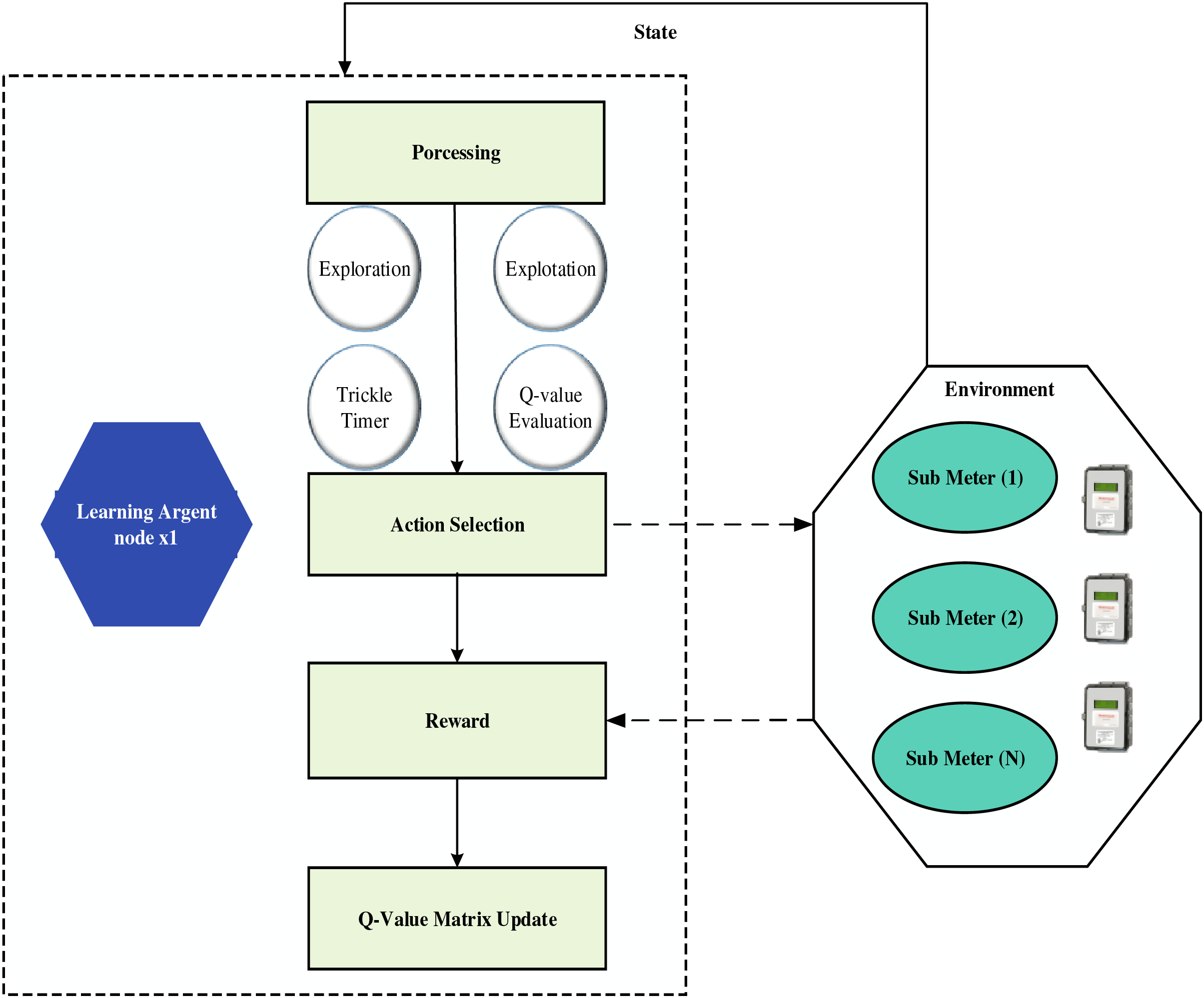
Figure 2: Q-learning for home energy management in smart grid

One of the RL strategies that stands out for finding the best policy v* in a decision-making situation is Q-learning. Applying the following Bellman equation, the standard procedure for Q-learning is to determine the Q-value Q(st, at) for a given state st and action at at a certain time t, and then to update the Q-value to maximize the total rewards:

QV∗∗(st,at)=r(st,at)+γmaxQ(st+1,at+1)(3)

The ideal Q-value, as shown in Eq. (3), is dependent on the optimum policy v^*Qv∗∗(st,at) becomes what is known as the greatest discounted future reward γ max plus the current reward r(st, at) Q(st+1,at+1) where γ∈[0,1] stands for a discounting element that clarifies how current and future benefits compare. The agent’s emphasis on the current reward increases as the factor of deduction γ drops, leading to short-sightedness. Nevertheless, the agent might grow more farsighted by focusing on the future payoff with a greater γ. The operator of the system may adjust the value of γ using Q-learning to strike a balance between immediate and future benefits, which is given in Fig. 2.

3.7 Socio-Economic Factors

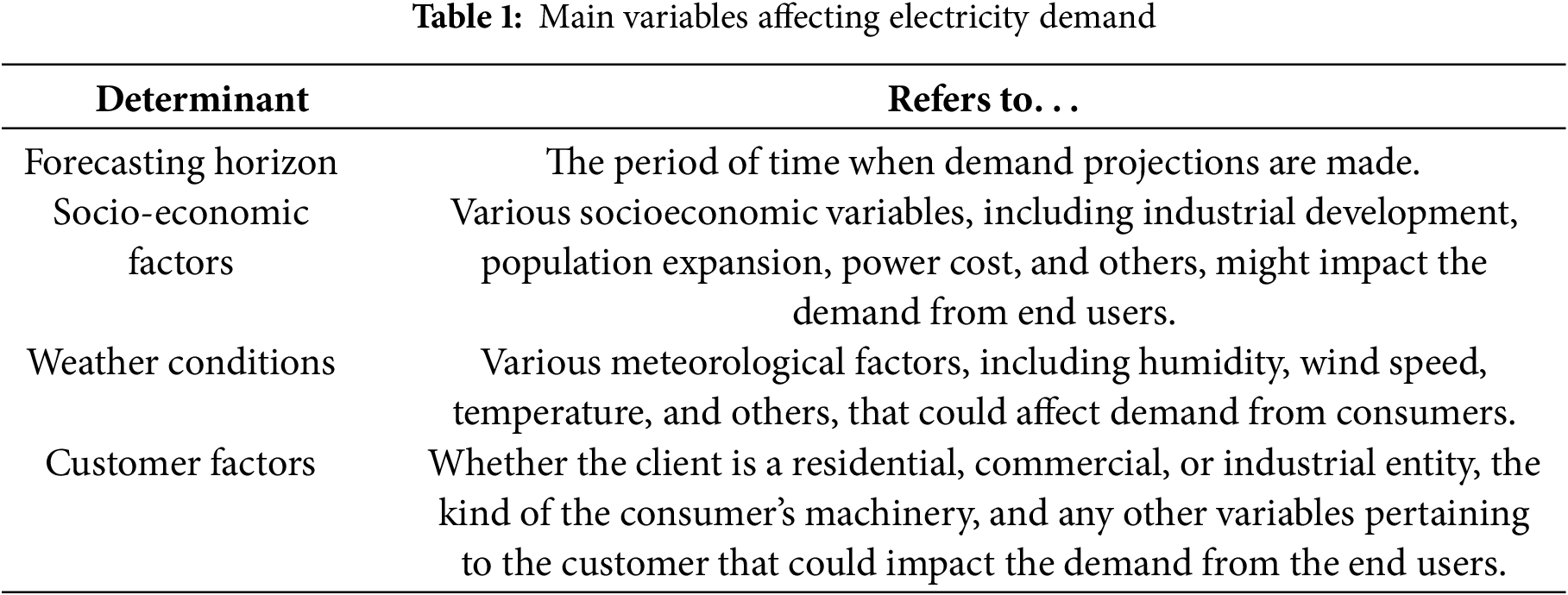
A number of socio-economic variables, such as GDP, the cost of power, and industrial growth, have a substantial impact on the change in demand. Economic considerations do, in fact, have a significant influence on both medium- and short-term demand estimates, as was shown in the preceding section. As an example, it is certain that energy consumption will rise as a result of industrial growth. The situation with population increase will be the same. This suggests that energy consumption rises in tandem with industrialization and population increase. A country’s economic activity may be captured by looking at its GDP. A larger GDP means more products and services produced, which means a better quality of living and more energy-intensive lifestyle patterns in the country. Because it influences demand as well, cost is another economic consideration. For instance, it’s common for people to use more power than they need if the price of electricity drops.

3.8 Weather Conditions

Demand forecasting makes use of a number of weather factors, including humidity, temperature, and wind speed, among others. Many scholars are interested in how the weather affects demand forecasts. Extreme heat waves in the summer put a strain on the power system. Actually, the electrical grid becomes more saturated during a heat wave, which impacts usage. One can use electricity, gas, timber, etc., to combat cold waves, while one can only use electricity to combat heat waves. So, most of the cooling equipment that people use nowadays is electrically driven. Therefore, heat waves cause greater strain on electrical cables and increased energy consumption.

It is worth mentioning that nations with cooler climates often have a smaller rise in consumption during heat waves. The reason is that, in cooler nations, air conditioning units are not installed as often. However, these colder nations are now experiencing heat waves that were not present before climate change, causing various issues due to their unpreparedness. As a result, these nations are implementing new policies, such as increasing the use of cooling equipment.

Humidity, on the other hand, makes the heat seem even more oppressive, particularly in the summer and after a rainstorm. Because of this, power use goes up on hot, muggy summer days. Also, keep in mind that power usage is often greater in coastal regions, like the Mediterranean area of Spain. Houses in this region often contain more electrical devices than those in other locations, and the high humidity from being so close to the sea also plays a role [10].

The speed of the wind also has an effect on power usage. When the wind is blowing, it makes people feel colder than they really are, so they need to turn up the heat, which in turn increases power consumption. But it’s also worth mentioning that wind power is a major renewable energy source. Put simply, the presence of wind causes an increase in power usage while simultaneously lowering its price. This is due to the fact that, as mentioned earlier, the power price is often set by combining several energy sources, ranging from the most affordable (renewables, wind, as well as nuclear) to the most costly (thermal, combined cycle).

Wind speed, humidity, and temperature all have an impact on electrical consumption. To reduce operational expenses, power demand forecast systems primarily employ temperature and humidity as meteorological factors. Nevertheless, other elements, such as clouds, are also influential. For instance, when clouds block the sun’s rays throughout the day, temperatures tend to decrease, and power usage increases.

3.9 Customer Factors

Other customer variables pertaining to power consumption (features of the consumer’s electrical equipment) and the kind of customer (residential, commercial, or industrial) may also impact demand. The reason is that there is a wide range in the kinds and sizes of equipment used by the residential, commercial, and industrial clients of most energy providers. The load curves for these various customer groups are not the same, yet there are some commonalities between commercial and industrial clients. Table 1 shows the main variables affecting electricity demand.

The state-action table, also known as the Q-value table, is updated whenever a certain state and action pair is entered at time t, with the result being Q(st,at). Whenever time t rolls around, the agent consults the Q-value table to choose what to do next. The Bellman equation is then used to update the Q-value associated with the chosen action and state:

Q(st,at)←(1−θ)Q(st,at)+θ[r(st,at)+γmaxQ(st+1,at+1)](4)

In Eq. (4), θ∈[0,1] depicts the pace of learning that decides how much the new Q-value takes precedence over the previous one. The agent does not learn anything and relies only on its previous Q-value at θ = 0, since it does not engage in exploration throughout the Q-learning process. On the other hand, when θ = 1, the agent doesn’t exploit anything; it just changes its Q-value based on the current reward and the maximum discounted future benefit. Just as when choosing γ, the system operator may find the balance among exploration and exploitation by adjusting the value of θ within the range of [0, 1]. Ultimately, the agent will achieve the optimum policy v* with the highest Q-value by iteratively updating Q(st,at) using Eq. (5), causing the Q-value to get greater:

v∗=arg maxQ(st,at)(5)

Applying the aforementioned Q-learning method to a single appliance (such as an air conditioner, washing machine, or ESS) in a smart home using a PV system and an ESS allows for the calculation of the optimal operation schedule of these appliances, which in turn reduces the consumer’s electricity bill while still meeting their preferred appliance planning and comfort levels. The next three parts provide a comprehensive example of the proposed Q-learning approach’s state, action, and reward.

3.10 State Space

Our scenario involves running the suggested Q-learning algorithm for 24 h with a 1-h scheduling resolution. For ∀t=1,…,24. Here, we can see the state regions of the washing machine (WM), the air conditioner (AC), and the energy storage system (ESS), in that order:

SWM={EtWM},SAC={EtAC},SESS={SOEtESS},(6)

where the states, EtWM,EtAC and SOEtESS stand for the ESS’s SOE, WM’s, and AC’s energy consumption at time t, respectively.

3.11 Action Space

As described in Section SHAP Result, the current condition of the agent and its surroundings determines the best course of action for each appliance. The following visualizes the WM, AC, along with ESS action spaces:

𝒜WM={On,Off},𝒜AC={0,ΔEAC,2ΔEAC,…,8ΔEAC,9ΔEAC},𝒜ESS={−4ΔEESS,−3ΔEESS,−2ΔEESS,−1ΔEESS,0,1ΔEESS,2ΔEESS,3ΔEESS,4ΔEESS}.(7)

3.12 Reward

Each appliance agent’s reward function is defined as the total of the negative electric cost, with negative displeasure cost linked to the consumer’s chosen comfort and the features of the appliance’s functioning. The HEMS includes a comprehensive reward rTotal 

rTotal =rtWM+rtAC+rtESS.(8)

In Eq. (8), the three reward functions, rtWM,rtAC, and rtESS seek to assess the HEMS efficiency by looking at three key metrics: (i) the power consumption and customer dissatisfaction with the WM’s operation, (ii) the power consumption and consumer discomfort with the AC’s temperature control, and (iii) the power consumption and energy waste caused by the ESS’s overcharging or undercharging.

To begin, the WM agent’s reward function is defined as

rtWM ={−[πtEtWM +δ¯(ωspref −t)], if t<ωspref ,−[πtEtWM +δ(t−ωfpref )], if t>ωfpref −πtEtWM , otherwise,(9)

where ωspref  and ωfpref  are the times that consumers like the WM to begin and end their workday, respectively, while δ and δ are the penalties for beginning and ending operations earlier and later, respectively, in comparison to the intervals that consumers desire. The WM agent adds a negative displeasure cost to the reward function if the WM energy usage is scheduled before ωspref  or after ωfpref ; Otherwise, a negative electric cost is the sole thing included in the reward function.

The AC agent’s reward function is defined as

rtAC={−[πtEtAC+κ(Tmin−Ttin)],if Ttin<Tmin−[πtEtAC+κ(Ttin−Tmax)],if Ttin>Tmax−πtEtAC,otherwise(10)

in which, κ represents the penalization for the customer’s temperature discomfort. Dissatisfaction cost is the amount by which actual temperatures deviate from the ideal range for a certain customer Ttin from, Tmln and Tmax only when it has a negative sign is it seen as the prize. TtLn deviates from the range of [Tmin,Tmax].

Lastly, a negative electric cost and a negative energy underutilization cost make up the incentive function for the ESS agent:

rtESS={−[πtEtESS+τ¯(SOEt−SOEmax)],if SOEt>SOEmax−[πtEtESS+τ_(SOEmin−SOEt)],if SOEt<SOEmin−πtEtESS,otherwise,(11)

where τ¯ and τ_ are overcharging and undercharging penalties of ESS, respectively. During the underutilization stage of the ESS, energy underutilization happens when the SOE falls below SOEmin (undercharging) or exceeds SOEmax (overcharging). This phrase is seen as a reward, coupled with the electric cost.

4  Results and Discussion

The effectiveness of our prediction approach in predicting home load performance is the main subject of this article’s thorough investigation of the experimental results. A dataset that has been gathered specifically for this study is used to perform the evaluation. The estimated values for the dataset on household energy use.

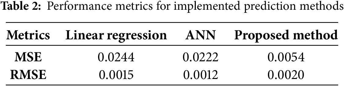
After importing the original dataset, features or parameters generated from time-series information were obtained. Based on the time-series data, we conducted the evaluation to determine the relative value of each characteristic. Resampling was performed on the dataset using time-series characteristics that show a strong statistical correlation. After that, three separate methods—MLR, linear regression, along with gradient boosting regressor—were used to train the data model from the dataset that had undergone extensive data cleaning as well as resampling processes. A total of 80% of the data was used for training purposes, with the remaining 20% serving as the evaluation dataset. Evaluation of the techniques using performance metrics, such as root mean squared error (RMSE), mean squared error (MSE), and mean absolute error (MAE), led to the adoption of the loss function. To measure the discrepancies between each anticipated value and its corresponding observed value, the root mean square error (RMSE) is used. Creating models that include both independent and dependent variables is within the range of possibility in time-series data analysis. The primary goal of these models is to provide a linear equation that faithfully depicts the underlying relationship between these variables. According to the hypothesis, x and y are two independent variables whose values are linearly related; in other words, y’s value depends on x’s value.

To test the dependent variable’s predictive power, a regression-based model uses a variety of independent variables during training. Many people refer to the concept being discussed as the model of MLR. Submetering_1, submetering_2, and submetering_3 are the data variables that make up the dataset used to forecast residential energy use.

All the experimental data are shown in Table 2. We ran the MAE, MSE, and RMSE calculations. Computational analysis was performed on the predicted values produced by models that used MLR with a gradient-boosting regressor. The dataset was resampled to a one-hour temporal resolution to improve computing performance and speed up the production of findings. Applying both models to the same dataset reveals that the gradient-boosting regressor approach outperforms MLR in terms of accuracy.

Gathering thorough data from numerous sources that might affect a home’s energy use is the first step in properly predicting and evaluating patterns of energy use and determining the causes of this consumption. The datasets have been structured and pre-processed to make ML model training more effective. Using sophisticated black box models in a training approach is the focus of the project. We use SHAP, an interpretable AI approach, to better understand the factors that impact household energy usage. The underlying causes of energy consumption may be more easily identified with the use of this technique. Given these issues, it’s critical to help different groups of people gain influence so that policies may be made that put an emphasis on making the most efficient use of energy.

SHAP Result

An important characteristic is one that has a significant effect on the target feature, in this case, electrical load. With such a high relevance score, the feature clearly has a significant impact on the desired function. The feature’s strong impact indicates its significant relevance to the target. Modifying these important elements may have a significant effect on the objective. Features were deemed to have little effect if their significance value was low. The target was unaffected or very slightly affected by these properties if they were deleted. Reducing computing complexity and improving simulation time are both achieved by removing unnecessary elements, which is shown in Fig. 3.

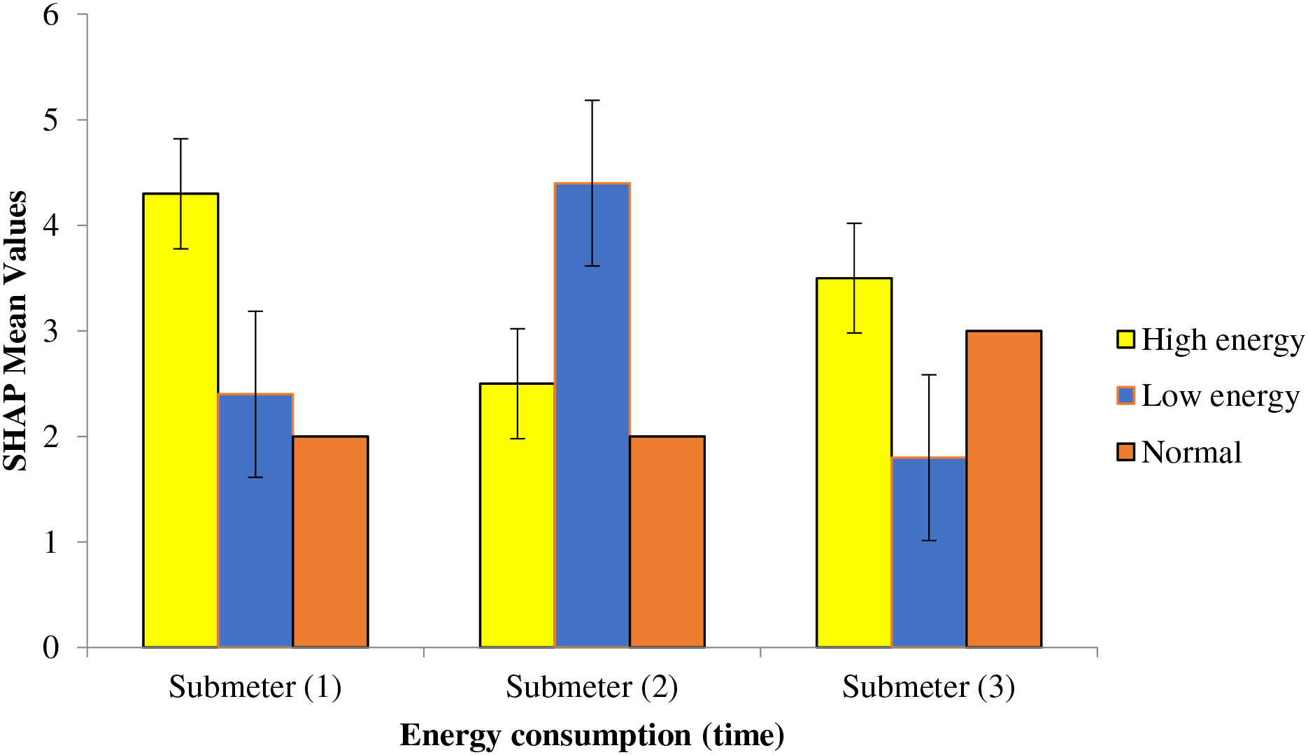
Figure 3: Smart metering (terminal access) using SHAP means values analysis

In particular, the graphic shows how various parts of the home utilize energy compared to one another. Our graphic’s primary objective is to show how different parts of the home have historically contributed to the overall energy use. Evidence from the visualization analysis points to the Sub_metering_3 variable having a substantial impact on the overall determination of energy consumption. The term “Sub_metering_3” describes the process of measuring and keeping tabs on the power use of certain components inside a bigger system.

Two of the most important equipment in every home are the water heater and the air conditioner. The most significant consequence was the beginning of the Sub_metering_3 contribution’s impacts. Additional features’ long-term effects are also shown in the supplied picture. Members of the family should become more aware of their energy use habits after reading these explanations. The use of the reasoning processes discussed earlier may also lead to AI models being trustworthy and transparent. A more thorough examination of the variables influencing global active power usage may be achieved by exchanging internal elements like Sub_metering_1 and Sub_metering_2, along with Sub_metering_3 with external factors like weather, pressure, cloud cover, along with user behavior, or vice versa. The objective is to find out how important and correlated certain aspects are by giving equal technical attention to internal and external factors. Whether it’s swapping out internal elements for external ones or the other way around, this method improves prediction transparency and helps with ethical AI modeling. Improved forecast accuracy and interpretability, as well as confidence in the model’s results, might result from a thorough understanding of the complex relationship between the two sets of variables. By standardizing the analysis and incorporation of these aspects, the study develops a complete and more trustworthy model for smart grid power consumption predictions.

5  Conclusion

Building and testing a home power load prediction mechanism was the focus of the current study. To accomplish this goal using ML techniques, the LSTM, XAI, and Q-learning frameworks were proposed. Predictive models that use feature extraction and related feature selection methods show a considerable reduction in computational time. Building a high-quality forecasting system is made much easier with the use of training data, which considerably increases the system’s efficiency and sharpens the accuracy of forecasts. A data resampling frequency of one hour yields the best results. The decreased RMSE achieved during training proves that the proposed method shows greater performance over ANN and Linear Regression. Nevertheless, it is essential to note that the proposed model is used together to achieve a balanced combination of speed and accuracy. A deeper dive into the link between ML and XAI as they pertain to sustainable smart city concepts is underway in this study. Applying SHAP methods to improve the interpretability of ML models within the framework of sustainable smart cities is our primary area of interest. This article provides a thorough review of ongoing research that aims to understand the challenges of creating an open and user-friendly system that can foretell and estimate smart home energy use. A new approach to explanation generation has been proposed, merging the approaches of Shapley Additive Explanations and LIME. The objective of this method is to provide explanations that are easy to understand to improve the understanding of predictions made by an LSTM-based forecasting model. An idea has been put out there that might help us better understand the unique needs of energy users if we combine a user-centered prototyping approach with various explanatory graphics. To better understand the dynamics of energy use and to build more accurate and insightful prediction models for smart grid settings, it is crucial to be able to interchangeably use internal and external variables. The main objective of this approach is to derive key findings and collect requirements for building a human-centered, collaborative system that can predict energy use. The capacity to provide explanations for its predictions is highly valued by the system. There will be more openness, justice, and personal accountability for those using the system once it’s up and running. To improve openness, justice, and accountability for those using it, this study stresses the need to be able to provide explanations for its predictions. The purpose of this article is to encourage conversations on intelligent decision-making in the context of sustainable smart cities and to add to the current body of knowledge on many criterion decision-making issues, such as electricity forecast. The Abbreviation list is as follows in Table 3.

Acknowledgement: Not applicable.

Funding Statement: The authors received no specific funding for this study.

Author Contributions: Sheng Bi: Writing—review & editing, Writing—original draft, Visualization, Data curation. Jiayan Wang: Writing—review & editing, Writing—original draft, Methodology, Formal analysis, Data curation. Dong Su: Writing—review & editing, Writing—original draft, Supervision. Hui Lu: Writing—review & editing, Writing—original draft, Supervision, Methodology, Conceptualization, Formal analysis, Data curation. Yu Zhang: Writing—review & editing, Writing—original draft, Supervision, Methodology, Conceptualization, Formal analysis, Data curation. All authors reviewed the results and approved the final version of the manuscript.

Availability of Data and Materials: Data sharing will not be applicable.

Ethics Approval: Not applicable.

Conflicts of Interest: The authors declare no conflicts of interest to report regarding the present study.

References

1. Fouad M, Mali R, Lmouatassime A, Bousmah M. Machine learning and iot for smart grid. Int Arch Photogramm Remote Sens Spatial Inf Sci. 2020;XLIV–4/W3–2020:233–40. doi:10.5194/isprs-archives-xliv-4-w3-2020-233-2020. [Google Scholar] [CrossRef]

2. Kothai Andal C, Jayapal R. Intelligent power and cost management system in small-scale grid-associated PV-wind energy system using RNN-LSTM. SN Comput Sci. 2023;4(6):746. doi:10.1007/s42979-023-02182-5. [Google Scholar] [CrossRef]

3. Barja Martínez S. Energy management systems for smart homes and local energy communities based on optimization and artificial intelligence techniques. [Ph.D. thesis]. Barcelona, Spain: Universitat Polit`ecnica de Catalunya; 2023. doi:10.5821/dissertation-2117-402846. [Google Scholar] [CrossRef]

4. Zjavka L. Power quality statistical predictions based on differential, deep and probabilistic learning using off-grid and meteo data in 24-hour horizon. Int J Energy Res. 2022;46(8):10182–96. doi:10.1002/er.7431. [Google Scholar] [CrossRef]

5. Zhao N, Lv J, Gao Y, Tang J, Zhou F. Real-time pricing for smart grid with multiple energy coexistence on the user side. IET Renew Power Gener. 2024;18(13):2162–76. doi:10.1049/rpg2.13051. [Google Scholar] [CrossRef]

6. Soni P, Subhashini J. Optimizing power consumption in different climate zones through smart energy management: a smart grid approach. Wirel Pers Commun. 2023;131(4):2969–90. doi:10.1007/s11277-023-10591-1. [Google Scholar] [CrossRef]

7. Zhang Z, Liu H. Non-cooperative energy consumption scheduling for smart grid: an evolutionary game approach. In: Advances in natural computation, fuzzy systems and knowledge discovery. Cham, Switzerland: Springer International Publishing; 2021. p. 1265–71. doi:10.1007/978-3-030-70665-4_137. [Google Scholar] [CrossRef]

8. Rashid U. Optimizing efficiency of home energy management system in smart grid using genetic algorithm. Sukkur IBA J Emerg Technol. 2024;6(2):11–20. doi:10.30537/sjet.v6i2.1363. [Google Scholar] [CrossRef]

9. Zhang L, Zhu Y, Ren W, Wang Y, Choo KR, Xiong NN. An energy-efficient authentication scheme based on Chebyshev chaotic map for smart grid environments. IEEE Internet Things J. 2021;8(23):17120–30. doi:10.1109/JIOT.2021.3078175. [Google Scholar] [CrossRef]

10. Shen L, Wang F, Zhang M, Liu J, Liu G, Fan X. AIoT-empowered smart grid energy management with distributed control and non-intrusive load monitoring. In: 2023 IEEE/ACM 31st International Symposium on Quality of Service (IWQoS); 2023 Jun 19–21; Orlando, FL, USA. p. 1–10. doi:10.1109/IWQoS57198.2023.10188781. [Google Scholar] [CrossRef]

11. Roy C, Das DK. Performance enhancement of smart grid with demand side management program contemplating the effect of uncertainty of renewable energy sources. Smart Sci. 2023;11(4):702–27. doi:10.1080/23080477.2023.2244262. [Google Scholar] [CrossRef]

12. Hu C, An D. Electric energy trading mechanism of distributed electric vehicles in smart grid. In: 2023 38th Youth Academic Annual Conference of Chinese Association of Automation (YAC); 2023 Aug 27–29; Hefei, China. p. 45–50. doi:10.1109/YAC59482.2023.10401661. [Google Scholar] [CrossRef]

13. Janjua JI, Ahmad R, Abbas S, Mohammed AS, Khan MS, Daud A, et al. Enhancing smart grid electricity prediction with the fusion of intelligent modeling and XAI integration. Int J Adv Appl Sci. 2024;11(5):230–48. doi:10.21833/ijaas.2024.05.025. [Google Scholar] [CrossRef]

14. Mahmood D, Latif S, Anwar A, Jawad Hussain S, Jhanjhi NZ, Us Sama N, et al. Utilization of ICT and AI techniques in harnessing residential energy consumption for an energy-aware smart city: a review. Int J Adv Appl Sci. 2021;8(7):50–66. doi:10.21833/ijaas.2021.07.007. [Google Scholar] [CrossRef]

15. Kiliç SK, Özdemir K, Yavanoğlu U, Özdemir S. Enhancing smart grid efficiency through AI technologies. In: 2024 IEEE International Conference on Big Data (BigData); 2024 Dec 15–18; Washington, DC, USA. p. 7068–74. doi:10.1109/BigData62323.2024.10825117. [Google Scholar] [CrossRef]

16. Khan MA, Saleh AM, Waseem M, Ali Sajjad I. Artificial intelligence enabled demand response: prospects and challenges in smart grid environment. IEEE Access. 2022;11(1):1477–505. doi:10.1109/access.2022.3231444. [Google Scholar] [CrossRef]

17. Ali W, Ud Din I, Almogren A, Khan MY, Altameem A. PowerTrust: AI-based trustworthiness assessment in the Internet of grid things. IEEE Access. 2024;12:161884–96. doi:10.1109/access.2024.3487617. [Google Scholar] [CrossRef]

18. Darmawan RR, Wijaya JP, Nadia FA. AI-based energy consumptions predictions in smart grids. In: 2024 International Conference on Artificial Intelligence, Blockchain, Cloud Computing, and Data Analytics (ICoABCD); 2024 Aug 20–21; Bali, Indonesia. p. 303–8. doi:10.1109/ICoABCD63526.2024.10704359. [Google Scholar] [CrossRef]

19. Du W, Guo Y, Du J, Wei Y, Han D. Construction of smart management model for power grid user side based on artificial intelligence and power BD. In: Third International Conference on Electronics, Electrical and Information Engineering (ICEEIE 2023); 2023 Aug 11–13; Xiamen, China. p. 235–42. doi:10.1117/12.3009123. [Google Scholar] [CrossRef]