Coordinated Scheduling of Electric-Hydrogen-Heat Trigeneration System for Low-Carbon Building Based on Improved Reinforcement Learning

1  Introduction

In the face of increasingly severe global climate change, the low-carbon transformation of the construction industry, as a significant component of energy consumption and carbon dioxide emissions, has become the key to attaining sustainable development [1]. Constructing efficient and clean building energy systems to reduce carbon emissions has become the focus of interest in the industry [2]. In this context, the electricity-hydrogen-heat trigeneration (EHHT) system provides substantial technical support for the low-carbon transformation of building energy systems by virtue of its benefits of high energy utilization efficiency, low pollutant emissions, and diversified energy supply.

By combining diverse kinds of energy and supplementing with energy storage devices, EHHT systems can effectively enhance energy usage efficiency and minimize dependence on traditional fossil energy sources, hence lowering carbon emissions [3]. However, there are still significant hurdles to achieve coordinated and optimal scheduling of multiple energy sources within an EHHT system to fully leverage its energy-saving and emission-reduction potentials [4]. Dispatch optimization coordinates the regulation of multiple energy flows, such as electricity, heat, and gas, and energy storage equipment, with the objectives of economic efficiency, low carbon emissions, and reliability, to address the strong uncertainty and complex multi-energy coupling issues caused by the high proportion of renewable energy integration. Its core lies in establishing an optimization framework that encompasses energy hub models, multi-energy network constraints, and uncertainty handling methods (such as stochastic programming or reinforcement learning) and utilizing mixed-integer programming, intelligent algorithms, or distributed optimization for solutions.

Traditional optimization approaches are generally difficult to attain optimum outcomes when dealing with complicated systems, uncertainties, and nonlinear interactions [5]. For example, due to the dynamic changes in electricity price, load demand, renewable energy output and other factors, the operation optimization of EHHT systems needs to consider numerous constraints and uncertainties, making it difficult for traditional optimization methods to meet the actual needs in terms of computational efficiency and global optimization search capability [6]. In addition, these classic optimization approaches frequently involve the construction of precise system models, including equipment models, load models, energy pricing models, etc. [7]. Establishing an accurate model needs a great quantity of data and skill, and it is challenging to explain the uncertainties adequately in the system [8]. Even if the model is constructed, it is impossible to ensure the accuracy of the model, and the model mistake may contribute to the departure of the optimization outcomes [9]. Consequently, conventional optimization techniques frequently struggle to attain optimal outcomes in complicated EHHT system scheduling issues, necessitating the urgent development of a novel optimization approach to address these challenges.

As an intelligent optimization method, RL (Reinforcement Learning) provides a promising solution to the coordination and scheduling challenges of EHHT systems [10]. RL learns the optimal control strategy by interacting with the environment and possesses the ability of self-adaptation and dealing with complex problems [11]. It circumvents the reliance on exact system models and learns control strategies autonomously by interacting with the environment without the need for complex mathematical models [12]. The Deep Deterministic Policy Gradient (DDPG) algorithm is particularly suitable for the coordinated scheduling problem of EHHT systems, capable of dealing with continuous action spaces, and highly compatible with the control requirements of EHHT systems, and it has convergence and robustness [13]. Therefore, RL, especially the DDPG algorithm, provides a novel and effective solution for the coordinated scheduling of EHHT systems. Currently, demand response research has also been conducted under simple models [14]. As system complexity increases, traditional DDPG algorithms often suffer from slow convergence speeds and poor performance. Therefore, developing a novel DDPG algorithm for EHHT optimization scheduling will help improve energy efficiency, reduce operational and carbon dioxide emissions, and facilitate the low-carbon transformation of building energy systems.

The aim of this paper is to investigate a coordinated scheduling strategy for low-carbon building EHHT systems based on DDPG. The main contributions of this paper are:

•   An EHHT system model is built that takes into account various energy sources, such as heat, hydrogen, electricity, and energy storage devices. The corresponding Markov decision process is also designed, providing a foundation for the efficient scheduling of the EHHT system.

•   To optimize system operation, increase energy usage efficiency, reduce carbon emissions, and account for the effects of numerous uncertainty factors, a coordinated scheduling technique (I-DDPG) based on the improvement of DDPG is proposed for the EHHT system.

•   A theoretical foundation for the real implementation of EHHT systems in low-carbon buildings is provided by simulation studies that compare I-DDPG with the outdated DDPG approach and show significant improvements in system energy efficiency and operation cost.

2  System Model and Optimization Problem Setting

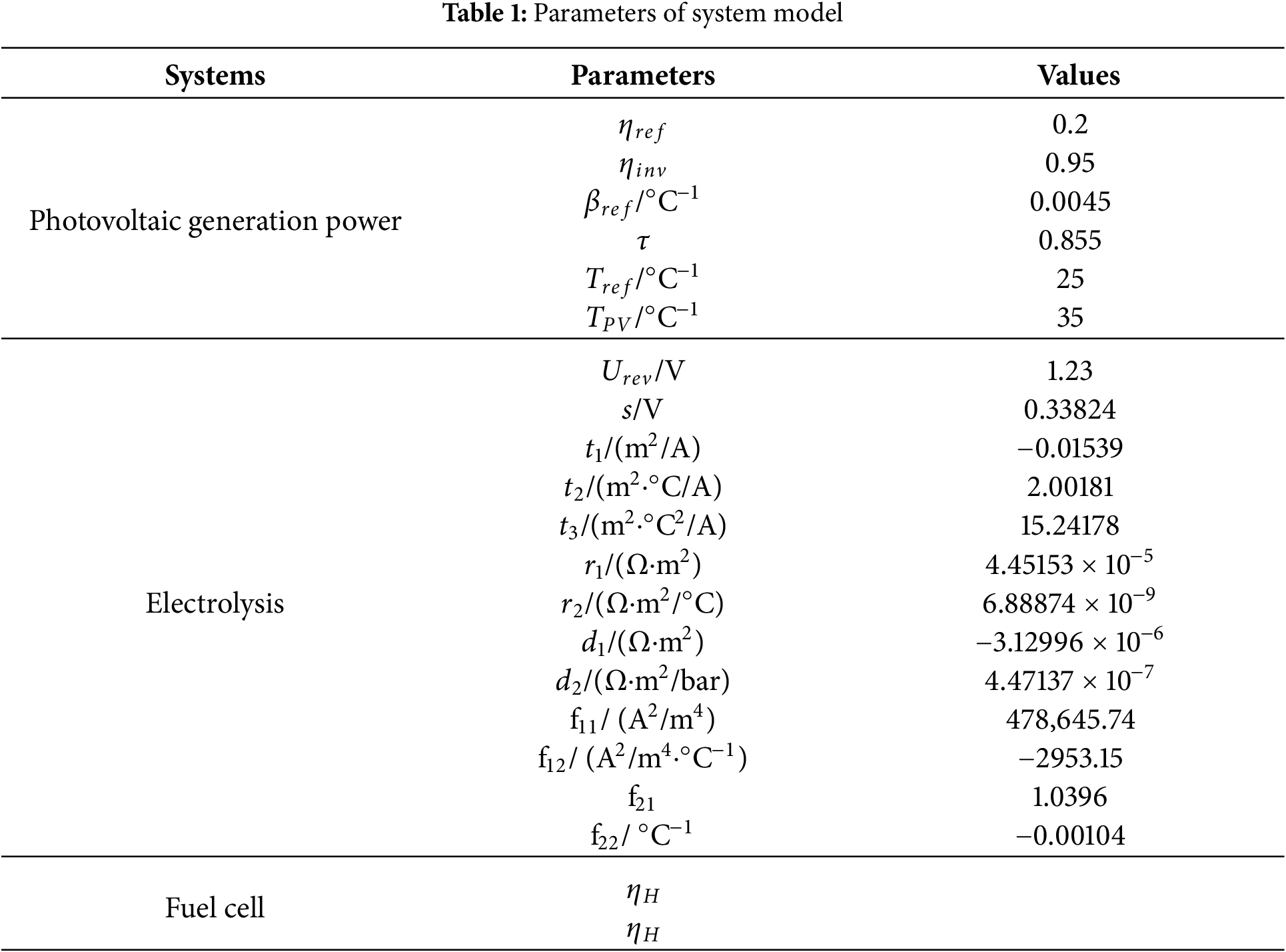
The flow of EHHT is shown in Fig. 1, which includes a photovoltaic (PV) power generation unit, an alkaline electrolytic water unit (AEW), a hydrogen storage unit (HST), a proton exchange membrane fuel cell unit (PEMFC), a heat pump unit (HP), and a thermal energy storage unit (TES). The PV is supplied to the building occupants while the excess power is used for the AEW, which is thus stored in the form of hydrogen energy. In the scenario where there is no PV at night, the stored hydrogen is used in the PEMFC to generate electricity, while the coupled heat pump recovers and refines the heat generated by the battery, which is stored by the HS for supplying to the users. The system parameters are shown in Table 1. In addition, all internal models used in this study have been validated in relevant studies.

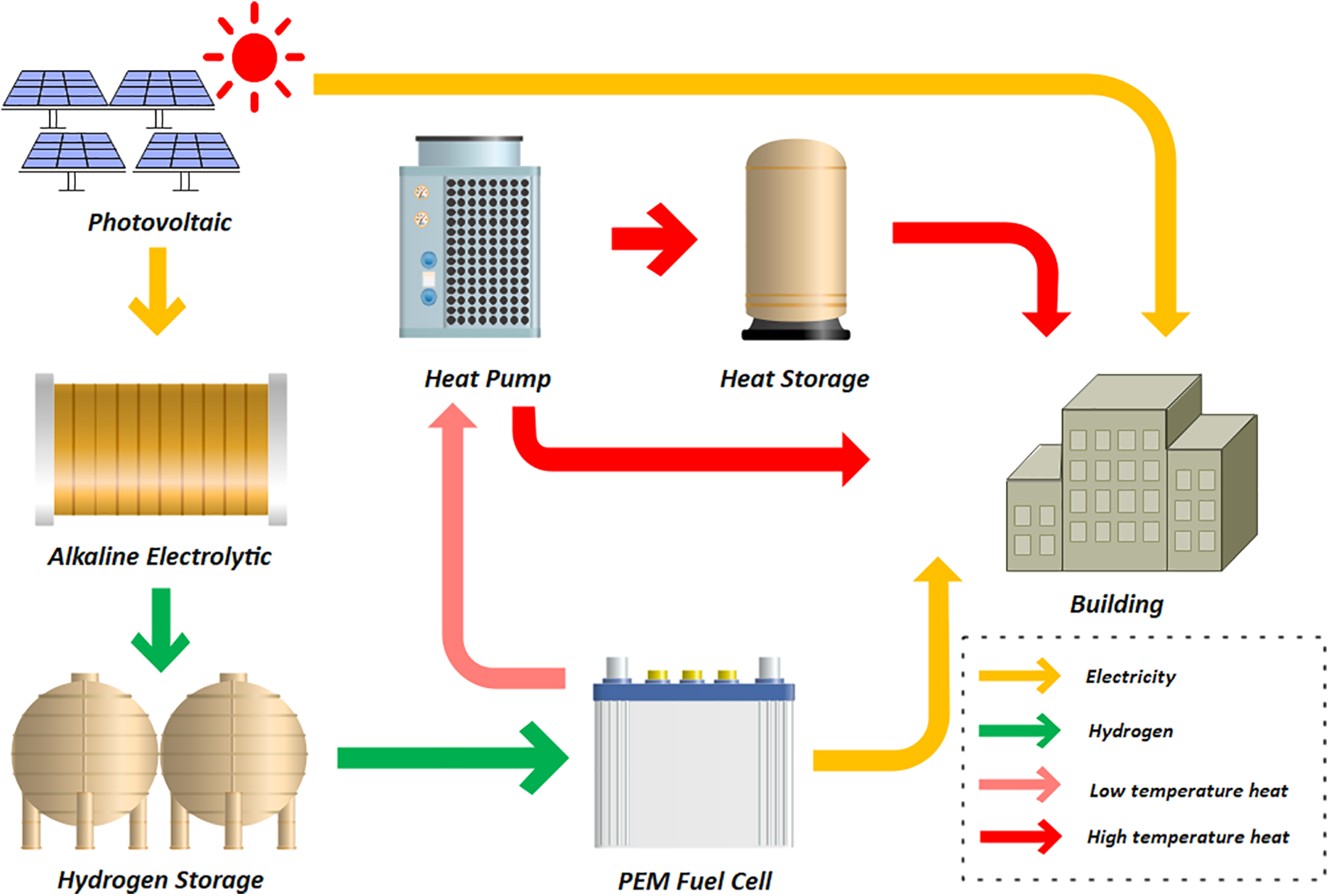
Figure 1: Processes of electric-hydrogen-heat trigeneration system for low-carbon building

2.1 Photovoltaic Generation Power Model

PV power generation model, refer to the study of Li et al. [15]. The calculation of PV power generation Pel is shown in Formula (1).

Pel=ηinvηPVτAPVNPVG(1)

where τ denotes optical efficiency, APV denotes PV area, G denotes radiation intensity, NPV denotes the number of PVs, and ηinv denotes the photovoltaic conversion efficiency. ηPV denotes the photovoltaic efficiency, calculated as shown in Formula (2).

ηPV=ηref[1−βref(TPV−Tref)](2)

where ηref denotes the reference efficiency, βref denotes the temperature reference factor, Tref denotes the reference temperature, and TPV denotes the effective PV temperature.

2.2 Electrolysis Model

The model of hydrogen production by electrolysis mainly consists of electrolysis voltage, hydrogen production and electrolysis power. The electrolysis voltage Ve is calculated as shown in Formula (3) [16].

Ve=Vr+[r1+d1+Te⋅r2+pe⋅d2]⋅ie+k⋅log⁡[(t1+t2Te+t3Te2)+1](3)

where Vr denotes the reversible potential, ie denotes the current density, ti and k denote the activation impedance, r and d denote the ohmic impedance factor, Te and pe denote the electrolysis temperature and electrolysis pressure, respectively.

Hydrogen yield nH2,production calculations are shown in Formulas (4) and (5):

nH2,production=Ne⋅ie⋅Ae⋅ηF2F(4)

ηF=(ie2f11+Te⋅f12+ie2)⋅(f21+Te⋅f22)(5)

where Ne denotes the number of electrolyzer, Ae denotes the area of electrolysis, ηF and F are the Faraday constant and Faraday efficiency, respectively.

Electrolytic power We can be expressed as the product of electrolytic voltage Ve, current density ie, number of electrolytic cells Ne and electrolytic area Ae, calculated as shown in Formula (6).

We=Ne⋅Ve⋅ie⋅Ae(6)

2.3 Hydrogen Storage Tank Model

The hydrogen storage tank is used as a daytime storage for hydrogen produced from PV electrolysis and supplied to the fuel cell at night to generate electricity. The formula for the pressure of the hydrogen storage tank as a function of time is shown in Formula (7) [17]:

TPt+1H=TPtH−ztnH2,tRTH2VH(7)

where TPiH and nH2,t denote the hydrogen storage tank pressure and hydrogen flow rate at a certain moment, TH and VH denote the hydrogen storage tank temperature and hydrogen volume, respectively. zt denotes the hydrogen compression factor, which is calculated as shown in Formula (8).

zt(TPt)=1+∑i=19ai(TrefTH)bi(TPt)ci(8)

2.4 Fuel Cell Model

Hydrogen consumption is the key variable when scheduling the fuel cell system in the EHHT system and is calculated as shown in Formula (9) [18].

nH2,consumption=Nfc⋅ifc⋅Afc2F(9)

where Nfc, Afc and ifc denote the number of cells, cell area, and cell current density, respectively. In addition, the fuel cell exotherm considered, the recoverable heat can be calculated by Formula (10).

Qfc=WfcηHηE(10)

where Qfc and Wfc denote the battery heat production and power generation, respectively, ηH and ηE denote the battery thermal efficiency and power generation efficiency, respectively.

2.5 Heat Pump Model

Heat pumps, as a system that can recover waste heat and further improve the quality, can be combined with fuel cells to provide higher temperature heat demand for buildings [19]. COP (coefficient of performance) as a key metric for evaluating heat pumps is calculated [20] as shown in Formula (11).

COP=h1−h2ΔTHP+h3ΔTHP2,15≤ΔTHP≤60(11)

where hi denotes the coefficient for calculating the COP, hi(i=1,2,3) take the values 6.81, 0.111, 0.00063, respectively. And ΔTHP denotes the difference between the lifting temperature and the reference temperature. The amount of heat that can be provided by the heat pump QHP is calculated as shown in Formula (12).

QHP=WHP⋅COP(12)

where WHP denotes the power consumption of the heat pump.

2.6 Thermal Energy Storage Model

Considering the uncertainty in the scheduling of heat demand in buildings, excess heat needs to be stored, hence the need for a thermal storage system. The key parameter of the thermal storage tank is quantified in terms of TESD (Thermal energy storage degree) which is calculated as shown in Formula (13) [21].

TESDk+1=TESDk−QTES,kHcΔT(13)

where QTES,k represents the heat exchange power of the thermal storage system. Positive and negative values of this variable indicate the exothermic and impulsive processes of the thermal storage system, respectively. Hc for the maximum heat storage tank heat storage capacity.

2.7 Optimization Problem Formulation

In the EHHT, the integration of the hydrogen storage tank with the thermal storage tank significantly enhances the flexibility of the system. Specifically, when the daytime PV power output exceeds the immediate demand, the system directs the excess power resources to the electrolyzer for hydrogen production, and stores the produced hydrogen in the hydrogen storage tank for use at nighttime. In view of this operation mechanism, the core of the dispatch optimization problem for the described EHHT is to rationally deploy the generation output power of the fuel cell, the power consumption power of the heat pump, and the electrolysis power of the electrolysis tank, with the aim of minimizing the operation cost of the system while maximizing the sustained and efficient operation capability of the system. Based on this objective, this study constructs a corresponding objective function system and sets a series of necessary constraints to ensure the scientifical and feasibility of the optimization process.

(1) Objective functions

J=min∑t=1T(λ1COM,t)+CT{COM,t=∑kOMkPk,tCT=λ2|HSDT−HSD0|+λ3|TPT−TP0|(14)

where k represents different devices, OMk corresponds to the unit operating cost of device k, and Pk,t denotes the power output of device k at time t. The coefficients (λ1, λ2 and λ3) are parameters to be calibrated to balance the operating cost of the system with the sustainable operating cost. The coefficients are parameters to be calibrated to balance the system operating expenses with the sustainable operating expenses and to ensure that they are harmonized on an order of magnitude. In addition, HSD0 and TP0 refer to the energy storage levels of the heat storage and hydrogen storage tanks at the beginning of the scheduling cycle, respectively, while HSDT and TPT correspond to the energy storage status of the two storage devices at the end of the scheduling cycle. The initial energy storage states of the heat storage tank and the hydrogen storage tank are set as follows:

HSD0=(HSDmax+HSDmin)⋅0.5(15)

TP0=(TPmax+TPmin)⋅0.5(16)

where HSDmax and HSDmin denote the upper and lower limits of the energy storage state of the thermal storage tank, respectively. TPmax and TPmin are the upper and lower limits of the energy storage state of the hydrogen storage tank, respectively.

(2) Balance and equipment constraints

Ensuring that a set of constraints is met during system operation is critical to maintaining the safety and stability of the system. These constraints cover the supply-demand balance between the EHHT and the users, the power output limits of the components within the EHHT, and the climbing power limits of the energy storage devices. In view of this, the following power balance constraints and equipment power constraints are set:

PE,tFC+PE,tPV=PE,tL+PE,tHP+PE,tEC(17)

PH,tFC+PH,tHP+PH,tTES=PH,tL(18)

PE,minFC≤PE,tFC≤PE,maxFC(19)

PE,minHP≤PE,tHP≤PE,maxHP(20)

PE,minEC≤PE,tEC≤PE,maxEC(21)

NminHST≤NFC,t≤NmaxHST(22)

NminHST≤NEH,t≤NmaxHST(23)

HSDmin≤HSDt≤HSDmax(24)

TPmin≤TPt≤TPmax(25)

Among them, Formulas (17) and (18) are the constraints of the set-up electric-heat supply-demand balance, Formulas (19)–(21) represent the constraints of the fuel cell output power, the electric power used by the heat pump, and the electrolysis power of the electrolysis tank, Formulas (22) and (23) are the constraints of the hydrogen flow rate of the hydrogen inlet and outlet of the hydrogen storage tank, and Formulas (24) and (25) are the constraints of the energy storage state of the heat storage tank and the hydrogen storage tank, respectively.

In the system optimization process, the core challenge stems from the inherent uncertainty of renewable energy sources and the complexity of the system model, which covers the phenomenon of multi-energy-flow coupling and source-load uncertainty, which significantly enhances the planning difficulty of the scheduling strategy. Traditional rule-based scheduling algorithms are highly dependent on the experience of experts, and their scheduling performance is often unsatisfactory in the face of unknown scenarios. In addition, both standard optimization algorithms and general-purpose reinforcement learning algorithms usually require the system state to be discretized or optimized in predefined scenarios, which leads to poor scheduling performance in real-world environments full of uncertainty. uncertainty problem encountered during the actual operation, thus overcoming the above limitations. In particular, the DDPG algorithm can deal with continuous state and action space directly, which significantly enhances the real-time response speed and operation efficiency of the system in complex and changing environments. The following section details how the DDPG algorithm can be utilized to address the multi-dimensional uncertainty challenges faced by EHHT.

3  Deep Deterministic Policy Gradients

3.1 Markov Decision Process

Markov Decision Process (MDP) provides a solid and stable theoretical framework for the field of reinforcement learning by accurately characterizing the dynamics of system-environment interaction. Specifically, it skillfully transforms complex scheduling optimization problems into sequential decision-making problems, i.e., dynamic decision-making and planning over continuous time series. A standard MDP usually consists of five core elements: state space, action space, state transfer probability matrix, reward function, and discount factor. Given that this paper adopts a reinforcement learning algorithm for prediction-free modeling, the MDP model constructed in this paper can be formulated as follows:

•   state space

In the Markov decision process model constructed in this paper, the key parameters of the system operation are comprehensively covered, specifically, the time variable, the electric load demand, the heat load demand, the storage level of the heat storage tanks, and the storage state of the hydrogen storage tanks. These state variables are expressed through the following mathematical formulas:

st=[t,PE,tL,PH,tL,PE,tPV, HSDt, TPt]T(26)

•   action space

The action space includes the power generated by the fuel cell, the power used by the heat pump, and the electrolysis power of the electrolyzer.

αt=[PE,tFC,PE,tHP,PE,tEC]T(27)

•   reward function

Within the reinforcement learning framework, the construction of the reward function is a crucial aspect that profoundly affects the overall effectiveness of the algorithm. Therefore, it is indispensable to ensure that the reward function is set appropriately. It is worth noting that even if the energy storage device is introduced as a regulating mechanism to mitigate the impact of instantaneous decisions, it is still difficult to ensure that the decisions made can strictly comply with the preset constraints at the early stage of training, as the algorithm is usually initialized with stochastic parameters at the initial stage. To address this challenge, this paper integrates an additional penalty term in the reward function, aiming to accelerate the convergence process and improve the performance of the algorithm, as well as to ensure that the decision-making process always stays within the constraint bounds. Based on the above considerations, the reward function designed in this paper is formulated as follows:

R={−rt,0<t<T−1−(rt+CT),t>=T−1rt=λ1COM,t+λ4Cout,tCout,t=μ1PH,tout+μ2PTP,tout+μ3PE,tout(28)

where the first term of the reward function is consistent with the objective function of the scheduling optimization problem COM,t and CT are given in Formula (14). Cout,t are additional penalties, in which thermal imbalance penalties, hydrogen storage tank pressure constraint penalties, and electrical imbalance penalties are PH,tout, PTP,tout and PE,tout, respectively, λ4, μ1, μ2 and μ3 are parameters to be adjusted to ensure that the algorithm can quickly and efficiently converge to an optimization strategy that satisfies all the constraints during the training process.

3.2 Improvement of Reinforcement Learning Algorithm

Within the framework of traditional DDPG algorithms, to enhance the exploration capability, Ornstein-Uhlenbeck (OU) noise is introduced as a key tool aimed at improving the algorithm’s exploration efficiency in the state space. Specifically, the mechanism superimposes OU noise on the actions outputted by the actor (Actor) network at each time step and subsequently utilizes the noise-laden actions to interact with the environment. In addition, by designing a decay strategy for the noise, the algorithm is able to achieve a dynamic balance between exploration and exploitation. However, the introduction of OU noise in the early stages of training may lead to a potential problem: even if certain actions perform well on their own, their actual effects may be weakened due to the interference of noise, which may cause the algorithm to miss the opportunity of accumulating these high-quality experiences.

In light of the above considerations, this paper proposes a multiple exploration mechanism that aims to optimize the initial learning phase of the algorithm to ensure that these potentially beneficial experiences can be captured and exploited earlier and more efficiently. The mechanism is initially designed to reduce the number of high-quality action experiences that are accidentally overlooked due to the addition of noise, thereby facilitating the algorithm to reach a more efficient and robust balance between exploration and exploitation. Fig. 2 details the specific steps of the algorithm optimization process. Specifically, while noise is introduced during the execution of an action, the original action (i.e., the action without added noise) and an adjusted action obtained by directly subtracting the corresponding noise value from the original action are preserved. To preserve the empirical information accumulated by the original algorithm, the experience gained from the noise-containing action’s interaction with the environment is set as an item that must be preserved. Subsequently, the other two actions (original action and adjustment action) were allowed to interact with the environment as well, and the set of action experiences with the highest reward value was selected from them. Next, this set of action experiences is compared with the experiences generated by the noise-containing action in terms of reward value: if the reward value is higher than the reward value corresponding to the noise-containing action, then this set of action experiences is stored in the experience buffer along with the original experiences; otherwise, only the original experiences are stored in the experience buffer alone.

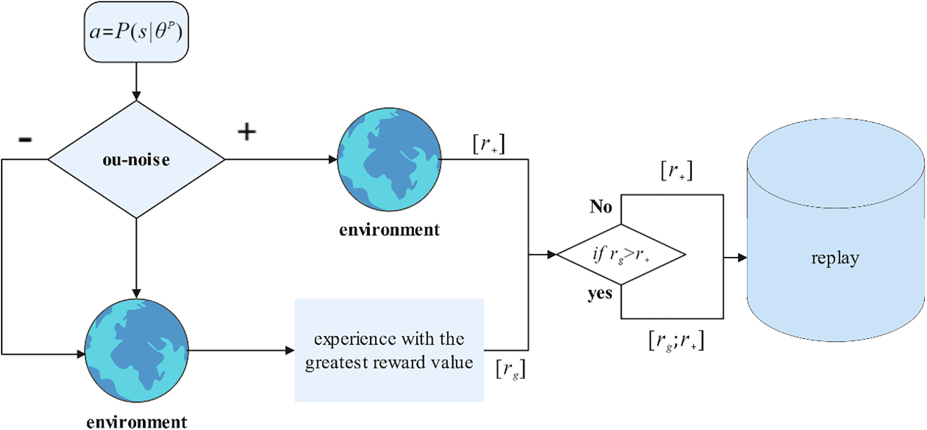
Figure 2: Operational process improved reinforcement learning algorithm

3.3 Algorithm Parameters and Network Initialization

In algorithm design, the selection of key parameters plays a crucial role in algorithm performance. For example, in the process of neural network training, if the learning rate is set too high, it may lead to the phenomenon of gradient explosion, thus hindering the effective updating of the network weights; on the contrary, a learning rate that is too low will make the learning process of the algorithm become sluggish and slow down the convergence speed, which in turn affects the final learning effect. Therefore, in the scheduling optimization process, reasonable parameter configuration constitutes an indispensable link. Table 2 [22] details the values of several key parameters in the scheduling optimization algorithm proposed in this paper.

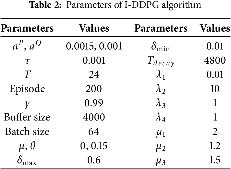
Fig. 3 shows in detail the network initialization architecture used by the algorithms in this study. Specifically, each network, i.e., P-network and Q-network, consists of an input layer, a hidden layer, and an output layer. In the hidden layer construction, FC represents the fully connected layer, which is responsible for achieving extensive connectivity between neurons, and LN represents the layer normalization layer, which aims to improve the training stability and convergence speed of the model. In addition, Relu and sigmoid functions are used as activation function layers, respectively, to introduce nonlinear properties to enhance the expressive power of the network.

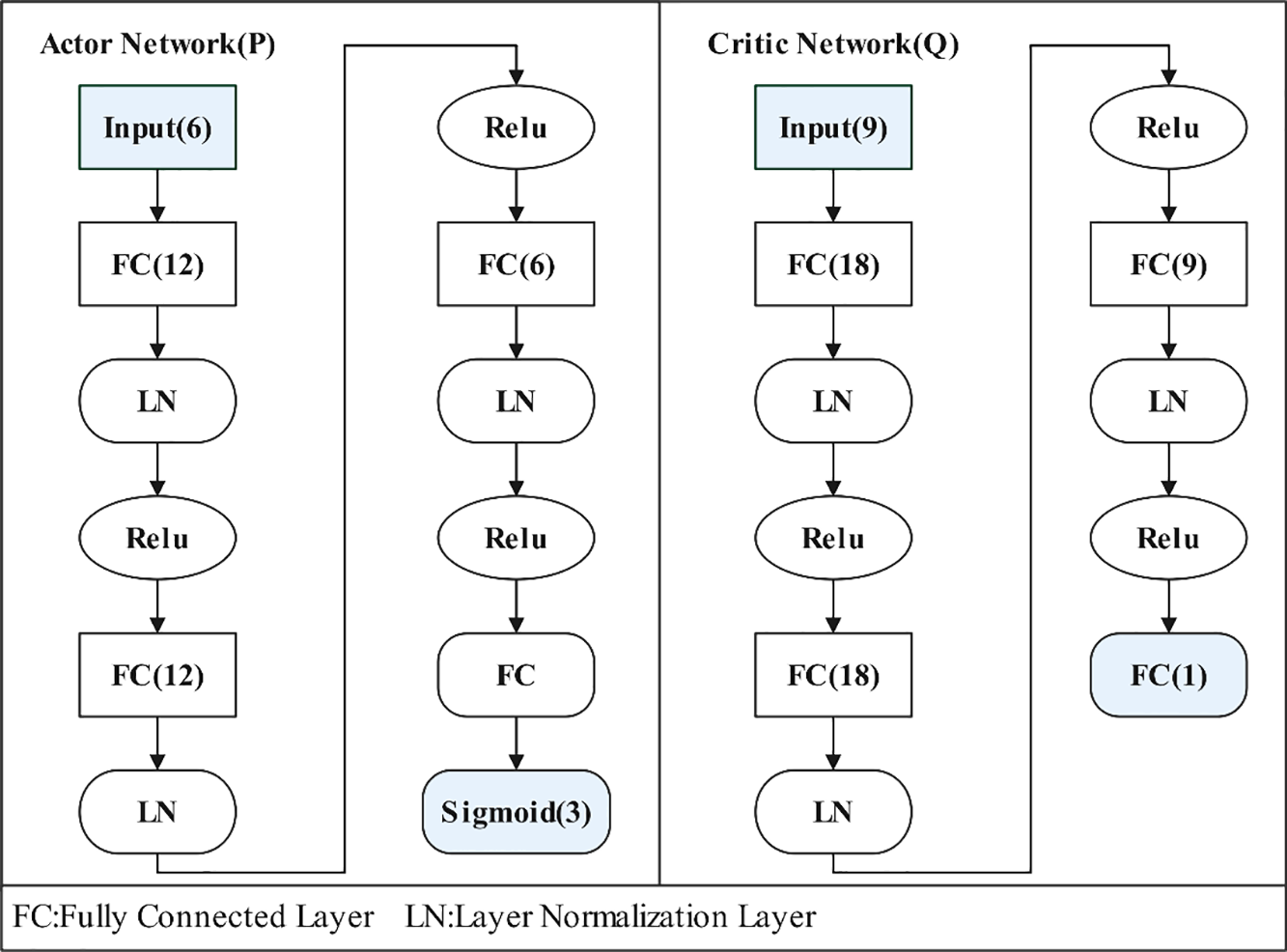
Figure 3: Network initialization structure of I-DDPG

As can be observed from the presentation in Fig. 3, the P-network is designed as a network structure with six input nodes and three output nodes. It is responsible for receiving state information from the environment and outputting the corresponding action strategies accordingly. In contrast, the Q network is configured as a structure containing 9 input nodes (corresponding to combinations of states and actions) and 1 output node, whose function is to receive state-action pairs as inputs and to output an assessment of the value of that state-action pair. Such a network design reflects the different functions and roles of the strategy network and the value network in reinforcement learning.

4  Results and Discussion

Initializes the scene, then analyzes the comparison results of a typical day scene, and finally compares the performance of the scheduling algorithm under random conditions.

4.1 Simulation Scene Initialization

To simulate the source-side and load-side uncertainties encountered in the actual operation of the EHHT, this study devised a methodology whereby a series of source-load scenarios are randomly generated based on a preset typical day scenario before each training iteration. Specifically, this process involves introducing a source-load fluctuation of no more than 30% into the typical scenarios as a baseline prior to the start of each training iteration to simulate the uncertainties that exist in the actual operating environment of the EHHT. The implementation of an optimal scheduling strategy in this uncertainty framework aims to enhance the robust performance of the algorithm in the face of uncertainty scenarios. The typical daily scenarios used in this study are illustrated in Fig. 4, which includes the electrical load (E), thermal load (H), PV power (PV), and ambient temperature (TE).

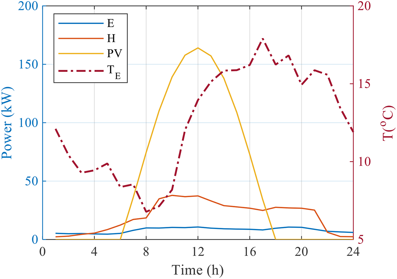
Figure 4: Variation diagram of the EHHT system in a typical day scene source load

4.2 Experimental Results and Analysis under Typical Day Scenarios

To ensure the rigor and reliability of the comparative analysis of the algorithms, this study preserved the source-load scenes and their accompanying noise data generated by the original algorithm in the training phase during the implementation of the optimal scheduling strategy for the established algorithm. In addition, the complete consistency of the network initialization parameters is ensured, i.e., the training process is re-run with the improved algorithm using the same training scenario with the same noisy dataset under the same network initialization configuration. This series of measures aims to ensure the reliability of the comparison experiments and the validity of the results so as to accurately assess the performance difference between before and after the algorithm improvement.

Fig. 5 visually presents a comparison of the convergence curves of I-DDPG and the original algorithm while keeping the same source-load scenario, noise characteristics, and network initialization parameter settings. During the initial exploration phase of the algorithm, both exhibit large negative reward values, reflecting the fact that the algorithm has not yet found an effective strategy in its initial attempts. As the training process progresses, I-DDPG continues to show a significant advantage over DDPG in terms of reward values, thanks to its designed mechanism of storing multiple sets of excellent experiences. Specifically, I-DDPG begins to converge gradually at about 140 training rounds, although there are still slight fluctuations due to noise disturbances, while the DDPG algorithm delays until about 160 rounds before it begins to converge. In terms of convergence speed, I-DDPG achieves a 12.5% improvement over the original algorithm. To further refine the analysis, the inset in Fig. 5 partially zooms in on the reward values of the last 20 training rounds, thus clearly demonstrating the difference in convergence values between the two. The results indicate that the average reward value of the DDPG algorithm in the last 20 rounds is −3.0498, while that of I-DDPG improves to −2.3542. At the level of converged mean value, I-DDPG achieves a 22.8% improvement compared to the DDPG algorithm. This significant improvement not only validates the reasonableness of the proposed improvements in this paper but also highlights the advantages of I-DDPG in improving training efficiency and performance.

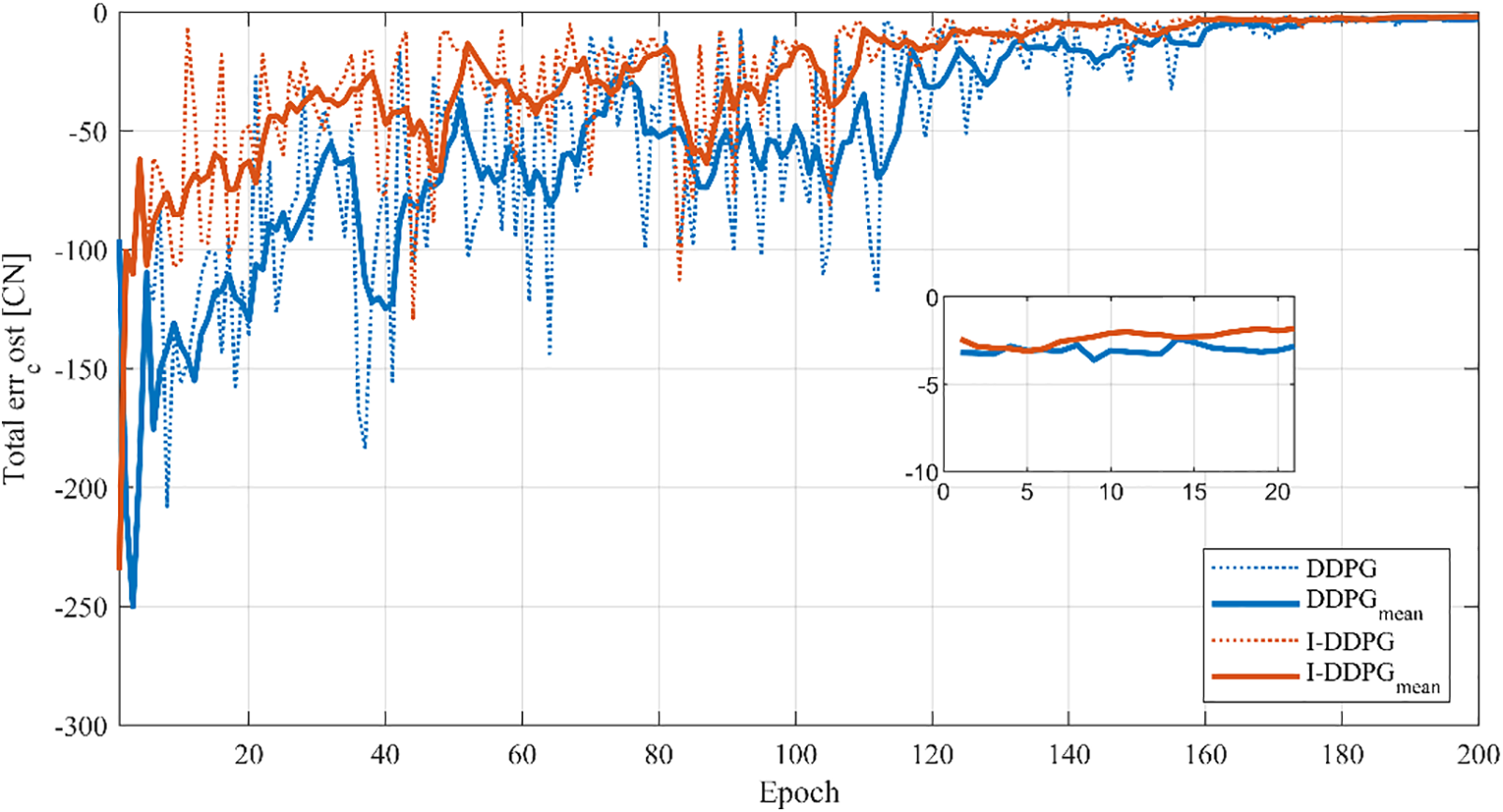
Figure 5: Comparison of different algorithm convergence curves

The two algorithms for the energy storage state change of the energy storage device under a normal day scenario are compared in Fig. 6. First, it can be seen that the two algorithms exhibit a high degree of consistency in the trends of the energy storage states of hydrogen storage tanks with regard to the energy storage changes of these tanks (as depicted in the upper portion of Fig. 6). In contrast to the original algorithm, I-DDPG continuously maintains a higher level of energy storage state in hydrogen storage tanks because of its stored high-quality empirical data. Because of this benefit, the hydrogen storage tank’s state at the conclusion of I-DDPG’s scheduling is closer to its initial state, demonstrating the algorithm’s optimization effect on energy storage management. The two algorithms exhibit notable variations in the trend of the energy storage state of the storage tank when the energy storage change of the tank is observed (as depicted in the lower portion of Fig. 6). I-DDPG, in particular, exhibits a smoother trend in the energy storage state change of thermal storage tanks, indicating that it can more effectively balance the processes of heat storage and release and lessen the sharp fluctuations in energy storage state. The efficiency of I-DDPG in enhancing the system’s capacity for sustainable operation is further demonstrated by the fact that, at the conclusion of scheduling, the heat storage tank’s condition is more comparable to that at the beginning of scheduling.

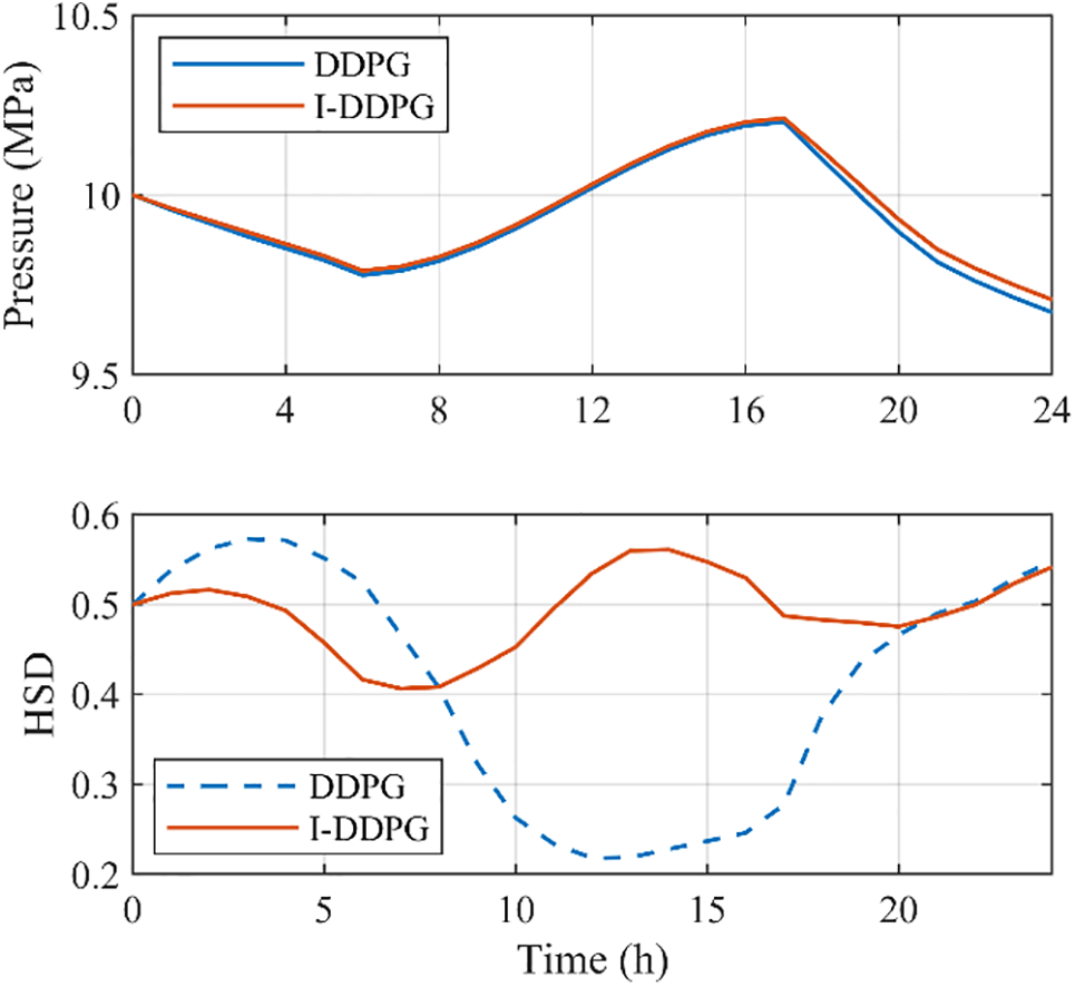
Figure 6: Comparison of state changes of energy storage devices

Fig. 7 demonstrates the power balance characteristics of the I-DDPG algorithm under typical daytime scenarios. It can be observed through the power balance diagram that the algorithm exhibits significant strategy differentiation under different PV conditions: during the nighttime PV-free hours, the system adopts a conservative energy management strategy, through dynamically optimizing the output curve of the fuel cell, to satisfy the demand of the base electric load while controlling the power generation of the fuel cell at a lower level, and actively reducing the power consumption of the heat pump, so as to achieve efficient distribution of electric energy. When the PV output is sufficient, the system switches to PV priority mode: firstly, the PV power is fully consumed, most of which is stored through hydrogen production in the electrolyzer, and the remaining small part of electricity is directly supplied to the electric load and heat pump. This phase avoids frequent start/stop of the fuel cell and significantly extends the equipment life.

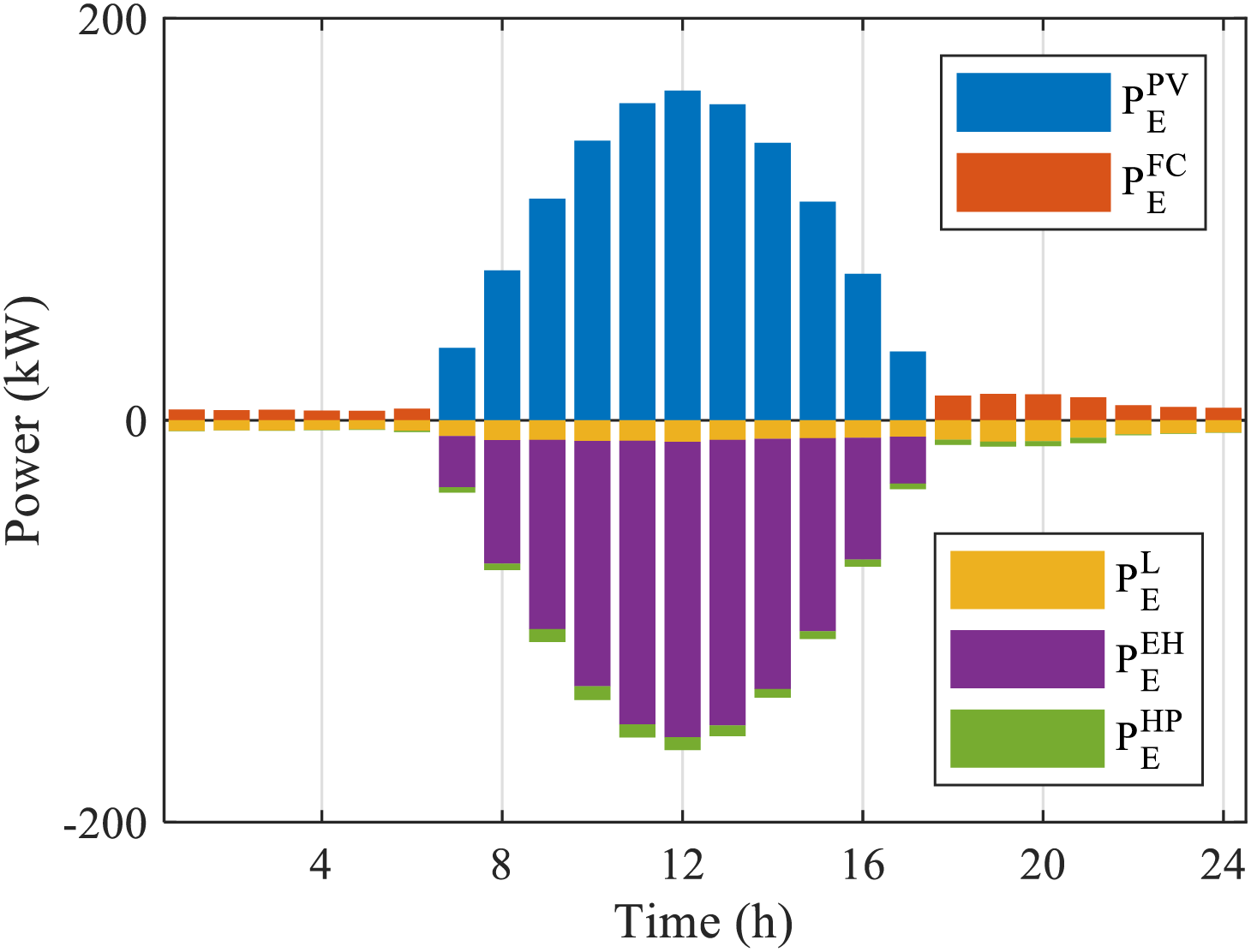
Figure 7: Electrical balance diagram for typical day scenario

The heat balance analysis in Fig. 8 further reveals the multi-energy coupling characteristics. In the case of no PV, the system constructs a double guarantee mechanism of “fuel cell waste heat + heat release from the storage tank”, in which the heat release strategy of the storage tank reduces the heat supply pressure of the fuel cell. When the PV is available, the system utilizes the high COP value of the heat pump in that period to generate a large amount of heat and supplement the heat storage tank. In summary, the I-DDPG has significant energy management optimization capability, which can efficiently achieve reasonable storage and timely distribution of energy, and ensure the continuity and stability of power and heat supply under different lighting conditions.

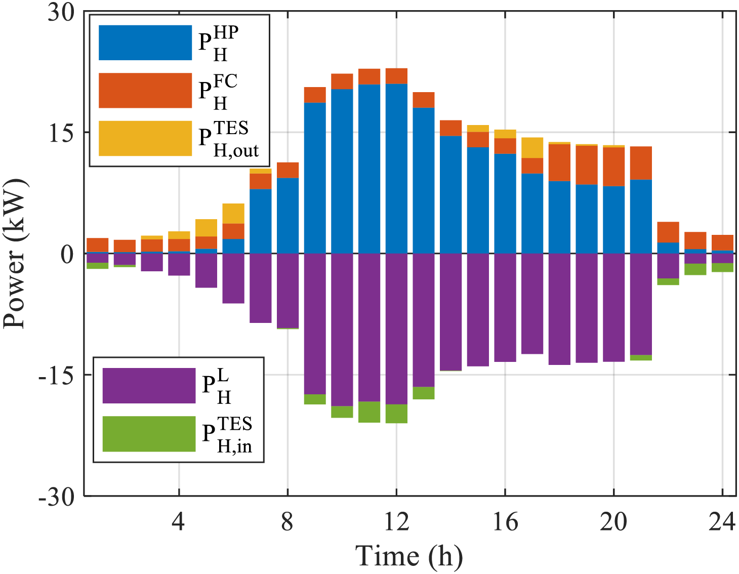
Figure 8: Heat balance diagram for typical day scenario

4.3 Performance Analysis of Multiple Algorithms under Stochastic Conditions

To verify the performance of the proposed I-DDPG in terms of robustness and performance advantages, this study conducts an in-depth performance analysis of the I-DDPG, the original algorithm, and the rule-based algorithm under various uncertainty scenarios. Specifically, different levels of random volatility, i.e., 10% volatility, 20% volatility, and 30% volatility, are introduced on the basis of typical daily scenarios, and thirty sets of test scenarios are randomly generated based on these volatility levels. Subsequently, the performance of the three algorithms is exhaustively analyzed and compared under these thirty sets of test scenarios. The results of the relevant performance analysis and comparison are presented in Table 3.

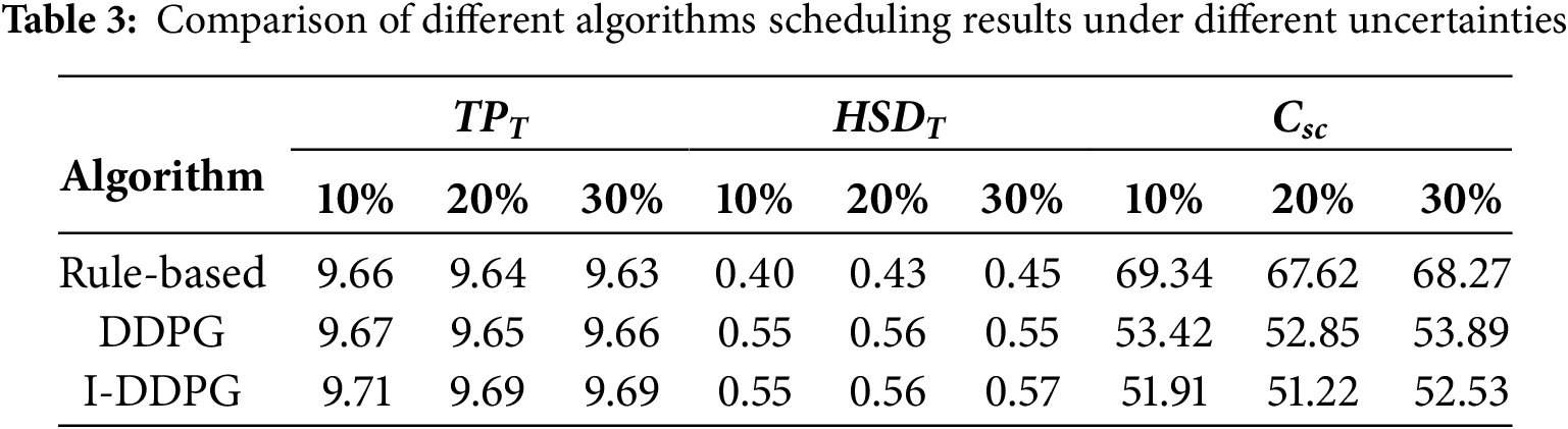
Table 3 demonstrates the average performance metrics of different algorithms under each uncertainty level. The analysis results show that both the DDPG and I-DDPG algorithms exhibit superior control in the hydrogen storage tank pressure regulation task compared to the traditional rule-based approach, and their regulation results are closer to the initial state of scheduling. Further comparing the two reinforcement learning algorithms, the control accuracy of I-DDPG under 10%, 20%, and 30% uncertainty levels is improved by 0.41%, 0.41%, and 0.31%, respectively, compared with that of DDPG, showing stronger robustness. As for the energy storage state of the heat storage tank, the final state of the tank for both algorithms presents similar levels when faced with 10% vs. 20% uncertainty scenarios. However, under the high uncertainty condition of 30%, the I-DDPG algorithm shows a significant advantage in maintaining the energy storage state of the thermal storage tank, and its performance improves by 3.64% compared to the DDPG algorithm, indicating that the I-DDPG has a stronger stability in the extreme uncertainty environment. The indicators in the table combine the system operating cost with the energy storage state of the storage device, which constitutes the integrated cost of dispatch. In terms of the integrated cost of dispatch, I-DDPG achieves cost reductions of 2.82%, 3.08%, and 2.52% for the 10%, 20%, and 30% uncertainty scenarios, respectively, and the average cost reduction over the 30 sets of simulated scenarios is 2.80%.

5  Conclusion

A model for a low-carbon building trigeneration system comprising photovoltaics, electrolytic hydrogen production, hydrogen storage, fuel cells, heat pumps, and thermal storage was created in this study. To optimize the system’s scheduling, an improved I-DDPG algorithm based on the DDPG algorithm was suggested. The primary findings of this study are as follows:

•   Given the numerous uncertainties and intricate multi-energy coupling issues that EHHT faces during actual operation, the MDP model developed in this study can accurately and thoroughly depict the system’s operational characteristics, offer a useful optimization framework for the ensuing reinforcement learning algorithm, and establish a strong theoretical basis for achieving EHHT’s efficient management and optimal scheduling.

•   To optimize the DDPG algorithm, a multiple exploration strategy is presented. The experimental findings show that this improvement measure not only significantly increases the algorithm’s training convergence value by 22.8% and its training convergence speed by 12.5%, but it also confirms the suggested improvement measure’s viability and efficacy.

•   I-DDPG exhibits notable advantages in the final state regulation of energy storage devices and the optimization of integrated dispatch cost when compared and analyzed with the original algorithm and the rule-based algorithm. The suggested algorithm’s robustness in enhancing system economics and managing uncertainty is fully verified by the 2.82%, 3.08%, and 2.52% cost reduction effects it achieves under 10%, 20%, and 30% uncertainty scenarios, respectively, and the 2.80% average cost reduction of the 30 sets of simulated scenarios.

Acknowledgement: We are very grateful for the support of State Grid Jiangsu Electric Power Company.

Funding Statement: The study was supported by the Science and Technology Projects of State Grid Jiangsu Electric Power Company “Design, Regulation and Application of Electric-Hydrogen-Heat Integrated Energy Systems for Low Carbon Buildings, J2024184”.

Author Contributions: Study conception and design: Bin Chen; data collection: Yutong Lei; analysis and interpretation of results: Wei Zhang; draft manuscript preparation: Jiayun Ding. All authors reviewed the results and approved the final version of the manuscript.

Availability of Data and Materials: Due to the nature of this research, participants of this study did not agree for their data to be shared publicly, so supporting data is not available.

Ethics Approval: Not applicable.

Conflicts of Interest: The authors declare no conflicts of interest to report regarding the present study.

References

1. Wang H, Chen W, Shi J. Low carbon transition of global building sector under 2- and 1.5-degree targets. Appl Energy. 2018 Apr;222(2):148–57. doi:10.1016/j.apenergy.2018.03.090. [Google Scholar] [CrossRef]

2. Lu W, Tam VW, Chen H, Du L. A holistic review of research on carbon emissions of green building construction industry. Eng Constr Archit Manag. 2020 Jan;27(5):1065–92. doi:10.1108/ECAM-06-2019-0283. [Google Scholar] [CrossRef]

3. Ochoa-Correa D, Arévalo P, Villa-Ávila E, Espinoza JL, Jurado F. Feasible solutions for low-carbon thermal electricity generation and utilization in oil-rich developing countries: a literature review. Fire. 2024 Sep;7(10):344. doi:10.3390/fire7100344. [Google Scholar] [CrossRef]

4. Shakeri Kebria Z, Fattahi P, Setak M. A stochastic multi-period energy hubs through backup and storage systems: enhancing cost efficiency, and sustainability. Clean Technol Environ Policy. 2023 Dec;26(4):1049–73. doi:10.1007/s10098-023-02660-7. [Google Scholar] [CrossRef]

5. Yao W, Chen X, Luo W, van Tooren M, Guo J. Review of uncertainty-based multidisciplinary design optimization methods for aerospace vehicles. Prog Aerosp Sci. 2011 Jul;47(6):450–79. doi:10.1016/j.paerosci.2011.05.001. [Google Scholar] [CrossRef]

6. Sahinidis NV. Optimization under uncertainty: state-of-the-art and opportunities. Comput Chem Eng. 2003 Nov;28(6–7):971–83. doi:10.1016/j.compchemeng.2003.09.017. [Google Scholar] [CrossRef]

7. Li X, Wen J. Review of building energy modeling for control and operation. Renew Sustain Energy Rev. 2014 Jun;37(9):517–37. doi:10.1016/j.rser.2014.05.056. [Google Scholar] [CrossRef]

8. Sterman JD. All models are wrong: reflections on becoming a systems scientist. Syst Dyn Rev. 2002 Dec;18(4):501–31. doi:10.1002/sdr.261. [Google Scholar] [CrossRef]

9. Nguyen AT, Reiter S, Rigo P. A review on simulation-based optimization methods applied to building performance analysis. Appl Energy. 2013 Sep;113(2):1043–58. doi:10.1016/j.apenergy.2013.08.061. [Google Scholar] [CrossRef]

10. A.Shah MI, Wahid A, Barrett E, Mason K. Multi-agent systems in Peer-to-Peer energy trading: a comprehensive survey. Eng Appl Artif Intell. 2024 Jan;132(8):107847. doi:10.1016/j.engappai.2024.107847. [Google Scholar] [CrossRef]

11. Nguyen TT, Nguyen ND, Nahavandi S. Deep reinforcement learning for multiagent systems: a review of challenges, solutions, and applications. IEEE Trans Cybern. 2020 Mar;50:3826–39. doi:10.1109/tcyb.2020.2977374. [Google Scholar] [PubMed] [CrossRef]

12. Hewing L, Wabersich KP, Menner M, Zeilinger MN. Learning-based model predictive control: toward safe learning in control. Annu Rev Control Robot Auton Syst. 2019 Dec;3(1):269–96. doi:10.1146/annurev-control-090419-075625. [Google Scholar] [CrossRef]

13. Shengren H, Vergara PP, Duque EMS, Palensky P. Optimal energy system scheduling using a constraint-aware reinforcement learning algorithm. J Electr Eng Technol. 2023 May;152(1):109230. doi:10.1016/j.ijepes.2023.109230. [Google Scholar] [CrossRef]

14. Ye J, Wang X, Hua Q, Sun L. Deep reinforcement learning based energy management of a hybrid electricity-heat-hydrogen energy system with demand response. Energy. 2024 May;305(3):131874. doi:10.1016/j.energy.2024.131874. [Google Scholar] [CrossRef]

15. Li Q, Hua Q, Wang C, Khosravi A, Sun L. Thermodynamic and economic analysis of an off-grid photovoltaic hydrogen production system hybrid with organic Rankine cycle. Appl Therm Eng. 2023 Jun;230:120843. doi:10.1016/j.applthermaleng.2023.120843. [Google Scholar] [CrossRef]

16. Bi X, Wang G, Cui D, Qu X, Shi S, Yu D, et al. Simulation study on the effect of temperature on hydrogen production performance of alkaline electrolytic water. Fuel. 2024 Sep;380(3):133209. doi:10.1016/j.fuel.2024.133209. [Google Scholar] [CrossRef]

17. Zheng J, Zhang X, Xu P, Gu C, Wu B, Hou Y. Standardized equation for hydrogen gas compressibility factor for fuel consumption applications. Int J Hydrogen Energy. 2016 Apr;41(15):6610–7. doi:10.1016/j.ijhydene.2016.03.004. [Google Scholar] [CrossRef]

18. Wang C, Li Q, Wang C, Zhang Y, Zhuge W. Thermodynamic analysis of a hydrogen fuel cell waste heat recovery system based on a zeotropic organic Rankine cycle. Energy. 2021 May;232(4):121038. doi:10.1016/j.energy.2021.121038. [Google Scholar] [CrossRef]

19. Li C, Yang J, Xia L, Sun X, Wang L, Chen C, et al. Selection of refrigerant based on multi-objective decision analysis for different waste heat recovery schemes. Chin J Chem Eng. 2024 Dec;77(9):236–47. doi:10.1016/j.cjche.2024.09.013. [Google Scholar] [CrossRef]

20. Pau M, Cunsolo F, Vivian J, Ponci F, Monti A. Optimal scheduling of electric heat pumps combined with thermal storage for power peak shaving. In: 2018 IEEE International Conference on Environment and Electrical Engineering and 2018 IEEE Industrial and Commercial Power Systems Europe (EEEIC/I&CPS Europe); 2018 Oct; Palermo, Italy. p. 1–6. doi:10.1109/EEEIC.2018.8494592. [Google Scholar] [CrossRef]

21. Sun L, Jin Y, Shen J, You F. Sustainable residential micro-cogeneration system based on a fuel cell using dynamic programming-based economic day-ahead scheduling. ACS Sustain Chem Eng. 2021 Feb;9(8):3258–66. doi:10.1021/acssuschemeng.0c08725. [Google Scholar] [CrossRef]

22. Wang X, Dong J, Sun L. Deep reinforcement learning based energy scheduling of a hybrid electricity/heat/hydrogen energy system. In: Applied Energy Symposium 2023: Clean Energy towards Carbon Neutrality (CEN2023); 2023 Apr 23–25; Ningbo, China. doi:10.46855/energy-proceedings-10500. [Google Scholar] [CrossRef]