A Bi-Level Optimization Model and Hybrid Evolutionary Algorithm for Wind Farm Layout with Different Turbine Types

1  Introduction

Wind energy, as one of the most commercially promising renewable energy sources, plays an increasingly important role in global energy systems. According to the Global Wind Energy Council (GWEC), the cumulative global wind power installed capacity exceeded 1021 GW in 2023 and is projected to reach 1021 GW by 2025. However, wind energy production is influenced by multiple factors, including surface roughness, wind shear coefficient, turbulence intensity, and wake effects. The wake effect refers to the phenomenon where the rotating blades of an upstream turbine disturb the airflow, leading to reduced downstream wind speed and increased turbulence intensity. This effect significantly impacts the power generation efficiency of downstream turbines, reducing the total output power of the entire wind farm. The Jensen [1] and Larsen wake models are widely used due to their simplicity and efficiency. Computational fluid dynamics (CFD) models [2] are employed to simulate complex flow dynamics in wind farms, offering higher accuracy but at a greater computational cost, making them suitable for detailed analysis. Additionally, accurately evaluating wind power resources [3] and simulating the effects of complex terrain on wind flow remain challenging problems [4]. Consequently, micro-siting for wind farms is a complex task. The mathematical model for wind farm micro-siting is a constrained nonlinear optimization problem, tailored to the preferences of decision-makers. For example, Grady et al. [5] minimized the cost of energy as the optimization objective, while others established single-objective models to maximize output power [6]. Milyani et al. [7] developed a multi-objective optimization model to minimize the levelized cost of electricity and noise levels, and Ling et al. [8] proposed a bi-objective optimization model to maximize power generation while minimizing streamwise turbulence intensity.

However, the aforementioned studies primarily consider wind farm layouts using the same type of wind turbines and often ignore the influence of complex terrain, which reduces the economic efficiency of wind energy. The output power of wind farms can be significantly diminished when general optimization models are applied. Regions with complex topographic conditions complicate wind flow patterns, prompting researchers to seek more effective solutions [9,10]. In recent years, researchers have explored mixed installations of wind turbines to mitigate wake effects. For instance, Chen et al. [11] demonstrated that varying hub heights can reduce costs more effectively than using turbines of the same height in complex terrains. Biswas et al. [12] incorporated rotor diameters and hub heights as key factors in their optimization model to minimize the impact of wake effects on power generation. Tang et al. [13] designed a single-objective model to improve wind farm efficiency, incorporating hub heights, rotor diameters, and cost models for different turbine types. The mixed installation strategy is now being applied in both onshore and offshore wind farms [14,15].

Wind farm optimization models are characterized by nonlinearity, high dimensionality, and high computational complexity. Traditional optimization algorithms struggle to find optimal layouts, leading to the adoption of swarm intelligence algorithms. For example, Emami et al. [16] used a binary-coded genetic algorithm (GA) to minimize the cost per unit of power output and optimize the number and layout of turbines. The teaching-learning-based optimization method has been applied to turbine positioning [17], while a modified greedy algorithm was used to optimize energy conversion efficiency [18]. Yu et al. [19] enhanced the mutation strategy of differential evolution (DE) using local information, overcoming the tendency of classical DE to become trapped in local optima. Hakli [20] employed an artificial bee colony algorithm to solve turbine placement problems, and a hybrid evolutionary algorithm combining particle swarm optimization and GA was used to maximize output power [21].

Existing research primarily employs evolutionary algorithms for wind farm deployment or adopts multiple turbine heights and hybrid installations to reduce wake effects in complex terrains. However, critical challenges remain in wind farm layout optimization, particularly in balancing the dual objectives of minimizing energy production costs and maximizing economic returns. Specifically, the types of wind turbines and their micro-siting significantly influence the output power of wind farms. The interaction between these factors makes a bi-level constrained optimization model particularly advantageous. Therefore, this paper establishes a novel bi-level constrained optimization model to decouple cost functions and output power. The main innovations are as follows:

(1) First, a novel bi-level constrained optimization model is established that is closer to real-world optimization scenarios. The upper-level optimization focuses on turbine-type selection, with relevant parameters including power generation capacity, hub height variations, and cost characteristics. The lower-level optimization model addresses the micro-siting of wind turbines, constrained by surface roughness variations and inter-turbine wake interactions.

(2) A hybrid evolutionary algorithm is designed to solve the bi-level optimization model proposed in this paper. An improved genetic algorithm (GA) is used for upper-level turbine-type selection, while an enhanced differential evolution (DE) algorithm is employed for lower-level micro-siting. The DE algorithm incorporates a mutation operator based on local optimal design and adaptive parameter values, which enhances its exploration capabilities.

This paper is organized as follows. A bi-level constraint optimization model is introduced in Section 2; Then, a hybrid evolutionary algorithm based on genetic algorithm and differential evolution is proposed in Section 3; Next, Section 5 evaluates the experimental results; Finally, Section 6 is the conclusion.

2  Optimization Model

This section first describes the common problems of wind farm optimization; Then, model assumptions and problem formulation are made for the wind farm deployment problem; Finally, according to the characteristics of the problem, a bi-level constraint optimization model is established.

2.1 Prerequisite Knowledge

2.1.1 Wake Effect

Wind farm wake effect refers to the resistance of upstream wind turbines leading to the reduction of wind speed of downstream wind turbines, which affects the economic benefits of wind farms. The key factors of the wake effect are complex, such as the distance between wind turbines, initial wind speed, upstream and downstream wind speed, and the height of wind turbine, etc., which should be considered for the more accurate evaluation of the total power output. Computational fluid dynamics (CFD) models are high-fidelity models that solve the Navier-Stokes equations to simulate the complex flow dynamics in a wind farm. While highly accurate, it is computationally expensive and typically used for detailed analysis. Therefore, some simplified linear wake models are usually used in wind turbine layout optimization, the Jensen wake model [1] is a widely used analytical model developed by Niels Otto Jensen in the 1980s. It is a simple yet effective model for predicting the velocity deficit in the wake of a wind turbine. Key Assumptions of the Jensen Model include (a): The wake expands linearly downstream of the turbine; (b) The velocity deficit in the wake is uniform across the wake cross-section; (c) The wake is axisymmetric (circular in cross-section); (d) The model assumes a constant turbulence intensity and neutral atmospheric conditions. An improved linear wake model proposed by Chen et al. [11] is adopted in this paper. As shown in Fig. 1, suppose that the location of the i-th wind turbine and the j-th wind turbine are denoted as A and B, respectively, then the velocity deficit of wind turbine i-this calculated by follows:

ρ=0.5(1−1−α),β=0.5ln⁡(H/H0),(1)

VDi,j=2ρ(1+βDi,j/Rj)2,(2)

where α is the axial induction factor, Cr is the thrust coefficient [15], Hj is the tower height of wind turbine j, β is the constant, Vi and Vj are respectively the wind speed of wind turbines i and j. Where the terrain’s surface roughness is modeled to account for the impact of vegetation, buildings, and other obstacles on wind flow. Surface roughness values are assigned to different regions of the terrain based on land use data, which influence the wind speed profile. In this paper, the roughness is set to a fixed value, and noted as H0.

Di,j=|(xi−xj)cos⁡θ+(yi−yj)cos⁡θ|.(3)

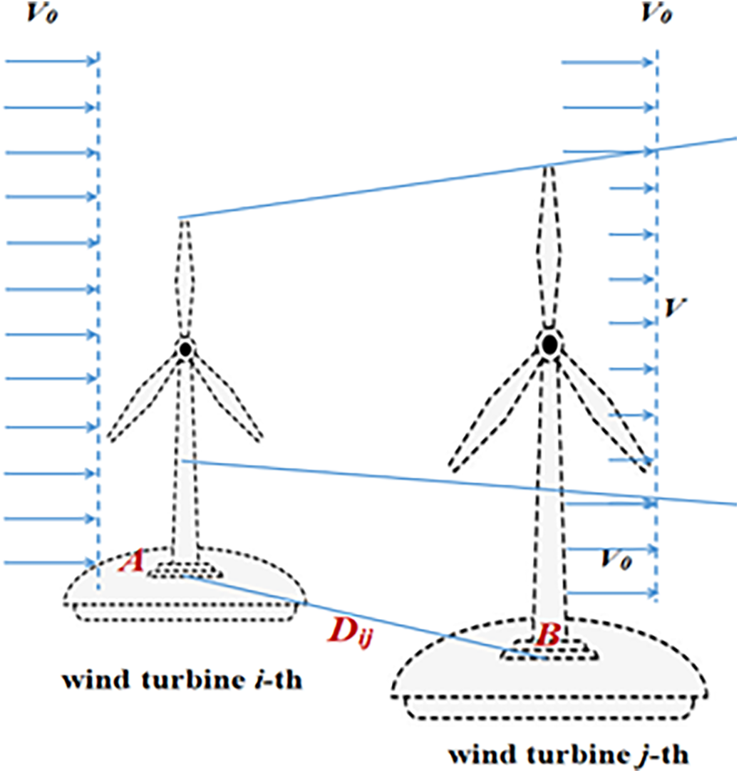
Figure 1: The illustration of the wake effect

The sum of the total velocity deficit wind turbine i is calculated as follows:

VDi=∑j=1,i≠jNVDj,i,j=1,2,⋯,N.(4)

The parameter Ci(θ) of the wind turbine i is updated by the following equation, and noted as Ci′(θ),

Ci′(θ)=Ci(θ)(1−VDi),i=1,2,⋯,N.(5)

2.1.2 Probability Distribution of Wind Speed

Considering the strong randomness of wind speed, the wind speed distribution probability model is generally used to approximately describe its statistical characteristics. It can reflect the probability of each wind speed segment at a certain time of the wind farm. Weibull distribution model is commonly used to fit wind speed distribution, and its probability function is as follows:

F(V)=1−e−VC(θ)K(θ)(6)

The above probability distribution satisfies non-normal distribution, and the corresponding probability density function is:

f(V,C(θ),K(θ))=C(θ)K(θ)(VK(θ))K(θ)−1×e−VC(θ)K(θ),(7)

where V is the wind speed, C(θ) and K(θ) are the scale and shape parameters conditioned on the wind direction θ, respectively, which can be obtained from the empirical values.

2.1.3 The Power Curve

To calculate the output power of the wind farm, a power curve function PV can be used to describe the relationship between the power output P and wind speed V. The nonlinear curvature curve equation proposed by Long et al. [22] is used in this section, and the specific equation is shown as follows:

PV={0,ifV≥Vc0orV<Vci;eVβ+γeV,Vc0≤V<Vci;Pr,otherwise.(8)

The power of the above curve is divided into four cases. The wind speed is too low or too high to cause the wind turbine not to work.

2.2 Expected Output Power

The expected output power of wind turbine i is calculated by the following double integral,

E(Pi)=∫02πf(V,C(θ),K(θ))∫0∞PVC(θ)K(θ)(VK(θ))K(θ)−1×e−VC(θ)K(θ)dvdθ,(9)

where f(θ) is the probability density function of θ. The above integral is simplified by combining the four cases of P(V) and the properties of double integrals. However, when wind speed V satisfies the condition Vc0≤V<Vcr, it is difficult to calculate this integral value. Therefore, the Riemann sum is used for simplification, where both wind speed V and wind direction θ are uniformly divided into several equal intervals. Wind speed V is divided into n equal parts, and wind direction θ is divided into m equal parts. Then, the above result is collated as follows:

E(Pi)=∑t=1mωt{Pr×(e−(Vr/C′i((θt−1+θt)/2))K((θt−1+θt)/2)−e−(Vc0/C′i((θt−1+θt)/2))K((θt−1+θt)/2))+∑j=1n(e−(Vj−1/C′i((θt−1+θt)/2))K((θt−1+θt)/2)−e−(Vj/C′i((θt−1+θt)/2))K((θt−1+θt)/2))×e(Vj−1+Vj)/2α+βe(Vj−1+Vj)/2}(10)

where ωt is the frequency value of wind direction θ falling within the interval [θt−1,θt].

2.3 Problem Analysis and Model Assumptions

To reduce the influence of the wake effect on the wind farm as much as possible, this paper adopts different types of wind turbines for mixed installation to maximize economic benefits. Therefore, assuming that the number of wind turbines is N and the type of wind turbines is M, then it is satisfied ∑k=1MNk=N, where Nk denotes the number of wind turbines of the k-th type. This implies that both the types of wind turbines and their micro-locations need to be optimized. There is a coupling relationship between turbine type and micro-location, as different turbines have varying rotor diameters, hub heights, and power curves, which directly affect wake effects and layout optimization. Therefore, a bi-level optimization model offers significant advantages in addressing the problems of turbine type selection and micro-position optimization in wind farms, primarily for the following reasons:

Upper-Level Problem: Turbine type selection is a global decision problem involving the economic analysis of turbine types, quantities, and combinations. Different turbine types have distinct power characteristics, cost structures, and wake effects, which directly influence the overall economic performance of the wind farm.

Lower-Level Problem: Turbine micro-position optimization is a local decision problem that requires optimizing the specific location of each turbine, given the turbine type and quantity, to minimize wake effects and maximize wind energy capture efficiency.

The bi-level optimization model effectively handles this coupling by separately modeling the upper level (turbine type selection) and the lower level (micro-position optimization). The upper-level decisions provide input to the lower level (turbine type and quantity), while the lower-level decisions feed back optimization results (wake effects and generation efficiency) to guide upper-level adjustments.

2.4 Model Building

In this section, a bi-level constrained optimization model is developed based on the requirements of decision-makers and wind farm optimization objectives. The cost of energy (COE) is taken as the upper-level objective function, which is determined by the cost function and the expected output power E(P), while E(P) is taken as the lower-level objective function. The upper-level constraint is the total number of wind turbines, and the lower-level constraints include the distance between turbines and boundary values. Furthermore, the upper-level decision variable is the turbine type, which is discrete, while the lower-level decision variable is the turbine location within the wind farm, which is continuous.

The factors affecting the cost function of the wind farm are relatively complex, including construction cost, installation cost, maintenance cost, land acquisition cost, etc., which makes it impossible to calculate the cost accurately. Therefore, this paper simplifies the cost function and only includes the base cost Cb established based on [23] and the maintenance cost Cm established based on [24].

Cb=∑k=1MCkNk(1−λk+λke−0.00174Nk),(11)

where λk represent the cost attenuation coefficient of the k-th type, Ck represent the cost of the kth type.

Cb=⌊b1eb2N+(b3−b1eb2N)⌋(1−eb4δ)NPrT,(12)

where Pr is the rated power b1,b2,b3,b4 and δ are experienced parameters, which can be obtained in [24], N represents the number of wind turbines, and T is the service life of the wind turbine.

Based on the above cost functions, a bi-level constrained optimization model is established as follows.

{mins(t) COE=Cb+CmT×W×∑i=1NE(Pi)s.t.  ∑k=1MNk=N;maxN(x,y)∑i=1NE(Pi)s.t.  xmin−R≤xi≤xmin+R;ymin−R≤yi≤ymin+R;(xi−xj)2+(yi−xj)2≥5R;i=1,2,⋯,N,j=1,2,⋯,N,(13)

where S(t)={St1,St2,⋯StN} is an N-dimensional vector, Sti represents the installation type of the i-th wind turbine, and Sti∈{1,2,⋯,K}. N(x,y) is an N-dimensional bi-vector and (xj,yj) represents the position where the j-th wind turbine is located in the wind farm. W is the average running time of the wind turbine per year.

3  Hybrid Evolutionary Algorithm

The evolutionary algorithm is based on a swarm intelligence search mechanism. It begins by generating an initial population, then produces offspring through information exchange between individuals, and selects superior individuals for the next generation based on their fitness values. The optimal solution is obtained through iterative processes until the stopping criterion is satisfied. Typical evolutionary algorithms include the genetic algorithm (GA) [25] and differential evolution (DE) [26], among others. GA simulates the crossover and mutation of biological chromosomes to generate offspring. Its simple crossover operation is well-suited for discrete random variables, making it ideal for the upper-level optimization process in the proposed bi-level optimization model. DE, unlike other evolutionary algorithms, treats individuals as vectors and generates new individuals through vector operations, enabling fast convergence and making it suitable for lower-level optimization. Based on this analysis, a hybrid optimization algorithm combining GA and DE is established in this section.

3.1 Improved Genetic Algorithm

This section first introduces the process of the classical GA, analyzes its limitations, and then presents the improved strategy and detailed steps.

3.1.1 Classic Genetic Algorithm

GA is a class of search techniques inspired by simplified biological processes. Its evolution process consists of four stages:

Initialization: An initial population is randomly generated, where each individual is referred to as a chromosome.

Fitness Evaluation: In each generation, individuals are evaluated based on their fitness values, and high-quality individuals are selected using roulette wheel selection.

Crossover: Parent individuals are selected from the pool for reproduction. One or more points are randomly chosen to exchange genetic material, recombining the genes of the parents to form high-quality offspring.

Mutation: One or more gene loci of the crossover individuals are mutated, simulating biological population variation to create mutated individuals.

Selection: The next generation is selected from the parent and offspring individuals using greedy selection.

Classical genetic algorithms (GA) often use fixed crossover and variation rates, which makes it difficult to balance Exploration and Exploitation at the end of the iteration. When the population tends to converge, the higher crossover rate may destroy the high-quality gene combination, while the lower crossover rate is difficult to escape the local optimal solution. Therefore, the crossover rate and mutation rate are adjusted self-adaptively according to the population state to improve the adaptive ability of the algorithm. When the population diversity is high, the higher mutation rate is used to enhance the exploration ability, and when the population tends to converge, the lower mutation rate is used to enhance the development ability. Such as Zhang et al. proposed an adaptive genetic algorithm [27] based on reinforcement learning that dynamically adjusts parameters through reinforcement learning. An adaptive genetic algorithm is designed for UAV path planning in [28], and the path planning efficiency is improved by dynamically adjusting parameters. Zheng et al. proposed an adaptive genetic algorithm [29] for wind farm layout optimization to reduce the influence of wake effect by dynamically adjusting parameters.

3.1.2 Improved Strategy

The classical GA uses a fixed crossover rate for mutation operations. However, a fixed crossover rate makes it difficult to balance exploration and exploitation in later iterations. This section uses individual information to design an self-adaptive adjustment strategy to solve the above problem. The specific process is as follows.

Self-adaptive parameters setting: The crossover factor Pc and mutation factor Pm should be related to the quality of the parent individual in GA. If the individual is relatively excellent, the probability of crossover and mutation factors is smaller. Conversely, the values of both should be larger. Therefore, the sample diversity of the population can be defined as

Sd=fmax−favgfmax.(14)

Individual differences can be defined as

Id=f−favgfmax,(15)

where fmax and favg are respectively the maximum and the average fitness value; f is the fitness value of the current individual.

The above results are used to self-adjust the relevant parameters as follows

Pc=0.5+ε,(16)

Pm=0.001+0.002ε,(17)

where ε∼N(μ,δ2), and μ satisfied with

μ=Smax−SdSmax+Imax−IdImax−Imin(18)

where Smax is the maximum value of history Sd. The Imax and Imin are respectively the maximum and minimum of Id in the current population.

3.2 Improved Differential Evolution

This section first introduces the algorithm process of classical DE and then introduces the improved strategy and detailed steps.

3.2.1 Classic Differential Evolution

The iterative process of DE mainly includes four steps: initialization, crossover, mutation, and selection, the detailed process is described as follows.

Initialization: An initialized population of size NP is randomly generated in the decision space, and denoted as X={x1,x2,⋯,xNP}.

Mutation: The best individual or a randomly selected individual is used as the basis vector, the difference between the two individuals is used as the direction vector, and F is used as the scaling factor. The mutation individual is generated by the composite operation between the vectors, i.e.,

•DE/rand/1

vi=xr1+F∗(xr2−xr3),(19)

•DE/best/1

vi=xbest+F∗(xr1−xr2),(20)

where the indices r1,r2,r3 are randomly selected from the set of {1, 2, ..., NP}, Xbest denotes the best individual in the current population.

Crossover: The components of the parent individual and the mutation individual are recombined using the given crossover probability,

uij={vij,ifrand(0,1)<CR orj=jrand;xij,otherwise,(21)

where j = 1, 2, . . . , D. jrand is an integer randomly chosen in [1, D], and (0, 1) is a random number in [0, 1], and CR is called the crossover probability.

Selection: The fitness value is used to select the offspring individual from the parent individual and the corresponding crossover individual.

The classic DE has some shortcomings in parameter sensitivity, local search ability and diversity preservation. The performance and applicability of DE are improved by means of adaptive parameter adjustment, multi-strategy fusion and local search enhancement. Such as Duan et al. proposes a superior-inferior mutation strategy [30] based on the superior individual and inferior individual, this process leads to the discovery of high-quality offspring. Sheng et al. proposed differential evolution algorithm [31] integrates four strategies to solve the multiple roots of nonlinear equation systems. Luo et al. introduce a new hierarchical selection mutation strategy and applies different mutation strategies at different stages of evolution to enhance the DE’s performance [32].

3.2.2 Improved Strategy

The performance of DE is primarily influenced by the mutation operation and the value of the mutation factor F. An effective mutation operation can maintain population diversity and ensure the algorithm’s robustness. Therefore, this section improves the mutation operator and adopts an self-adaptive adjustment strategy to set the mutation factor F.

Self-Adaptive Adjustment: Since the mutation factor F in DE is closely related to the population’s performance, leveraging historical population information to self-adaptively set F can enhance the algorithm’s exploration and exploitation capabilities. The specific steps are described as follows:

Step 1: An external archive set X~ of size s was established to store the historical excellent individuals and the corresponding fitness values.

Step 2: Sort the fitness values stored in X, denoted as R;

Step 3: Compare the values between DG−1 and DG one by one, if the value of DG−1 is greater than the value of DG, it is denoted as 0, otherwise it is denoted as 0. Then the above result forms a vector α→ of length NP;

Step 4: Calculate the proportion of 1’s in this vector, denoted as r, and use r to adjust the variation factor FG+1, i.e.,

FG+1={FG−0.1,ifr≤0.5;FG+0.1,otherwise,(22)

where the mutation factor of the first generation, i.e., the initial value is denoted as F0, and the boundary repair is performed on the above value according to the empirical value,

FG+1={0.2,ifFG+1≤0.2;1.2,ifFG+1≥1.2.(23)

Mutation operator: This section uses the information of the historical population to construct the mutation operator to avoid the algorithm falling into the local optimum. The specific process is divided into the following four steps.

Step 1: An external archive set X~ of size s was established to store the historical excellent;

Step 2: The fitness values stored in X~ are sorted and denoted as R = {R1, R2, ..., Rs};

Step 3: The probability values are set according to the sorting results,

qi=1−Ri∑t=1sRt,i=1,2,⋯,s,(24)

p=qi∑t=1sqt,i=1,2,⋯,s.(25)

Step 4: The historical best individual xpbest is selected by the wheel section to perform the following mutation operation.

vi=xi+F∗(xpbest−xi)+rand∗(xr1−xr2).(26)

In the above equation, and represents a random number in the interval (0, 1).

4  Algorithmic Framework

This section mainly introduces the framework of the hybrid evolutionary algorithm (HEA/GA-DE) proposed in this paper, which is based on improved GA and DE. The framework of the algorithm is shown in Fig. 2.

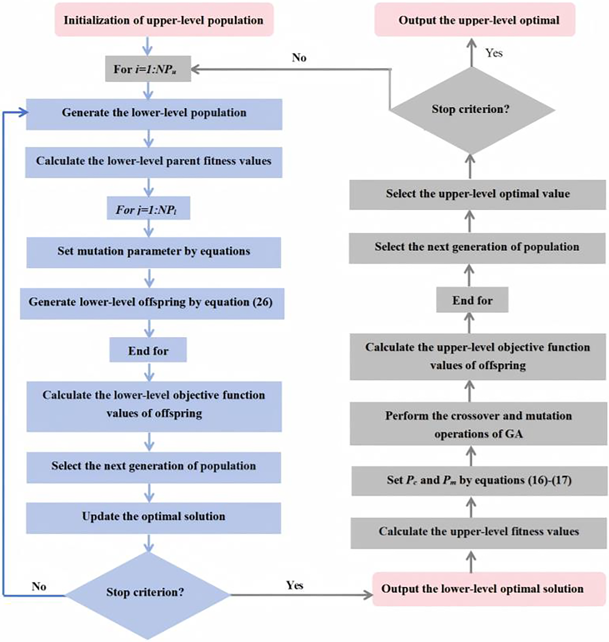
Figure 2: The framework of HEA/GA-DE

The proposed optimization framework operates under a fixed wind farm size and consists of two interdependent levels, where the scale of the number of wind farms is denoted as N. Firstly, The initialization population of the upper-level is generated in a random manner, where each individual encodes wind turbine type configurations; Then, the lower-level initial population is generated according to the upper decision variables and the lower-level constraints; Next, the proposed DE is used to optimize the lower-level objective function. The specific process is described as follows. (i) The objective fitness values of the lower-level are calculated; (ii) Mutation factor is carried out using Eqs. (22) and (23); (iii) Mutation and crossover operations are carried out for the lower-level using Eq. (26) to generate offspring individuals; (iv) The fitness values of offspring individuals are calculated; (v) The selection strategy of DE is used to select the offspring individuals and output the optimal value of the lower-level; (vi) The optimal solution of the lower-level was fed back to the upper-level. Moreover, Genetic algorithm is used to optimize the upper-level objective function. The specific process is described as follows. (I) Calculate the fitness values of the upper parent population; (II) Crossover and mutation operations are carried out for the upper-level using GA; (III) The fitness values of offspring individuals are calculated, and select the offspring individuals; (IV) The upper-level optimal value is selected and stored. Finally, the above process is repeated until the stopping criterion is satisfied, and the optimal solution of the upper-level and lower-level are output.

5  Experimental Analysis

To verify the performance of the hybrid algorithm proposed in this paper, classical GA, a discrete hybrid PSO and GA algorithm [33], DE/rand/1, and improved differential evolution (JADE) [34], are used as comparison algorithms. Where the stopping criterion is the number of evaluations of the maximum fitness, and set as 20,000, the size of the population is set as 100, and the specific parameters are shown in Table 1.

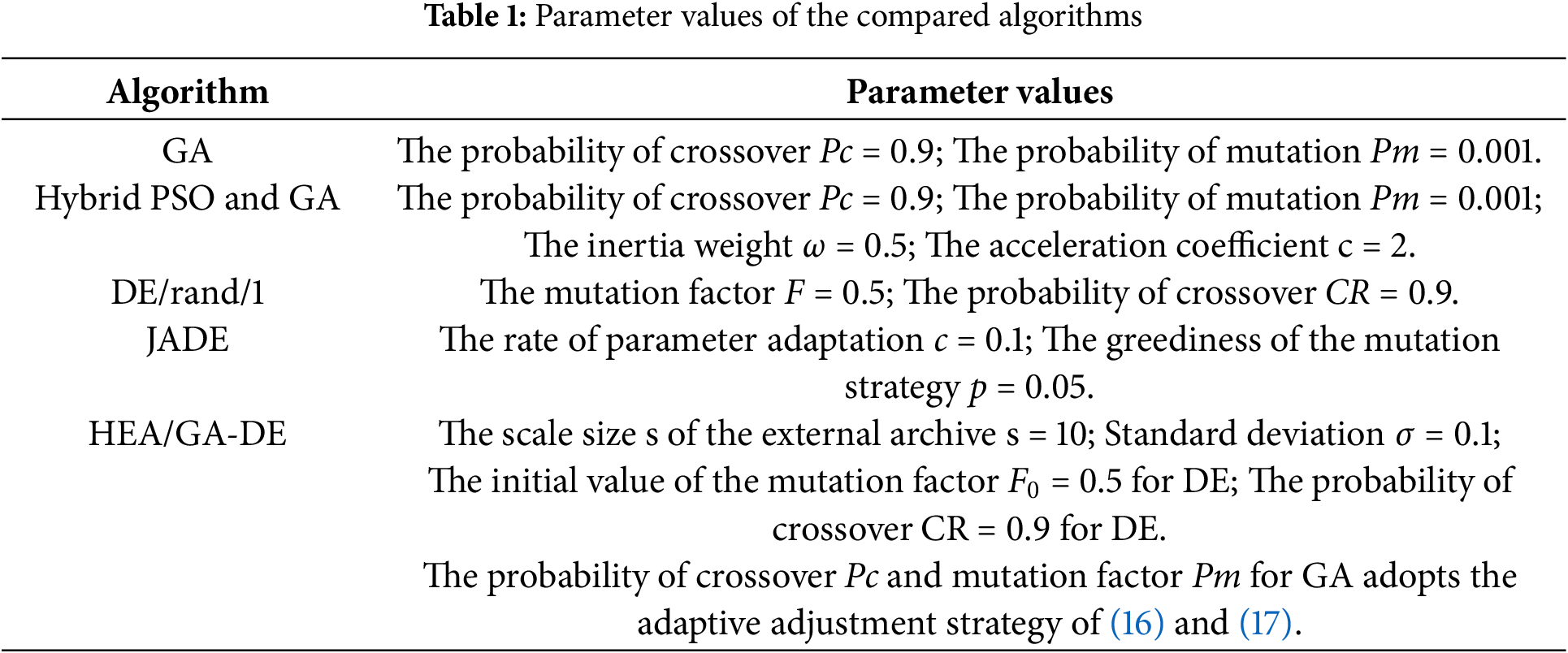
Each algorithm was run 20 times during the simulation experiment, and the mean and standard deviation of the experimental results were recorded.

5.1 Related Parameters

In this paper, the number of wind turbines is generated by the enumeration method when the size of the wind farm is determined, so the size of the wind farm is set as [2000, 2000], [3000, 3000], and [5000, 5000], respectively. Moreover, wind conditions recorded based on historical data are used as the available information to detect the output power of the wind farm. The interval division and corresponding values of wind conditions are shown in Table 2 for the i-th wind turbine, where the value of Ki(θ) set as 2.

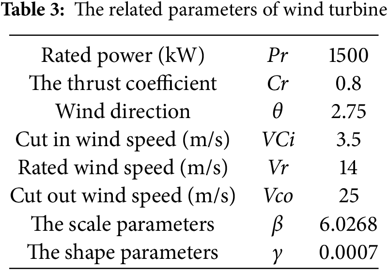
The specifications of the GE1.5-77 wind turbine are shown in Table 3, and the surface roughness H0 are respectively set as 0.003 and 0.01.

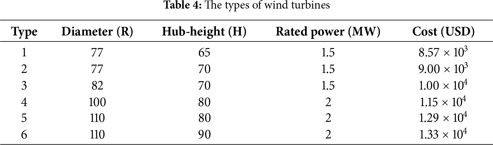
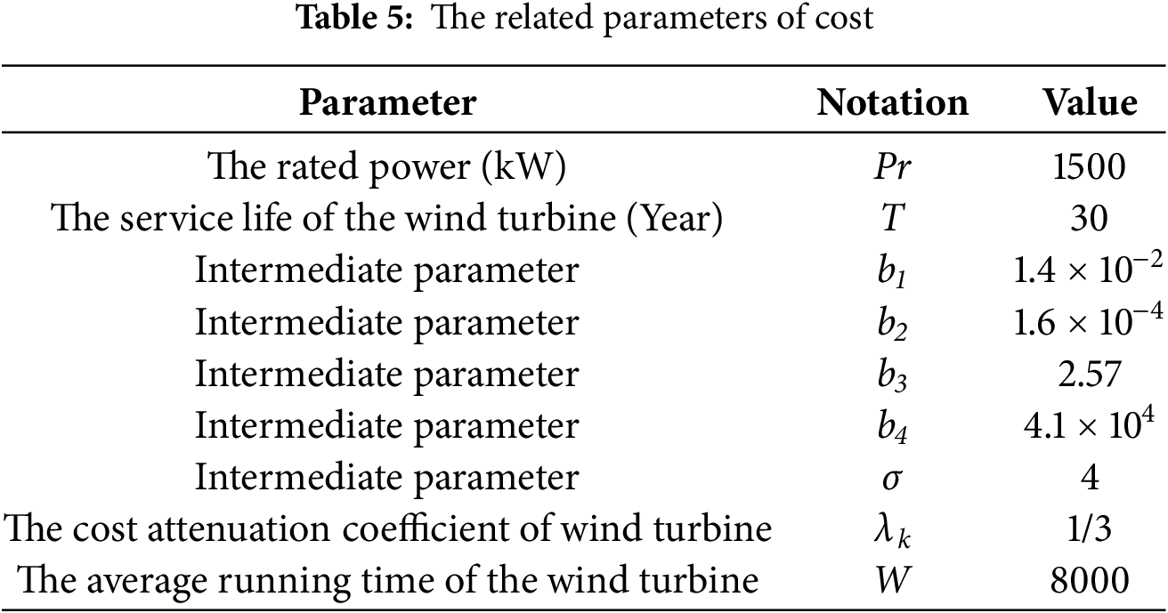
Six different fan types are used in this paper according to the specifications of wind turbines that are installed. The types of wind turbines and related parameters that can be installed in the wind farm are shown in Table 4, and Table 5 lists the relevant parameters of cost.

5.2 Experimental Results and Analysis

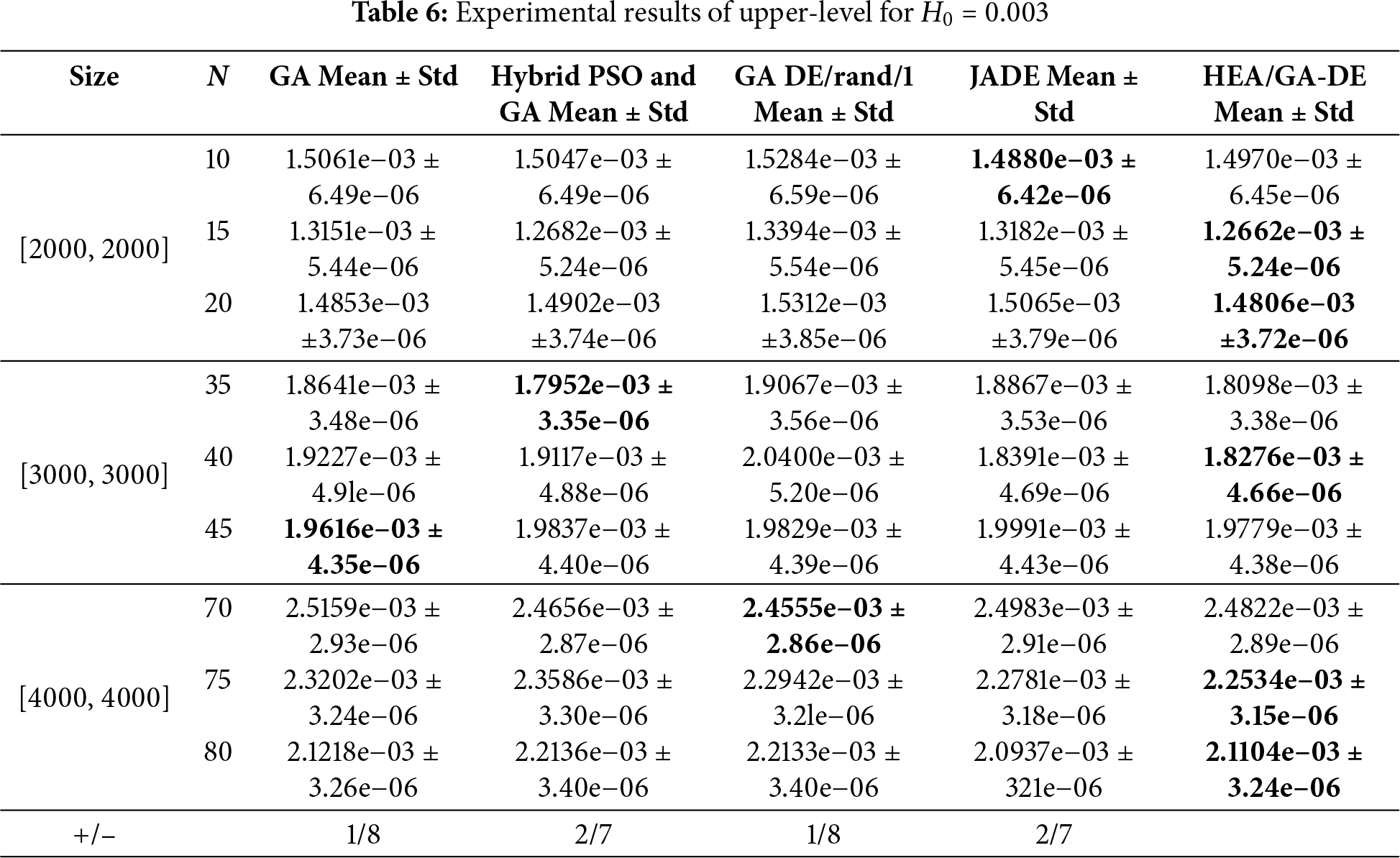
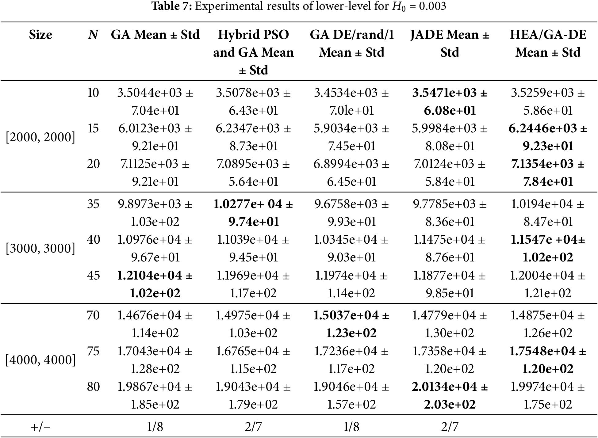
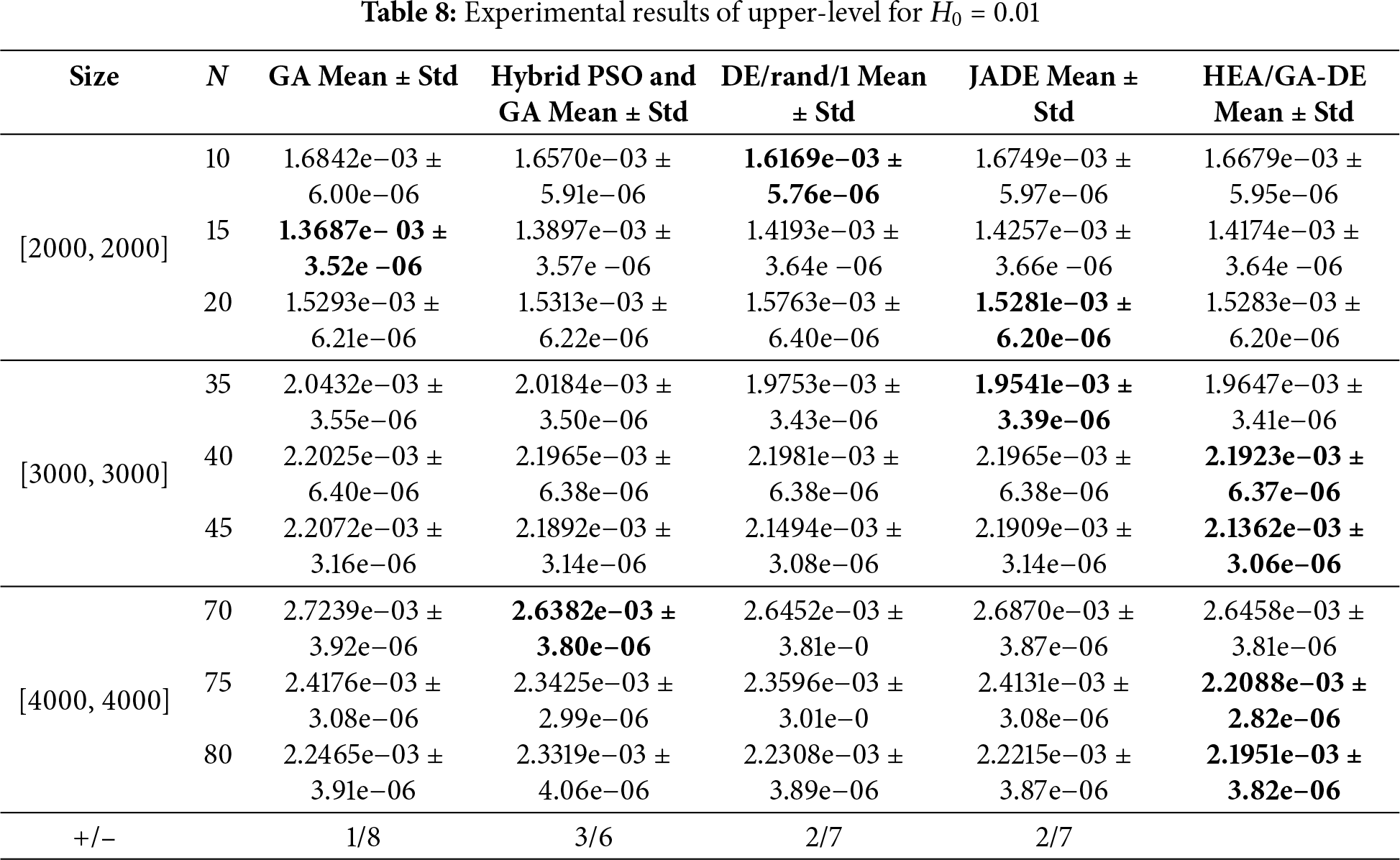
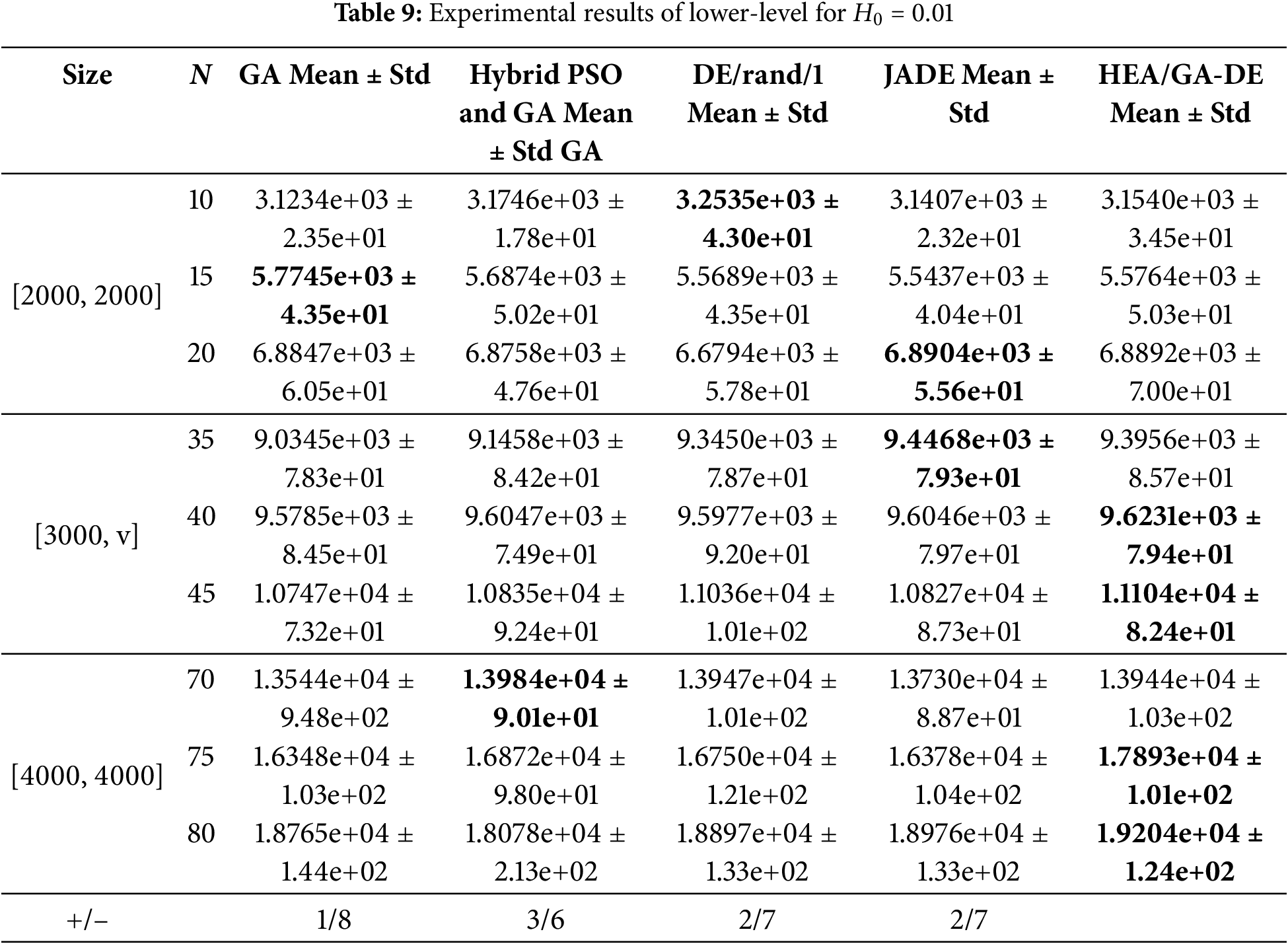
The mean values and standard deviations of upper-level objective and lower-level are shown in Tables 6–9, where “+” and “−” mean that the competition algorithm is better or worse than HEA/GA-DE, respectively. Bold indicates the best results of all compared algorithms. It is worth noting that to verify the performance of the proposed algorithm in solving the bi-level objective function, GA, Hybrid PSO, and GA are only used to optimize the objective function of the upper-level, and the improved DE proposed in this paper is used to optimize the Objective function lower-level. In the same way, DE/rand/1 and JADE are only used to optimize the objective function of lower-level, and the improved GA proposed in this paper is used to optimize the objective function of upper-level.

5.2.1 The Experimental Result of Surface Roughness Is 0.003

Tables 6–7 show the results of the simulation experiments of the compared algorithms when the value of surface roughness is 0.003, where the size of wind turbines are respectively set as 10, 15, 20, 35, 40, 45, 70, 75, and 80. Table 6 counts the mean and standard deviation of the objective function at the upper-level, and Table 7 counts the mean and standard deviation of the objective function at the lower-level.

As shown in the last row of Table 6, the proposed HEA/GA-DE algorithm demonstrates a performance advantage of over 70% compared to other algorithms. Furthermore, for wind farm sizes of [2000, 2000], [3000, 3000], and [4000, 4000], the upper-level objective function values are optimal when the number of installed wind turbines is 15, 20, 40, 75, and 80. Compared to the average values of the competing algorithms, the upper-level objective function values of HEA/GA-DE are reduced by 2.71%, 1.21%, 4.28%, 2.06%, and 1.87%, respectively. This improvement is primarily attributed to the hybrid evolutionary strategies proposed in this paper. Specifically, the upper-level optimization model involves discrete decision variables (wind turbine types), making the discrete GA operator more suitable for optimization. Meanwhile, the lower-level optimization model, which deals with continuous decision variables (wind turbine locations), benefits from the improved DE algorithm due to its powerful global search capability, simple parameter settings, and efficient convergence.

However, for cases with 10, 35, 45, and 70 installed wind turbines, the HEA/GA-DE algorithm does not achieve the best performance. This is mainly due to the uncertainty in wind turbine types, which increases wake effects between turbines. Additionally, the upper-level objective function values tend to increase with larger wind farm scales, primarily because the number of wind turbines is proportional to the overall cost.

The last column of Table 7 indicates that the optimal ratio of the proposed algorithm exceeds 30%. However, some limitations remain. For instance, the improved DE strategy incurs additional computational overhead due to the selection of local optimal solutions. Moreover, the self-adaptive mutation parameter strategy may limit the exploration ability of DE.

5.2.2 The Experimental Result of Surface Roughness Is 0.01

To evaluate the performance of the comparison algorithms in solving the wind farm layout optimization problem under complex terrain conditions, the surface roughness value is adjusted to 0.01 while keeping all other conditions unchanged. The simulation results are presented in Tables 8 and 9.

The last row of Table 9 shows that the dominant proportion of algorithm HEA/GA-DE is substantial. Moreover, as the number of wind turbines increases, the output power also increases. In addition, from the results of the standard deviation, it can be seen that the convergence of these five comparison algorithms is almost no different.

The complexity of the wind farm layout is expensive when the terrain is complex, and the wake effect will be more obvious, therefore, the output power of the wind farm is decreased. This means that the denominator of the upper-level objective function becomes smaller, and this process causes the upper level objective function to become larger.

Although overall, the optimization process of wind farms is full of challenges due to the increasing scale and complex terrain of wind farms, the results in the last row of Tables 8 and 9 show that the performance of HEA/GA-DE is better compared with the compared algorithms.

6  Conclusion

Considering that hybrid installation of different types is beneficial to maximize the benefits of wind farms in complex terrain, a bi-level constrained optimization model is proposed to solve the deployment problem of wind farms in this paper, where the objective functions consider the cost function, wake effect, and output power. Moreover, a hybrid evolutionary algorithm is designed to realize the type and micro-location problem of wind turbines. Finally, four algorithms are used as comparison algorithms, and the effectiveness of the proposed algorithm is verified by some simulation experiments. Experimental results show that the cost per unit of energy (COE) maximum decreased by 5.9%, and the output power maximum increased by 4%. However, the computational complexity of the bi-level optimization model is higher, especially the lower-level optimization part. Future research will focus on exploring the following directions to reduce the computation, and agent model is used to replace part of the high-precision calculation and reduce the optimization time of the lower-level.

Acknowledgement: Not applicable.

Funding Statement: The research work was supported by the National Natural Science Foundation of China [Grant No. 12461035] and Qinghai University Students Innovative Training Program Project [2024-QX-57].

Author Contributions: All authors contributed to the study’s conception and design. The first draft of the manuscript was written by Erping Song. The polishing of the language and the analysis of the data were done by Zipin Yao. All authors reviewed the results and approved the final version of the manuscript.

Availability of Data and Materials: Some or all data and models are available from the corresponding author by request.

Ethics Approval: There are no studies involving human participants or animals in this manuscript.

Conflicts of Interest: The authors declare no conflicts of interest to report regarding the present study.

References

1. Jensen N. A note on wind generator interaction. Roskilde, Denmark: Riso National Laboratory; 1983. [Google Scholar]

2. Makridis A, Chick J. Validation of a CFD model of wind turbine wakes with terrain effects. J Wind Eng Ind Aerodyn. 2013;123(1):12–29. doi:10.1016/j.jweia.2013.08.009. [Google Scholar] [CrossRef]

3. Schmidt J, Stoevesandt B. The impact of wake models on wind farm layout optimization. J Phys Conf Ser. 2015;625:012040. doi:10.1088/1742-6596/625/1/012040. [Google Scholar] [CrossRef]

4. Wang L, Tan ACC, Cholette ME, Gu Y. Optimization of wind farm layout with complex land divisions. Renew Energy. 2017;105(1):30–40. doi:10.1016/j.renene.2016.12.025. [Google Scholar] [CrossRef]

5. Grady SA, Hussaini MY, Abdullah MM. Placement of wind turbines using genetic algorithms. Renew Energy. 2005;30(2):259–70. doi:10.1016/j.renene.2004.05.007. [Google Scholar] [CrossRef]

6. Qureshi TA, Warudkar V. Wind farm layout optimization through optimal wind turbine placement using a hybrid particle swarm optimization and genetic algorithm. Environ Sci Pollut Res Int. 2023;30(31):77436–52. doi:10.1007/s11356-023-27849-7. [Google Scholar] [PubMed] [CrossRef]

7. Hidayat T, Ramli MAM, Hardi AZ, Bouchekara HREH, Milyani AH. Wind farm layout optimization using multiobjective modified electric charged particles optimization algorithm based on game theory indexing in real onshore area. Sustainability. 2024;16(23):10222. doi:10.3390/su162310222. [Google Scholar] [CrossRef]

8. Ling Z, Zhao Z, Liu Y, Liu H, Ali K, Liu Y, et al. Multi-objective layout optimization for wind farms based on non-uniformly distributed turbulence and a new three-dimensional multiple wake model. Renew Energy. 2024;227(6–1):120558. doi:10.1016/j.renene.2024.120558. [Google Scholar] [CrossRef]

9. Azlan F, Kurnia JC, Tan BT, Ismadi MZ. Review on optimisation methods of wind farm array under three classical wind condition problems. Renew Sustain Energy Rev. 2021;135:110047. doi:10.1016/j.rser.2020.110047. [Google Scholar] [CrossRef]

10. Croonenbroeck C, Hennecke D. A comparison of optimizers in a unified standard for optimization on wind farm layout optimization. Energy. 2021;216:119244. doi:10.1016/j.energy.2020.119244. [Google Scholar] [CrossRef]

11. Chen K, Song MX, Zhang X, Wang SF. Wind turbine layout optimization with multiple hub height wind turbines using greedy algorithm. Renew Energy. 2016;96(1):676–86. doi:10.1016/j.renene.2016.05.018. [Google Scholar] [CrossRef]

12. Biswas PP, Suganthan PN, Amaratunga GAJ. Optimization of wind turbine rotor diameters and hub heights in a windfarm using differential evolution algorithm. In: Proceedings of Sixth International Conference on Soft Computing for Problem Solving; 2017; Singapore. p. 131–41. doi:10.1007/978-981-10-3325-4_13. [Google Scholar] [CrossRef]

13. Tang X, Yang Q, Wang K, Stoevesandt B, Sun Y. Optimisation of wind farm layout in complex terrain via mixed-installation of different types of turbines. IET Renew Power Gener. 2018;12(9):1065–73. doi:10.1049/iet-rpg.2017.0787. [Google Scholar] [CrossRef]

14. Zhu J, Lin S, Wen J, Qin J, Yan W, Xu B. Discrete multi-height wind farm layout optimization for optimal energy output. In: Advances in artificial intelligence and security. Cham, Switzerland: Springer International Publishing; 2021. p. 245–56. doi:10.1007/978-3-030-78615-1_21. [Google Scholar] [CrossRef]

15. Ziyaei P, Khorasanchi M, Sayyaadi H, Sadollah A. Minimizing the levelized cost of energy in an offshore wind farm with non-homogeneous turbines through layout optimization. Ocean Eng. 2022;249(3):110859. doi:10.1016/j.oceaneng.2022.110859. [Google Scholar] [CrossRef]

16. Emami A, Noghreh P. New approach on optimization in placement of wind turbines within wind farm by genetic algorithms. Renew Energy. 2010;35(7):1559–64. doi:10.1016/j.renene.2009.11.026. [Google Scholar] [CrossRef]

17. Modi YD, Patel J, Nagababu G, Jani HK. Wind farm layout optimization using teaching learning based optimization technique considering power and cost. In: Renewable energy and climate change. Singapore: Springer; 2019. p. 11–22. doi:10.1007/978-981-32-9578-0_2. [Google Scholar] [CrossRef]

18. Quan N, Kim HM. Greedy robust wind farm layout optimization with feasibility guarantee. Eng Optim. 2019;51(7):1152–67. doi:10.1080/0305215x.2018.1509962. [Google Scholar] [CrossRef]

19. Yu Y, Zhang T, Lei Z, Wang Y, Yang H, Gao S. A chaotic local search-based LSHADE with enhanced memory storage mechanism for wind farm layout optimization. Appl Soft Comput. 2023;141(1):110306. doi:10.1016/j.asoc.2023.110306. [Google Scholar] [CrossRef]

20. Hakli H. The optimization of wind turbine placement using a binary artificial bee colony algorithm with multi-dimensional updates. Electr Power Syst Res. 2023;216:109094. doi:10.1016/j.epsr.2022.109094. [Google Scholar] [CrossRef]

21. Lackner MA, Elkinton CN. An analytical framework for offshore wind farm layout optimization. Wind Eng. 2007;31(1):17–31. doi:10.1260/030952407780811401. [Google Scholar] [CrossRef]

22. Long H, Zhang Z. A two-echelon wind farm layout planning model. IEEE Trans Sustain Energy. 2015;6(3):863–71. doi:10.1109/TSTE.2015.2415037. [Google Scholar] [CrossRef]

23. Mosetti G, Poloni C, Diviacco B. Optimization of wind turbine positioning in large windfarms by means of a genetic algorithm. J Wind Eng Ind Aerodyn. 1994;51(1):105–16. doi:10.1016/0167-6105(94)90080-9. [Google Scholar] [CrossRef]

24. Kiranoudis CT, Voros NG, Maroulis ZB. Short-cut design of wind farms. Energy Policy. 2001;29(7):567–78. doi:10.1016/S0301-4215(00)00150-6. [Google Scholar] [CrossRef]

25. Ribeiro Filho JL, Treleaven PC, Alippi C. Genetic-algorithm programming environments. Computer. 1994;27(6):28–43. doi:10.1109/2.294850. [Google Scholar] [CrossRef]

26. Storn R, Price K. Differential evolution a simple and efficient heuristic for global optimization over continuous spaces. J Global Optim. 1997;11(4):341–59. doi:10.1023/A:1008202821328. [Google Scholar] [CrossRef]

27. Zhang X, Chen Y. Reinforcement learning-driven adaptive genetic algorithm for real-time optimization. Neural Comput Appl. 2023;35(4):3215–30. [Google Scholar]

28. Xue Y, Chang Y, Zhang Y, Sun J, Ji Z, Li H, et al. UAV signal recognition of heterogeneous integrated KNN based on genetic algorithm. Telecommun Syst. 2024;85(4):591–9. doi:10.1007/s11235-023-01099-x. [Google Scholar] [CrossRef]

29. Zheng T, Li H, He H, Lei Z, Gao S. An adaptive strategy-incorporated integer genetic algorithm for wind farm layout optimization. J Bionic Eng. 2024;21(3):1522–40. doi:10.1007/s42235-024-00498-3. [Google Scholar] [CrossRef]

30. Duan M, Yu C, Wang S, Li B. A differential evolution algorithm with a superior-inferior mutation scheme. Soft Comput. 2023;27(23):17657–86. doi:10.1007/s00500-023-09038-3. [Google Scholar] [CrossRef]

31. Sheng M, Ding W, Sheng W. Differential evolution with adaptive niching and reinitialisation for nonlinear equation systems. Int J Syst Sci. 2024;55(10):2172–86. doi:10.1080/00207721.2024.2337039. [Google Scholar] [CrossRef]

32. Luo Z, Qian X, Song W. Enhanced differential evolution with hierarchical selection mutation and distance-based selection strategy. Eng Appl Artif Intell. 2025;144(1):110124. doi:10.1016/j.engappai.2025.110124. [Google Scholar] [CrossRef]

33. Omidinasab F, Goodarzimehr V. A hybrid particle swarm optimization and genetic algorithm for truss structures with discrete variables. J Appl Comput Mech. 2020;6(3):593–604. doi:10.22055/jacm.2019.28992.1531. [Google Scholar] [CrossRef]

34. Zhang J, Sanderson AC. JADE: adaptive differential evolution with optional external archive. IEEE Trans Evol Comput. 2009;13(5):945–58. doi:10.1109/TEVC.2009.2014613. [Google Scholar] [CrossRef]