Short-Term Wind Power Forecast Based on STL-IAOA-iTransformer Algorithm: A Case Study in Northwest China

1  Introduction

In recent years, there has been a significant advancement in the development of renewable energy sources [1]. Wind energy, in particular, has gained prominent attention due to its accessibility and efficient energy output [2,3]. As a result, wind power generation has become a key role in the new energy landscape in many countries [4]. However, due to the inherent variability and intermittency of wind power generation [5–7], developing an accurate prediction of wind power generation is essential to ensure the safe and stable operation of power systems [8]. According to the prediction time, the short-term wind power forecast (WPF) involves forecasting active power from 00:00 the next day to 72 h in advance [9]. These predictions can help power companies enhance generation plans, and ensure the safe and stable operation of the power system while reducing spare capacity and operating costs.

Classified by the prediction method, WPF techniques can be typically categorized into the following three aspects: physical, statistical, and hybrid methods [10,11]. Specifically, physical methods utilize local wind data including wind speed, wind direction, and other meteorological data from numerical weather prediction to predict wind power [12,13]. Physical methods in the field of wind power prediction have become relatively mature. For example, reference [14] and reference [15] both used numerical weather forecasts as input data and predicted the short-term wind power generation by Kalman filtering and machine learning (ML) method, respectively. However, creating numerical weather forecast models is usually a complex, costly, and time-consuming process, which makes them impractical for predicting short-term wind speeds [16]. On the other hand, statistical methods extract the relationship between historical wind and generation data for short-term WPFs [17]. ML methods in statistic methods, such as artificial neural networks (ANN) [18], support vector machines (SVM) [19], and random forests (RF) [20], leverage large historical datasets to capture complex nonlinear relationships and temporal patterns, which has become a promising way for WPF in the past decades [21]. Reference [22] uses an extreme learning machine (ELM) algorithm for WPF, which has higher predictive accuracy compared to the ARMA-based forecasting method. The hybrid model proposed in reference [23] integrated autoregressive moving average (ARMA) and long short-term memory (LSTM) methods. Wherein the discrete wavelet transform was used to extract key time and frequency domain information from wind speed data. The results indicated that the prediction accuracy of the proposed algorithm is higher than that of a single model. Reference [24] introduces a spatial-temporal integrated WPF model. It combines the improved convolutional neural network (CNN) and the bidirectional long short-term memory (BiLSTM) networks to improve prediction accuracy. This effectively illustrates the advantages of ML methods in the field of wind power forecasting.

In addition to the development of a better prediction model, decomposing the complex information contained in time series to reduce the computational complexity of prediction [25] is also an important research direction of short-term WPF. Reference [23] and reference [26] used the combination of the optimal variational mode decomposition (VMD), improved complete ensemble empirical mode decomposition, and permutation entropy to deal with the volatility and complexity of wind power time series. In reference [27], the sparrow search algorithm was used to optimize differential evolution parameters and then combined with BiLSTM neural networks to improve prediction performance. Nowadays, most hybrid algorithms in the field of WPF contain ML algorithms, however, the performance of ML methods is highly dependent on the proper adjustment of their hyperparameters. Reference [28] used Scikit-opt, Optuna, and Hyperopt to optimize the hyperparameters of CNN and LSTM models. The swarm intelligence optimization algorithm is commonly used to optimize the hyperparameters of the model because of its good optimization ability. Reference [29] used the improved dung beetle optimizer algorithm to optimize the parameters of the VMD, to fully extract the data features. Reference [30] optimizes the RF for short-term wind power forecasting by utilizing the carnivorous plant algorithm, and the experimental results demonstrate that metaheuristic algorithms can effectively enhance the predictive performance of forecasting algorithms. Inspired by the mixed operations of addition, subtraction, multiplication, and division in arithmetic, researchers proposed an arithmetic optimization algorithm (AOA) [31], and the experimental results show that this algorithm outperforms traditional optimization algorithms in terms of search capability and iteration speed. With the proposal and improvement of multi-head attention, its excellent parallel computing ability has the potential to significantly improve the effectiveness of training and reasoning. Therefore, models such as Transformer are gradually applied in the field of forecasting. Reference [32] introduced a quadratic weighted temporal attention mechanism-LSTM model, which has shown superior performance and stability compared with traditional models including extreme gradient boosting (XGBoost) and RF. It can be seen that the multi-head attention mechanism has great potential in the field of wind power prediction.

Combined with previous studies, this paper innovatively proposes STL-IAOA-iTransformer hybrid prediction model for short-term WPF. Locally estimated scatterplot smoothing (LOESS) is a method to estimate nonlinear relationships [33]. To extract important features from the data effectively, seasonal and trend decomposition using LOESS (STL) is selected to decompose the data. To find the best hyperparameters to improve the prediction performance, the parameters of the iTransformer prediction model are optimized by a swarm intelligence optimization algorithm. However, swarm intelligence algorithms frequently suffer from uneven initial population distribution and a tendency to converge on local optimal solutions, accordingly improvements to AOA are proposed to address these limitations. Ultimately, the STL-IAOA-iTransformer hybrid prediction model is proposed for short-term WPF to achieve better forecasting results. In summary, the main innovations of this study are as follows:

(a)   A new prediction approach named STL-IAOA-iTransformer is proposed for short-term WPF. It uses the iTransformer algorithm with IAOA-tuned parameters to improve the prediction accuracy;

(b)   IAOA is proposed to find the best hyperparameters for iTransformer. It employs adaptive adjustment of search strategy and stochastic differential mutation strategy to improve its optimization search ability;

(c)   The performance of the proposed algorithm from the geographical and temporal aspects is verified under actual wind power generation data in Xinjiang. The effectiveness and stability of the proposed algorithm are respectively verified through an ablation experiment and sensitivity analysis. Six state-of-the-art and commonly used prediction algorithms are also selected to compare and analyze the proposed algorithm.

This paper is laid out as follows. Section 2 describes the various preprocessing operations made on the data set in detail. Section 3 outlines the detailed mechanisms employed by IAOA and iTransformer. Section 4 presents the case study and result analysis. Finally, Section 5 provides a comprehensive summary of the entire work.

2  Data Source and Preprocessing

Incorrect or missing data may arise from a variety of sources in the data collection phase, including natural phenomena and manual influences. To ensure more precise and effective short-term WPF, preprocessing is a necessary step. This section details the data preprocessing methods in this paper.

2.1 Data Source

Xinjiang, located in northwest China, possesses unique terrain and abundant wind resources. It accounts for nearly 40% of China’s total onshore wind energy resources. The comprehensive cost of 600 to 750 kW of wind turbines produced in Xinjiang is approximately 7000 yuan per kilowatt, significantly lower than that of foreign wind turbines. Currently, mass 750 kW wind turbines have been installed in Xinjiang, and a 1.2 MW direct drive wind turbine prototype has been successfully connected to the bulk power systems. Therefore, this study utilizes the proposed algorithm to conduct a case study in Xinjiang. Fig. 1 shows the average wind speed at 100 m altitude in Xinjiang, and it can be seen from Fig. 1 that Xinjiang has a high average wind speed and contains many wind resources, which is suitable for wind power generation. Therefore, the data from Xinjiang power station is chosen to study in this paper.

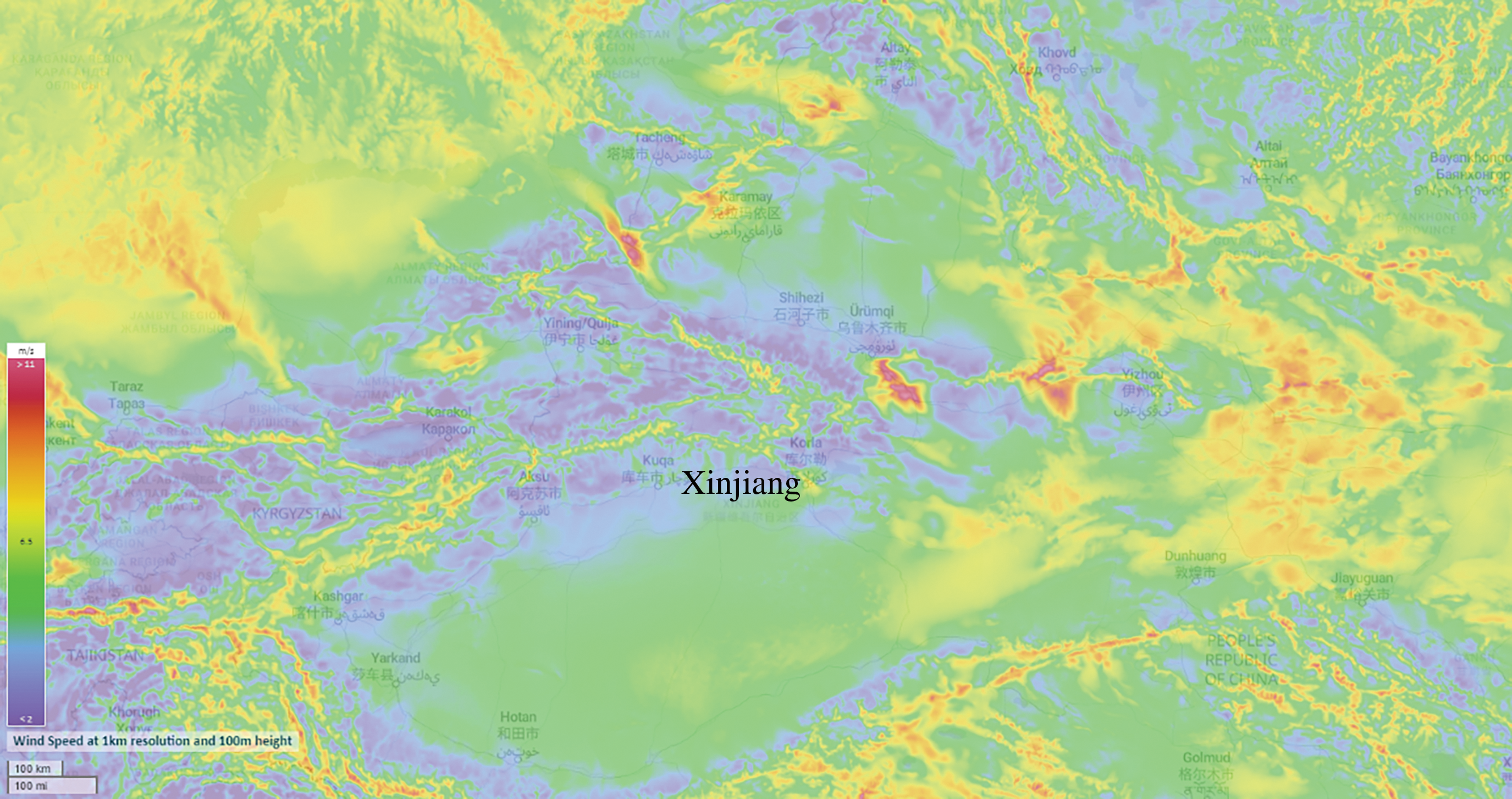
Figure 1: Average wind speed at 100 m altitude in Xinjiang

The data studied in this paper is derived from an unpublished historical wind power dataset of four power stations within a wind farm in the Xinjiang region of China in 2019. Among these power stations, the installed capacity of power station #1, power station #2, and power station #3 is 201 MW each, while power station #4 has an installed capacity of 300 MW. At the same time, the data set contains 13 key local meteorological parameters, including wind speed, wind direction, temperature, air pressure, and humidity, as well as wind power data of each power station. All data are recorded at 15-min intervals, providing high-resolution time series information. To enable the model to better capture seasonal patterns and trends, the annual data of each power station in this paper is divided into four sub-datasets based on seasonal changes, reflecting the potential impact of different seasons on wind power generation. The first 98% of each sub-dataset is utilized as the model training data, while the remaining 2% is reserved for testing.

2.2 Outlier Detection

Abnormal data may occur during the data collection, and those data need to be processed [34,35]. In addition, wind power generation is uncertain and intermittent. It is difficult to define the specific distribution of power data. Therefore, due to the advantage of avoiding over-reliance on the risk of specific distribution patterns, a boxplot method is selected to accurately identify outlier values in the data through the interquartile range IQR. Wherein IQR refers to the interquartile distance, that is the distance between the upper and lower quartiles.

The box plot is a graph used to show the distribution of data, which can effectively detect outliers in the data. The box plot consists of five numerical points, namely, minimum, lower quartile Q1, median, upper quartile Q3 and maximum. If there are outliers in the data, then these outliers will be drawn as independent points, and away from other data points. Therefore, it can easily identify these outliers by observing the box plot because they do not conform to the distribution of normal data points. This is the principle of box plot detection of outliers.

When using a boxplot for outlier detection, the threshold range of outliers is usually determined according to the IQR. If a value is less than the lower limit (Q1−1.5×IQR) or greater than the upper limit (Q3+1.5×IQR), it is considered an outlier.

Subsequently, the detected outliers are replaced with missing values, and then the missing values are uniformly processed.

2.3 Rectification of Missing Values

There are several ways to deal with the missing values in the data set, including direct deletion, special value interpolation, dummy variable, mean value filling, and regression filling. The direct deletion method is simple and easy to operate, but it has a great negative impact on the later data analysis. Given the type of data set in this paper, neither the dummy variable method nor the regression filling method is applicable. Considering the continuity of wind-related data, the mean filling method does not easily maintain the continuity of the data set, so the last observation carried forward method is selected to fill in the missing data.

2.4 Seasonal and Trend Decomposition Using LOESS

STL is a robust method for decomposing time series data Yt into trend Tt, seasonal St, and residual Rt components [36]. STL is highly desirable for time series decomposition due to its following advantages: first, it can handle any type of seasonality. Second, it can be easily adjusted by trend-cycle smoothening. Third, it is robust to outliers. Finally, it allows the seasonal component to change over time [37–39].

STL is an iterative regression algorithm, which consists of two internal and external cyclic mechanisms. The inner cycle mainly calculates trend components and seasonal components. The seasonal component is fitted by locally weighted regression and the trend component is obtained by a low-pass filtering algorithm. The outer loop is used to obtain the residual components, and the robustness weights are calculated in each loop to reduce the influence of outliers on the inner loop. The main steps of the inner loop are as follows:

(a)   Detrending. At iteration k+1 of the inner loop, remove the trend component obtained by the previous iteration, and get Ytdetrend=Yt−Tt(k);

(b)   Seasonal smoothing. Smooth the seasonal term which is denoted as Ct(k+1);

(c)   Low-pass filtering of the smoothed seasonality. The result sequence of the previous step is processed by moving the average and obtaining the sequence Lt(k+1) using local weighted regression;

(d)   Detrending of the smoothed seasonality. Remove the smoothed seasonal item sub-series as St(k+1)=Ct(k+1)−Lt(k+1);

(e)   Deseasonalizing. Remove seasonal items and subtract the seasonal component Ytdeseason=Yt−St(k+1);

(f)   Trend smoothing. Smooth the data after removing the seasonal term and trend term. Obtain the trend component Tt(K+1) by local weighted regression.

In the outer loop, residual component Rt is calculate as Rt(k+1)=Yt−St(k+1)−Tt(k+1). Where the large values in Rt are considered outliers and their weights are calculated. In the subsequent inner loop iteration, these weights are utilized to reduce the impact of anomalies detected in the previous iteration of the outer loop.

Time series decomposition models are divided into additive and multiplicative models. Since the wind power curve mostly shows a seasonal pattern with a period of one day, the additive time series decomposition method is chosen over the multiplicative time series decomposition in this paper. The flow of the STL algorithm is shown in the Fig. 2.

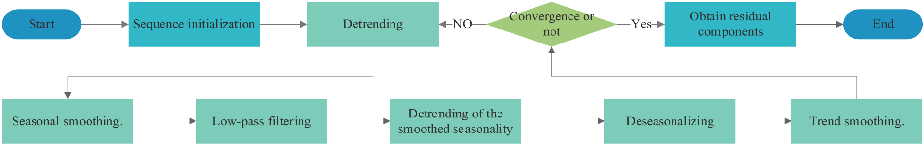
Figure 2: Flowchart of STL algorithm

3  STL-IAOA-iTransformer Forecast Model

In this section, IAOA will be introduced and the iTransformer model optimized by IAOA will be presented.

3.1 Improved Arithmetic Optimization Algorithm

3.1.1 Arithmetic Optimization Algorithm

AOA is inspired by the four mixed operations in arithmetic [31]. The algorithm selects an optimization strategy through a mathematical function accelerator and divides the whole process into exploration and development. That is, global exploration by multiplication, and division operation and local development by addition and subtraction operation [31,40]. The specific steps of AOA are as follows:

(a)   AOA generates a uniformly distributed random population. The initial population can be obtained by the following formula:

Oi,j=Rand×(Ub−Lb)+Lb(1)

    where Ub is the upper bound value of particle position, Lb is the lower bound value of particle position, Rand is the random number between [0, 1], and Oi,j is the position of the ith solution in the j dimensional space.

    Judging from the value of math optimizer accelerated (MOA) function and retrograde global search or local development:

MOAt=Min+(Max−Min)×a(2)

a=t/T(3)

    where MOAt is the current value of accelerator function, Min is the minimum value of the acceleration function and Max is the maximum value of the acceleration function, respectively; a is the linear convergence factor; t is the current number of iterations; T is the maximum number of iterations. When r1<MOAt, r1 is the random number between [0, 1], the function will enter the global exploration stage, otherwise, it will enter the local development stage.

(b)   Multiplication or division strategies are chosen based on the random number r2. These two strategies have high discretization, which is conductive to the exploration of the example in the algorithm space. The calculation formula is as follows:

O(t+1)={Ob(t)÷(MOP+ε)×((Ub−Lb)×μ+Lb),r2<0.5Ob(t)×MOP×((Ub−Lb)×μ+Lb), otherwise(4)

    where r2 is the random number between [0, 1]; O(t+1) is the position of the next generation particle; Ob(t) is the position of the particle with the best fitness at present; μ is the control coefficient of the search process; ε is a small integer number; MOP is the probability of the mathematical optimizer, which is calculated as follows:

MOP(t)=1−(a)1α(5)

    where MOP(t) is the probability of the current mathematical optimizer; α is the iterative sensitivity coefficient, and the higher value, the greater the influence of the number of iterations on MOP(t).

(c)   Finally, AOA is developed locally by addition strategy and subtraction strategy. Both of these strategies have significant low dispersion and can easily approach the target, which accelerate the process of finding the optimal solution, as

O(t+1)={Ob(t)−MOP×((Ub−Lb)×μ+Lb),r3<0.5Ob(t)+MOP×((Ub−Lb)×μ+Lb), otherwise(6)

    where r3 is a random number between [0, 1].

3.1.2 Improved Arithmetic Optimization Algorithm

In AOA, MOA and MOP are used to adjust global search and local search, respectively. It can be seen from Eqs. (2) and (6) that both MOA and MOP change with the linear convergence factor a. So, the transformation of search and utilization ability of MOA and MOP depends on a in the optimization process. It can be seen from Eq. (3) that with the continuous increase of iteration number, a will gradually increase to 1 linearly. However, the optimization process of MOA and MOP is complicated and changes non-linearly, so the linear update strategy of a cannot fully reflect the actual conditions of the optimization process of MOA and MOP. To address this, this study introduces nonlinear convergence factor b whose formula is as follows:

b=sin⁡(ηtTπ+φ)(7)

where η and φ are relevant parameters.

At this point, the MOA and MOP can be updated as follows:

MOAt′=Min+(Max−Min)×b(8)

MOP′(t)=1−(b)1α(9)

When AOA is locally developed in the later period, the convergence accuracy will gradually become low and it is easy to fall into the local optimal solution. At this point, in order to improve the convergence accuracy and make the algorithm jump out of the local optimum, the adaptive weight strategy is adopted.

The mathematical expression of the adaptive adjustment of search strategy is as follows:

ω=1−et/T−1e−1(10)

O(t+1)=ω⋅Ob(t)÷(MOP′+ε)×((Ub−Lb)×μ+Lb)(11)

O(t+1)=ω⋅Ob(t)×MOP′×((Ub−Lb)×μ+Lb)(12)

O(t+1)=ω⋅Ob(t)−MOP′×((Ub−Lb)×μ+Lb)(13)

O(t+1)=ω⋅Ob(t)+MOP′×((Ub−Lb)×μ+Lb)(14)

Stochastic differential mutation strategy formulated as

O(t+1)=r1×(Ob(t)−O(t))+r2×(O′(t)−O(t))(15)

where O′(t) is a random individual in population.

In order to speed up the convergence and prevent the population from falling into the local optimum, each individual will update its position twice in each location updating process. Firstly, the first position update is carried out according to the original AOA, and then, the second position update is carried out according to the adaptive weight to obtain the best position before and after its change. These two strategies complement each other and improve the ability of the algorithm to find the optimal solution.

In summary, the following improvements are made to AOA:

(a)   Form an initial population, containing N randomly generated individuals, and initialize the parameters;

(b)   Initialize the population in the solution space, and set t = 1;

(c)   Make judgment, when t ≥ T, output the optimal solution; When t < T, the fitness of each individual is calculated and the optimal individual position is recorded;

(d)   Calculate the value of b according to Eq. (7), and update MOA and MOP according to Eqs. (8) and (9), respectively;

(e)   Randomly generate a value p within [0, 1]. Update the position of different individuals as follows;

(f)   According to Eq. (15), the population is perturbed by random differential variation, so that t = t + 1;

(g)   When the number of iterations is close to the predetermined maximum value, output the final optimization parameters; otherwise, return to step (b) and set t = t + 1.

The flow chart of IAOA is as follows (Fig. 3):

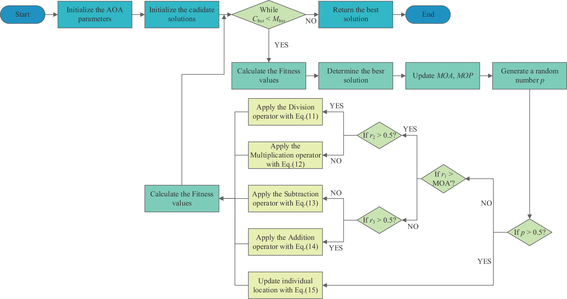
Figure 3: Flowchart of IAOA

3.2 iTransformer Model

In recent years, Transformer has shown its advantages in addressing time series prediction such as WPF [41]. Unlike deep learning techniques used to handle traditional sequential data, such as recurrent neural network (RNN) and LSTM, the Transformer model stands out for its unique feature of attention without recursion. In the context of supervised learning tasks like prediction, only the encoder component is pertinent. iTransformer is a variant of the traditional Transformer architecture. It addresses the problem of embedding multiple variables into a single time token. Instead, it embeds each variable of a time series independently as a variable token. This approach allows embedded tokens to better capture the global features of the time series and exploit the correlations between multiple variables more effectively.

3.2.1 Transformer Model Architecture

The main structure of the original Transformer is Encoder-Decoder architecture, supplemented by position coding, an ascending embedding layer, and a fully connected output layer. The schematic diagram is shown in Fig. 2. Due to its strong global information modeling capability, the Transformer is often used for long-period timing prediction problems.

Essentially, the self-attention mechanism is the information query mechanism [42]. Transformer’s multi-head attention mechanism processes input time series data into Query (Q), Key (K), and Value (V) by initially randomly setting WQ, WK, and WV weight matrices. Each attention can be given an output matrix Attention(Q,K,V). The self-attention mechanism can uncover relationships between values in a sequence and extract its global information. Its calculation formulas are shown in Eqs. (16) and (17):

Q=XWQ,K=XWK,V=XWV(16)

Attention(n)(Q,K,V)=Softmax(QKTdk)V(17)

where X is the input sequence; WQ, WK, and WV are the initialized weight matrices of Q, K, and V vectors, respectively. Softmax(⋅) is normalization calculation function; dk is the dimension of the input vectors K.

Each attention in Transformer is calculated in parallel to obtain output matrix Attention(n)(Q,K,V), and then the output result of the multi-head attention mechanism can be obtained by splicing and multiplying the corresponding weight matrix, as shown in Eq. (18).

output=Concat(Attention(n)(Q,K,V))Woutput(18)

where Concat(⋅) is output matrix concatenation function; Woutput is the weight matrix corresponding to the output matrix.

3.2.2 iTransformer Model’s Mechanism

In the realm of time series forecasting, traditional Transformer models often encounter issues of performance degradation and a surge in computational complexity, especially when dealing with sequences that have large lookback windows. Moreover, these models, when handling multivariate sequence predictions, frequently merge variables with different physical meanings into a single token, which may cause the predictive model to overlook the intrinsic correlations between variables. These limitations restrict the generalization capabilities of traditional Transformer models in time series forecasting tasks involving multiple input variables.

Conversely, the iTransformer model introduces an innovative solution that optimizes performance by overturning the structure of traditional Transformers. The iTransformer model abandons the complex encoder-decoder architecture found in traditional Transformer prediction models, retaining only the encoder component, which includes an embedding layer, a projector, and stackable transformer blocks, thereby making the model structure more concise and efficient. In this model, the feature embedding layer first independently maps the historical observation sequences of each variable to generate unique feature representations. Secondly, the self-attention mechanism is responsible for capturing the correlations between different variables. Then, the normalization layer ensures that the feature channels of all variables are in a similar distribution state, reducing the impact caused by the differences in the range of variable values. Lastly, the feed-forward network is responsible for extracting shared temporal features from historical observations and future predictions, transforming these features into forecast outputs. By maintaining the independence of variables, the iTransformer expands the model’s receptive field, making it perform more admirably in long-term sequence forecasting tasks. Overall, the comparison between traditional Transformer models and the iTransformer model can be visually presented through Fig. 4.

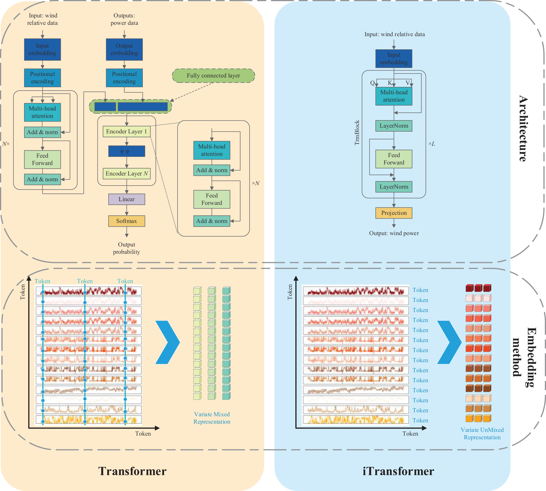
Figure 4: Comparison of transformer and iTransformer models

3.3 STL-IAOA-iTransformer Forecast Model

In this paper, a combined prediction model of STL-IAOA-iTransformer is used to conduct short-term WPF. Weather data such as wind speed and temperature are taken as input, and the wind power is taken as output. Firstly, the input data will be preprocessed to identify and handle outliers, and subsequently, the power data will be decomposed by STL, and multiple components obtained after decomposition will be used as the input of the prediction model. Secondly, all data will be input into the IAOA-iTransformer model for training, and the well-trained model will be used for actual power prediction. The prediction results of all components are obtained, and the final prediction results are obtained by superimposing all subsequences. The whole implementation process is shown in Fig. 5.

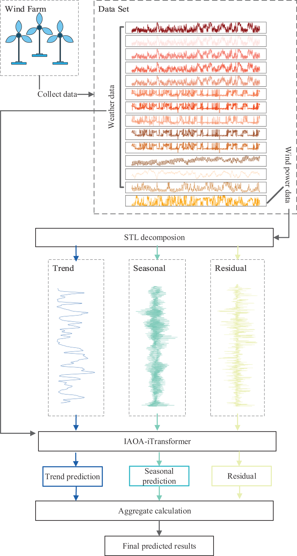
Figure 5: Flowchart of STL-IAOA-iTransformer algorithm

4  Case Studies

In this section, the STL-IAOA-iTransformer model proposed in this paper will be used to predict short-term wind power generation related to a wind farm in northwest China. The prediction results will be compared with other methods to verify the superiority of this method.

4.1 Model Evaluation Index

Root mean square error (RMSE) and mean absolute error (MAE) are used to measure the performance of each model. The indicators are calculated as follows:

RMSE=1n∑i=1n(y^i−yi)2,i=1,2,…,n(19)

MAE=1n∑i=1n|y^i−yi|,i=1,2,…,n(20)

where y^i and yi are the ith prediction value and true value, respectively. In short-term WPF, the smaller the two evaluation indicators, the more accurate the predicted result is.

The Diebold-Mariano (DM) test is commonly used to compare the forecasting results of two prediction models to determine which model provides better forecasts. The null hypothesis assumes that the two models have the same forecasting results, while the alternative hypothesis suggests that the forecasting results of the two models are different. When the significance level is set at 0.05, if the p-value is greater than 0.05, we fail to reject the null hypothesis, implying that the two models have the same effectiveness. If the p-value is less than 0.05, we reject the null hypothesis, indicating that the two models have different effects. When the null hypothesis holds, a DM test value greater than 0 indicates that Model 2 is superior to Model 1, while a DM test value less than 0 indicates that Model 1 is superior to Model 2.

4.2 Model Parameter Setting

In order to demonstrate the superiority of the proposed model, LSTM, back propagation neural network (BP), ELM, SVM, Transformer, iTransformer, SLT-transformer, AOA-transformer, and SLT-AOA-iTransformer algorithms are selected as comparative models. The simulations are conducted in Python. The model training ratio in the STL-IAOA-iTransformer combined model is 0.98. Besides, SimuNPS is applied to study the refined mathematical model of WPF. And the example of experimental environment configuration and hyperparameters configuration information are shown in Table 1.

4.3 Simulation Results and Analysis

This part will introduce and analyze the prediction results obtained by various methods in different seasons and different power stations.

4.3.1 STL Decomposition

Fig. 6 shows the decomposition results of STL for the wind power data of power station #1 in the spring of 2019. The first series shows the original series, the second series shows the trend component, the third series shows the seasonal component and the fourth series shows the loss component. As observed in Fig. 7, the seasonal component exhibits a high frequency of change and a seasonal change trend. The data at each moment is strongly correlated with changes in the previous period, which demonstrates long-term dependence. Considering the complex variation of seasonal components and the strong temporal correlation, the time-encoded IAOA-iTransformer model that can extract global information is selected for prediction.

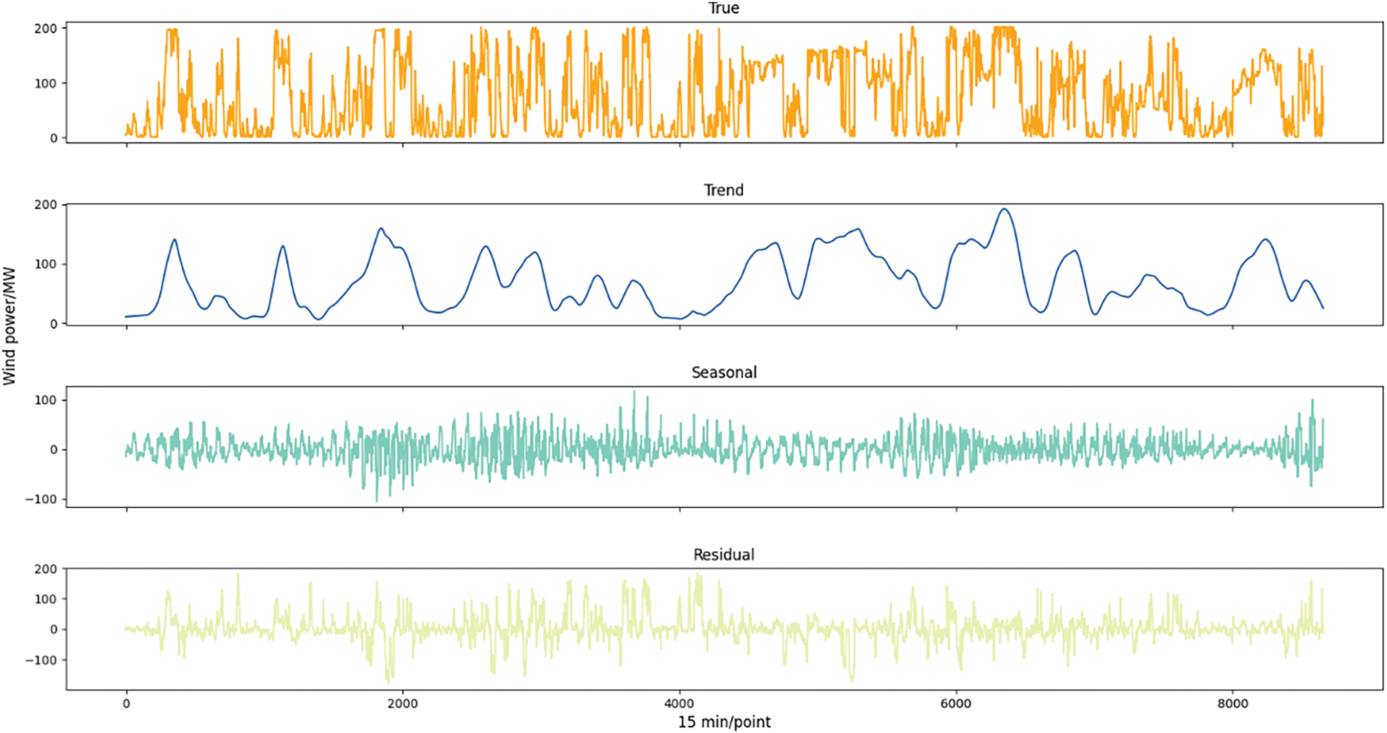
Figure 6: Results of STL decomposition (Take the data from spring 2019 as an example)

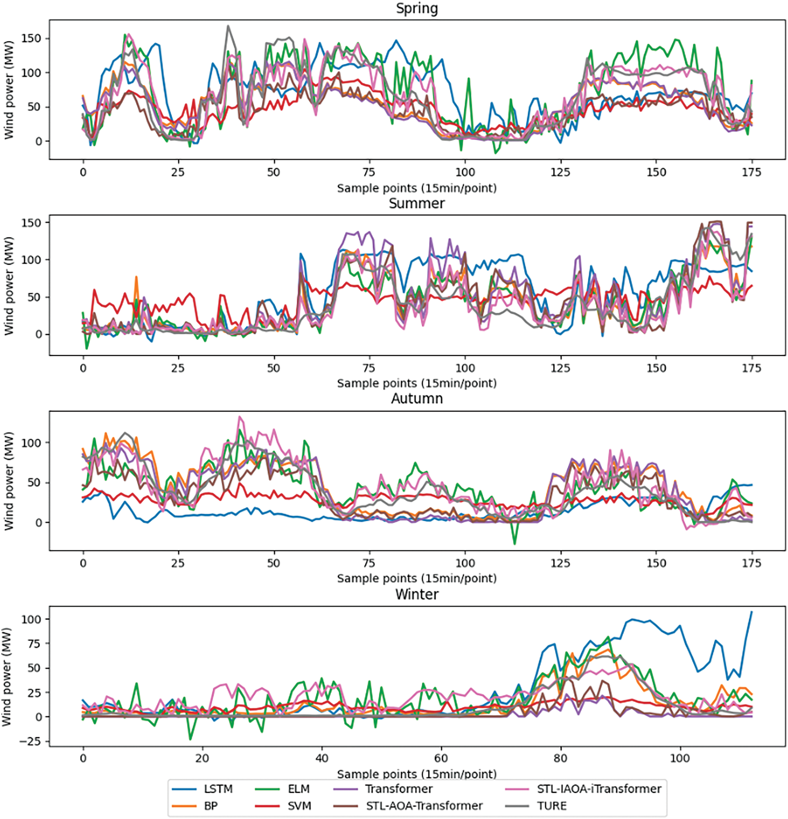
Figure 7: Comparison of prediction results of multiple algorithms in different seasons

4.3.2 Prediction Results under Different Seasons

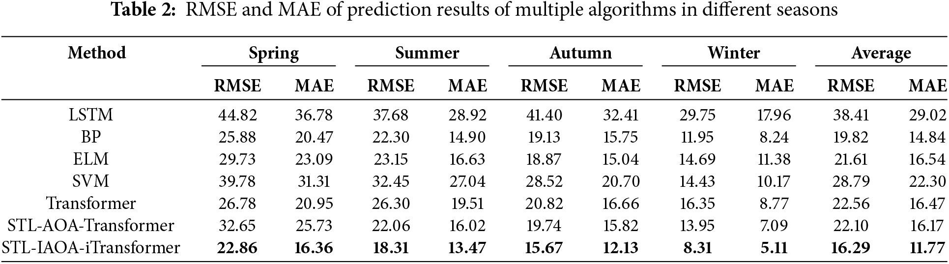
The annual historical power data of a wind farm in northeast China from January to December 2019 is selected for seasonal prediction. The STL decomposition analysis above shows that wind power output exhibits strong volatility and randomness with a notable seasonality. Based on the wind power generation data sets in different seasons, the STL-IAOA-iTransformer model and the other 6 models including LSTM, BP, ELM, SVM, Transformer, and STL-AOA-Transformer are selected to carry out prediction experiments respectively. The experimental results are shown in Fig. 7, and RMSE and MAE of prediction results of different algorithms in different seasons are shown in Fig. 8.

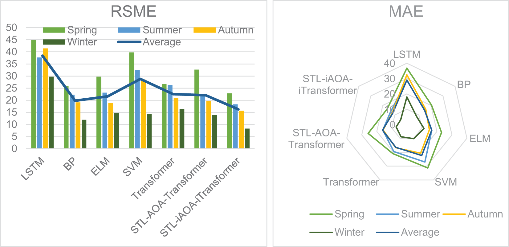
Figure 8: RMSE and MAE of prediction results of multiple algorithms in different seasons

It is evident from Figs. 7 and 8 that the test sequence displays fluctuating characteristics, suggesting that the actual wind sequence possesses nonlinear traits. All six prediction models can effectively capture the changing trend of the original wind power generation. Generally, there is a significant deviation between the prediction results obtained using the LSTM model and the actual wind power generations. The prediction results obtained by ELM, SVM, Transformer, and STL-AOA-Transformer models outperform those of the LSTM model. As illustrated in Fig. 7, the prediction curves of the STL-IAOA-iTransformer model and BP model closely align with the original wind power generation curve compared to other models. Furthermore, the prediction error results in Fig. 8 indicate that the prediction outcomes of the STL-IAOA-iTransformer model are notably superior to those of other models.

Table 2 demonstrates that the proposed algorithm STL-IAOA-iTransformer surpasses all other algorithms in terms of both RMSE and MAE measurements. For instance, the average RMSE of the proposed model is decreased by 57.60%, 17.80%, 24.63%, 43.44%, 27.81%, and 26.30% compared to LSTM, BP, ELM, SVM, Transformer, and STL-AOA-Transformer models, respectively. Similarly, the average MAE of the proposed model is decreased by 59.45%, 20.70%, 28.83%, 47.24%, 28.56%, and 27.20% compared to other algorithms. These findings suggest that the STL-IAOA-iTransformer algorithm exhibits a strong correlation between the predicted outcomes and the actual power curve.

4.3.3 Prediction Results under Different Power Stations

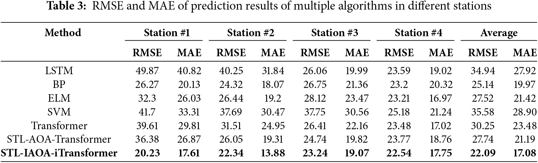
The historical power data of different power stations of a wind farm in Xinjiang from March to May 2019 in spring is selected to verify the performance of different models. The comparison of the predicted wind power and the real power of different prediction methods is shown in Fig. 9, and RMSE and MAE of prediction results of different algorithms in different seasons are shown in Fig. 10.

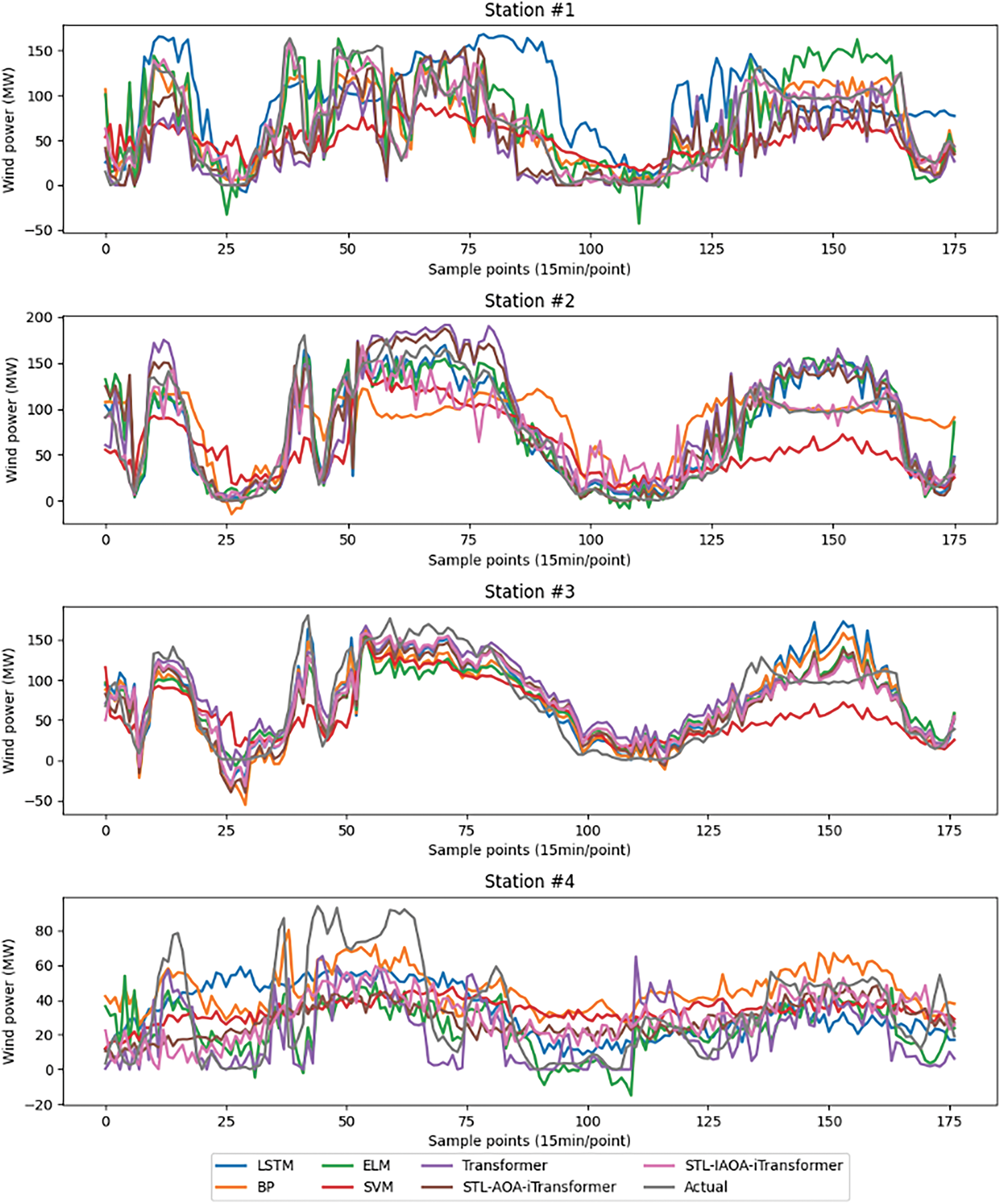
Figure 9: Comparison of prediction results of multiple algorithms in different power stations

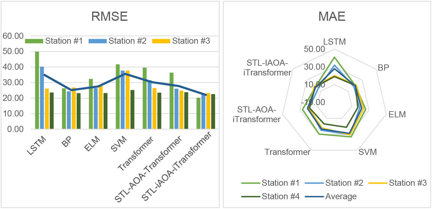
Figure 10: RMSE and MAE of prediction results of multiple algorithms in different stations

Based on the data presented in Fig. 9, it is evident that there is a certain regularity in the wind power output of various power stations during the same season. The proposed model in this study demonstrates both adaptability and superiority in accurately predicting power output across different locations. A visual inspection of Fig. 9 reveals that the STL-IAOA-iTransformer model closely aligns with actual wind power generation in simulation experiments conducted for different wind power stations. Furthermore, Fig. 10 illustrates that the RMSE and MAE of the STL-IAOA-iTransformer model are notably lower compared to other algorithms used for comparison, and the data in Table 3 also strongly confirms this conclusion. The results show that the average RMSE of the proposed model is decreased by 58.21%, 13.80%, 24.59%, 61.09%, 36.97%, and 25.57% compared to LSTM, BP, ELM, SVM, Transformer, and STL-AOA-Transformer models, respectively. Similarly, the average MAE of the proposed model is decreased by 63.47%, 16.93%, 25.41%, 69.20%, 37.52%, and 24.08% compared to these algorithms. Through this comprehensive analysis of short-term WPFs, it is evident that the algorithm proposed in this study outperforms other comparative methods.

4.3.4 Prediction Results under Different Power Locations

This paper selects Xinjiang, China, as the research subject, mainly based on two considerations. First, from an academic research perspective, Xinjiang is located in Northwest China and has distinct climatic characteristics, such as large diurnal temperature differences and dramatic wind speed variations. These features make Xinjiang a challenging object for wind power generation forecasting. In the field of wind power forecasting, Xinjiang’s unique climatic conditions provide abundant research materials, thus possessing high academic research value. Secondly, from an engineering practice perspective, Xinjiang is not only rich in wind resources but also has vast land and a sparse population, making it an important base for wind power generation in China, with many wind power stations built here. Wind power generation in Xinjiang is of great significance to the local energy structure and economic development. Therefore, improving the accuracy of wind power generation forecasting has practical application value in optimizing the allocation of wind power resources, reducing energy costs, and enhancing the stability of the power grid.

To verify the applicability and forecasting effectiveness of the methods proposed in this paper under different climatic conditions, this paper also selects data from a wind power station in a certain area of Southwest China as comparative test data for experiments. Such a choice helps to evaluate the universality and robustness of the proposed methods, as the climatic conditions in the Southwest region significantly differ from those in Xinjiang, which is crucial for verifying the generalization capability of the model.

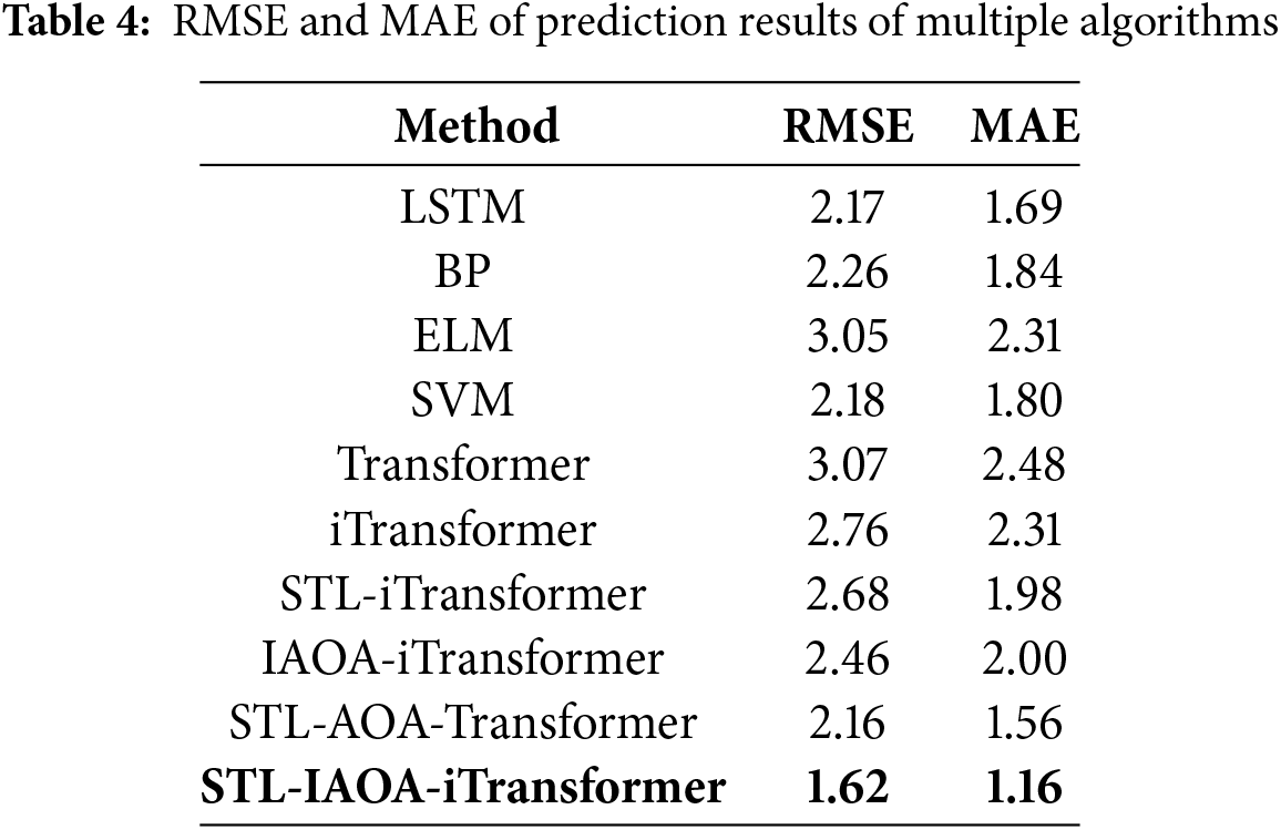
Fig. 11 shows the forecast result sequences of various algorithms in the experiment, and Table 4 presents the forecast errors of each algorithm. Table 4 lists the statistical data of forecast errors for different methods, which can quantitatively assess the performance of the forecasting models. From Table 4, it can be seen that the forecasting results of STL-IAOA-iTransformer are distinct from other algorithms and exhibit good performance. By comparing the STL-iTransformer model with the iTransformer model, it is evident that the RMSE and MAE of the STL-iTransformer model’s prediction results are both smaller than those of the iTransformer model. Therefore, it can be concluded that the model with STL decomposition has better predictive accuracy. The experimental results indicate that STL-IAOA-iTransformer has good universality.

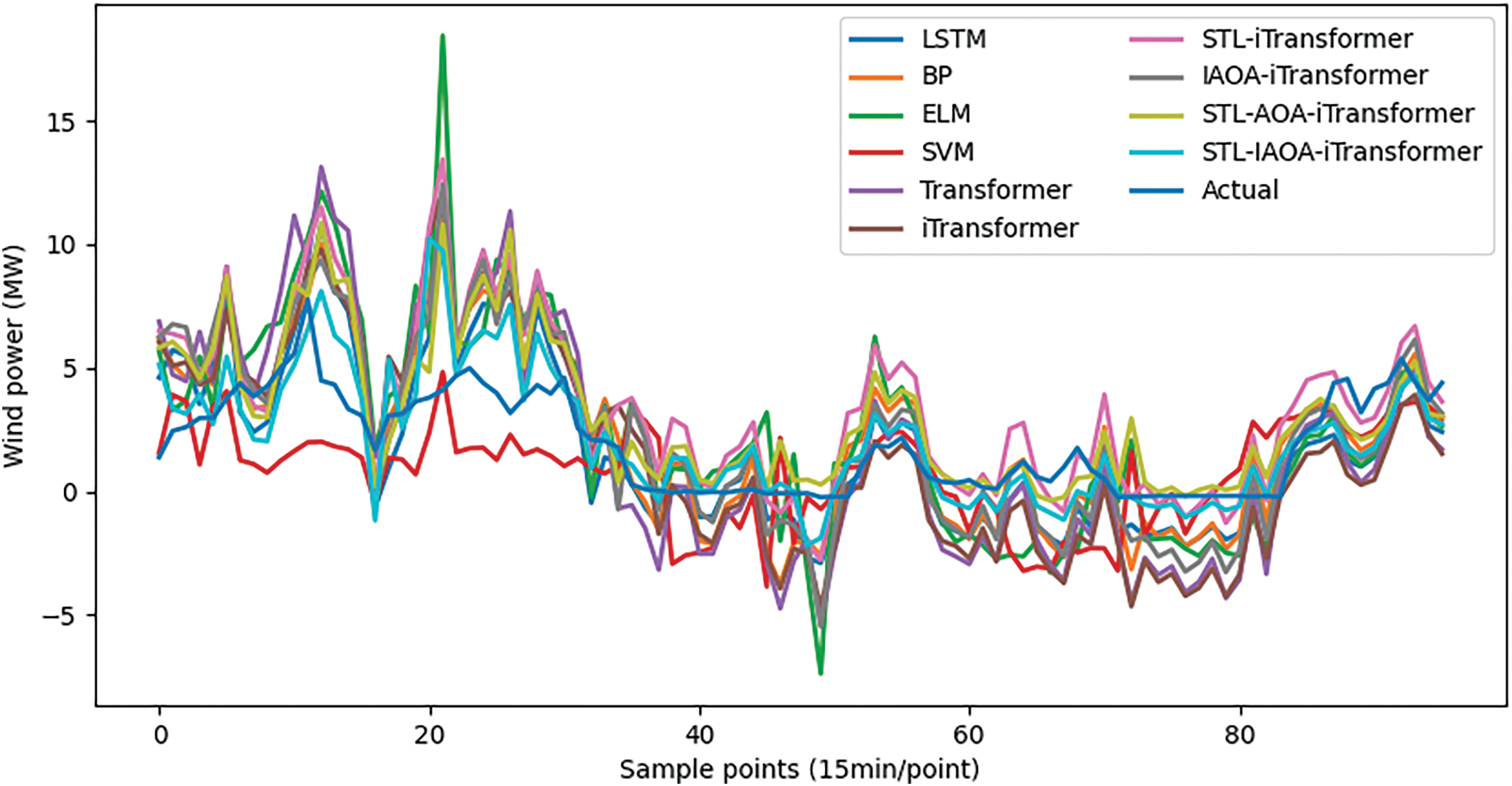
Figure 11: Comparison of prediction results of ablation experiment algorithms

4.3.5 Ablation Experiment

This study conducts ablation experiments to verify the roles of STL decomposition and IAOA in prediction, as well as to assess the improvements made to AOA. The experimental design for the ablation models is as follows:

(a)   Transformer: represents the basic Transformer model.

(b)   iTransformer: represents the basic iTransformer model, which does not include STL decomposition or IAOA.

(c)   STL-iTransformer: represents the model with STL decomposition added to the iTransformer.

(d)   IAOA-iTransformer: represents the model with IAOA added to the iTransformer.

(e)   STL-AOA-iTransformer: represents the model with both STL decomposition and AOA added to the iTransformer.

(f)   STL-IAOA-iTransformer: represents the model with both STL decomposition and IAOA added to the iTransformer.

Fig. 12 presents a comparison of the prediction results of ablation experimental algorithms across different seasons. The accuracy of wind power prediction conducted through ablation models is shown in Table 5. Table 5 displays the RMSE and MAE values for the proposed prediction model and the ablation models in predicting wind power data. In the ablation study, the average running time of the iTransformer was 23.1249 s. After applying STL decomposition, the average running time of STL-iTransformer was reduced to 22.3828 s. This not only decreased the computational time but also enhanced the predictive accuracy, demonstrating the necessity of STL decomposition.

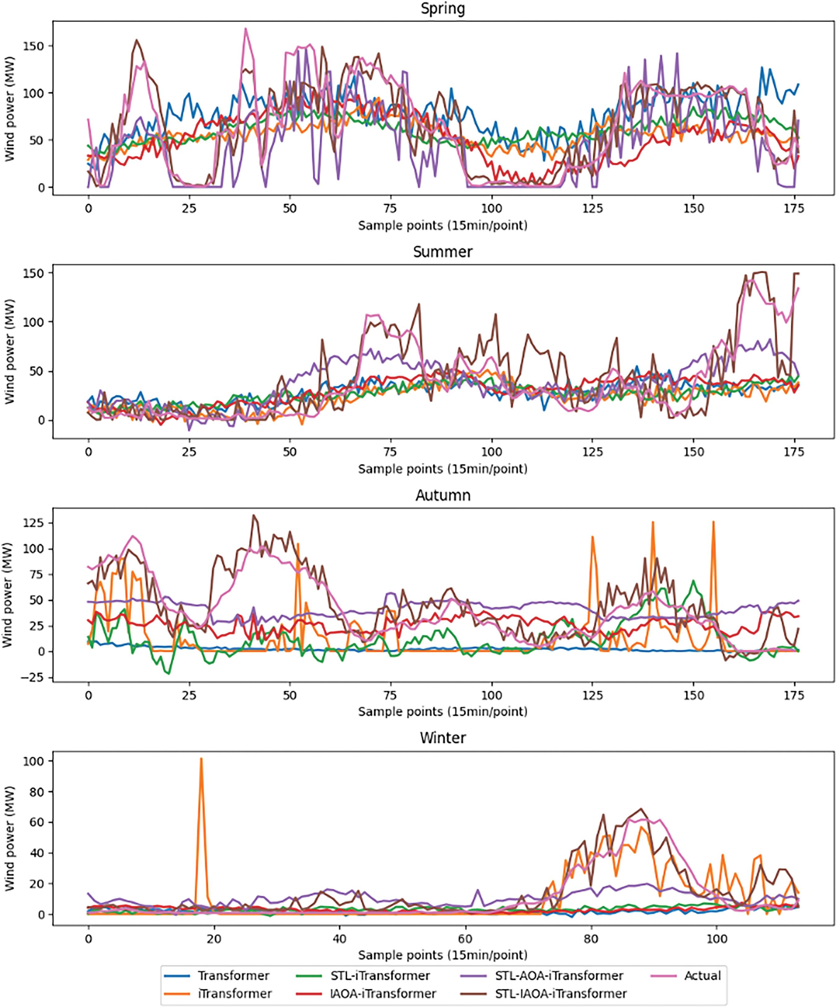
Figure 12: Comparison of prediction results of ablation experiment algorithms in different seasons

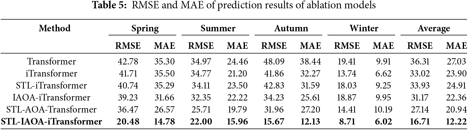
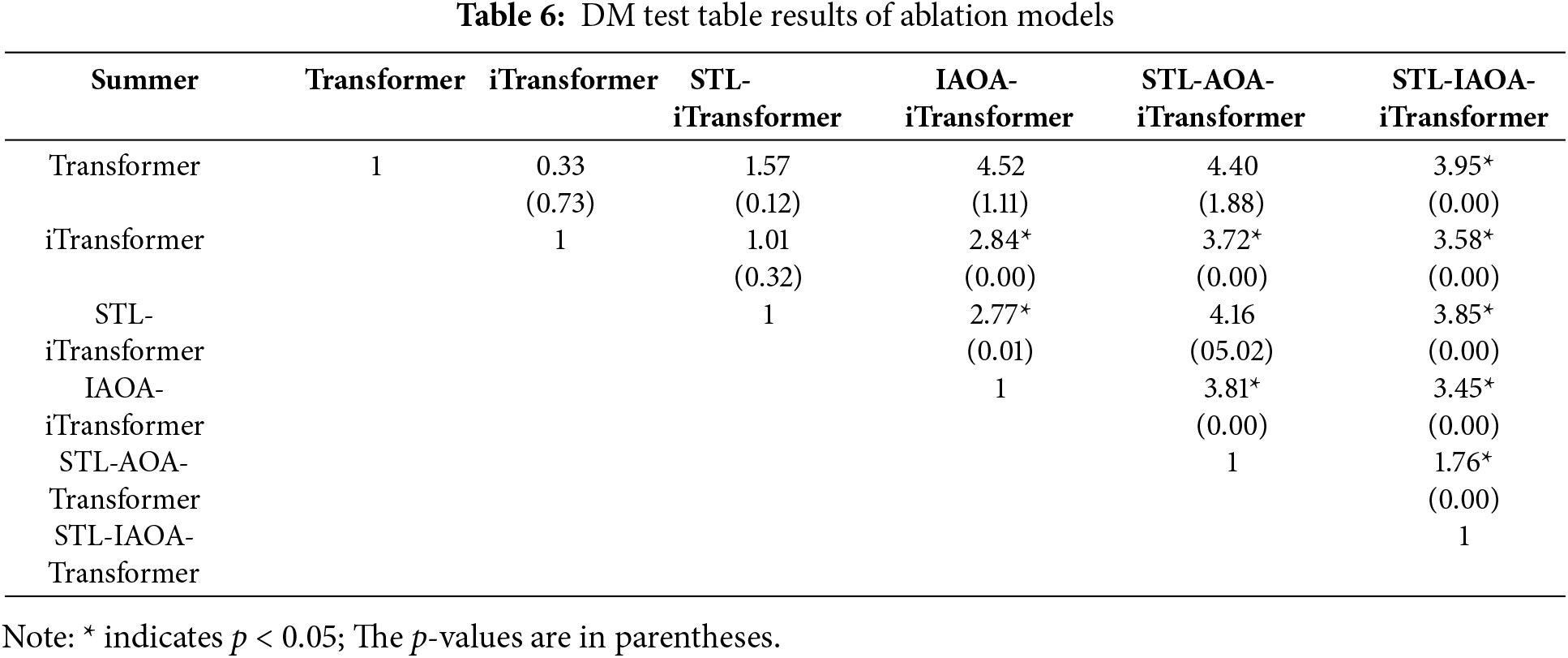
Table 6 presents the results of the DM test using the forecast outcomes of various algorithms in spring as an example. Taking the DM test results between STL-iTransformer and STL-AOA-iTransformer as an example, the p-value is less than 0.05, leading to the selection of the alternative hypothesis, which indicates that the two forecast sequences are not the same. The DM test value is greater than 0, suggesting that the forecast sequence of STL-AOA-iTransformer is closer to the actual sequence compared to that of STL-iTransformer, and thus has better predictive performance. The DM test reveals the superiority of STL-IAOA-iTransformer algorithm proposed in this paper.

4.3.6 Sensitivity Analysis of IAOA

A robust machine learning model often exhibits low sensitivity to parameters. Taking the spring data from power station #4 as an example, a parameter sensitivity test was conducted on the constructed IAOA using the control variable method, while keeping the other parameters, as well as the training and test datasets, unchanged. The selected sensitivity testing parameters include learning rate, epoch, α, and μ. These parameters were varied by ±20% to retrain and test the model, allowing us to compare any changes in testing accuracy, and the results are shown in Fig. 13. Overall, IAOA demonstrates relatively weak sensitivity to the aforementioned parameters. Even when these parameters fluctuate by ±20%, the MAE of the tests remains around 17 MW.

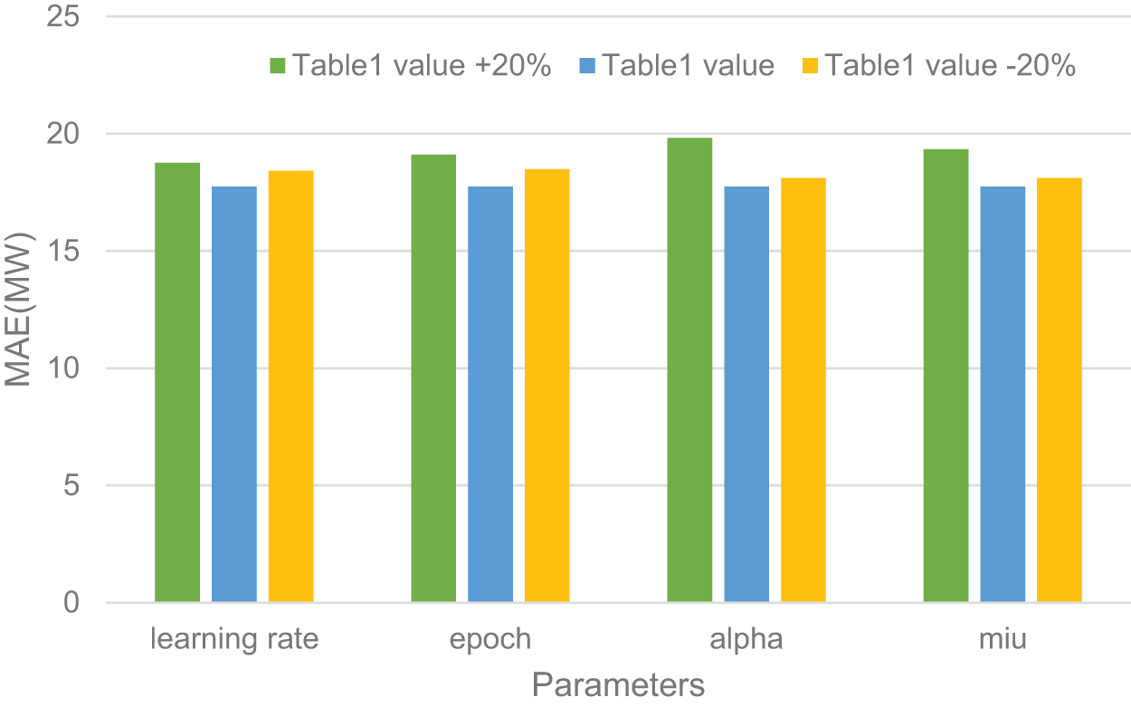
Figure 13: Comparison of test accuracy of STL-IAOA-iTransformer

5  Conclusions

To enhance the accuracy of short-term WPF, this study presents a hybrid power prediction model that combines data decomposition with the optimization of neural network algorithm hyperparameters using an improved heuristic algorithm. Moreover, to verify the effectiveness of the STL-IAOA-iTransformer model proposed in this paper, simulation experiments are carried out using the data of a wind power plant in Xinjiang, China, and the prediction results are compared with those of other state-of-art six comparison algorithms. The following conclusions are drawn through analysis:

(a)   The traditional AOA improved by nonlinear convergence factor, adaptive adjustment of the search strategy, and stochastic differential mutation strategy, can effectively avoid falling into local optimal value and achieve better optimization effect, and the stability of the IAOA algorithm has been verified through sensitivity analysis;

(b)   The STL-IAOA-iTransformer model proposed in this paper more effectively mines data characteristics and enhances prediction accuracy. Compared with other methods, the MAE of the proposed model decreased by 94.58%, 15.49%, 25.88%, 73.42%, 57.65%, and 44.30% on average in the forecast results of four different stations.

However, the model presented in this paper still has certain limitations. For instance, data requires preprocessing before prediction, and STL decomposition necessitates determining parameter settings through multiple attempts and domain knowledge. Therefore, the future work of this study can be summarized as follows:

(a)   Seasonal adjustment of algorithm parameters: Future studies could horizontally observe the prediction results of the same algorithm under different seasons to identify significant variations in prediction effects across seasons.

(b)   Simplification of meteorological information: Given the high complexity of meteorological information in both time and space, future research could focus on reducing the complexity of input data.

(c)   Integration of multiple data sources: WPF is influenced by a multitude of factors. Future work could involve the combination of various data sources, such as meteorological data, wind farm operational data, and geographic information data.

Acknowledgement: This work was supported by Yunnan Provincial Basic Research Project, National Natural Science Foundation of China, Yunnan Lancang-Mekong International Electric Power Technology Joint Laboratory and Major Science and Technology Projects in Yunnan Province.

Funding Statement: This work was supported by Yunnan Provincial Basic Research Project (202401AT070344, 202301AT070443), National Natural Science Foundation of China (62263014, 52207105), Yunnan Lancang-Mekong International Electric Power Technology Joint Laboratory (202203AP140001) and Major Science and Technology Projects in Yunnan Province (202402AG050006).

Author Contributions: The authors confirm contribution to the paper as follows: Formal analysis, methodology, software, validation, visualization, writing—original draft and writing—review & editing: Zhaowei Yang; Conceptualization, data curation, funding acquisition, methodology, project administration, supervision: Bo Yang; Methodology and project administration: Wenqi Liu; Software: Miwei Li; Formal analysis and software: Jiarong Wang; Funding acquisition and project administration: Lin Jiang; Funding acquisition and supervision: Yiyan Sang; Funding acquisition and writing—original draft: Zhenning Pan. All authors reviewed the results and approved the final version of the manuscript.

Availability of Data and Materials: The authors confirm that the data supporting the findings of this study are available within the article.

Ethics Approval: Not applicable.

Conflicts of Interest: The authors declare no conflicts of interest to report regarding the present study.

References

1. Jin J, Tian J, Yu M, Wu Y, Tang Y. A novel ultra-short-term wind speed prediction method based on dynamic adaptive continued fraction. Chaos Solitons Fractals. 2024;180(9):114532. doi:10.1016/j.chaos.2024.114532. [Google Scholar] [CrossRef]

2. Yang B, Zhong L, Wang J, Shu H, Zhang X, Yu T, et al. State-of-the-art one-stop handbook on wind forecasting technologies: an overview of classifications, methodologies, and analysis. J Clean Prod. 2021;283(6):124628. doi:10.1016/j.jclepro.2020.124628. [Google Scholar] [CrossRef]

3. Zhou G, Hu G, Zhang D, Zhang Y. A novel algorithm system for wind power prediction based on RANSAC data screening and Seq2Seq-Attention-BiGRU model. Energy. 2023;283(5):128986. doi:10.1016/j.energy.2023.128986. [Google Scholar] [CrossRef]

4. Rezaie H, Chung CH, Safari N. Ensemble wind power prediction interval with optimal reserve requirement. J Mod Power Syst Clean Energy. 2024;12(1):65–76. doi:10.35833/MPCE.2023.000464. [Google Scholar] [CrossRef]

5. Liao W, Wang S, Bak-Jensen B, Pillai JR, Yang Z, Liu K. Ultra-short-term interval prediction of wind power based on graph neural network and improved bootstrap technique. J Mod Power Syst Clean Energy. 2023;11(4):1100–14. doi:10.35833/MPCE.2022.000632. [Google Scholar] [CrossRef]

6. Fu X, Wu X, Zhang C, Fan S, Liu N. Planning of distributed renewable energy systems under uncertainty based on statistical machine learning. Prot Contr Mod Power Syst. 2022;7(4):1–27. doi:10.1186/s41601-022-00262-x. [Google Scholar] [CrossRef]

7. Xiao D, Chen H, Cai W, Wei C, Zhao Z. Integrated risk measurement and control for stochastic energy trading of a wind storage system in electricity markets. Prot Contr Mod Power Syst. 2023;8(4):1–11. doi:10.1186/s41601-023-00329-3. [Google Scholar] [CrossRef]

8. Tian LS, Yan X. Optimized prediction of short-term wind power intervals based on multiple data screening. Shandong Electr Power. 2024;51(5):38–46+62 (In Chinese). doi:10.20097/j.cnki.issn1007-9904.2024.05.005. [Google Scholar] [CrossRef]

9. Foley AM, Leahy PG, Marvuglia A, McKeogh EJ. Current methods and advances in forecasting of wind power generation. Renew Energy. 2012;37(1):1–8. doi:10.1016/j.renene.2011.05.033. [Google Scholar] [CrossRef]

10. Tang Z, Liu J, Ni J, Zhang J, Zeng P, Ren P, et al. Power prediction of wind farm considering the wake effect and its boundary layer compensation. Prot Contr Mod Power Syst. 2024;9(6):19–29. doi:10.23919/PCMP.2023.000221. [Google Scholar] [CrossRef]

11. Yang B, Zhu T, Cao P, Guo Z, Zeng C, Li D, et al. Classification and summarization of solar irradiance and power forecasting methods: a thorough review. CSEE J Power Energy Syst. 2023;9(3):978–95. doi:10.17775/CSEEJPES.2020.04930. [Google Scholar] [CrossRef]

12. Zhang C, Peng T, Nazir MS. A novel hybrid approach based on variational heteroscedastic Gaussian process regression for multi-step ahead wind speed forecasting. Int J Electr Power Energy Syst. 2022;136:107717. doi:10.1016/j.ijepes.2021.107717. [Google Scholar] [CrossRef]

13. Dong X, Wang D, Lu J, He X. A wind power forecasting model based on polynomial chaotic expansion and numerical weather prediction. Electr Power Syst Res. 2024;227(2):109983. doi:10.1016/j.epsr.2023.109983. [Google Scholar] [CrossRef]

14. Cassola F, Burlando M. Wind speed and wind energy forecast through Kalman filtering of Numerical Weather Prediction model output. Appl Energy. 2012;99:154–66. doi:10.1016/j.apenergy.2012.03.054. [Google Scholar] [CrossRef]

15. Yakoub G, Mathew S, Leal J. Direct and indirect short-term aggregated turbine- and farm-level wind power forecasts integrating several NWP sources. Heliyon. 2023;9(11):e21479. doi:10.1016/j.heliyon.2023.e21479. [Google Scholar] [PubMed] [CrossRef]

16. Zhang C, Zhou J, Li C, Fu W, Peng T. A compound structure of ELM based on feature selection and parameter optimization using hybrid backtracking search algorithm for wind speed forecasting. Energy Convers Manag. 2017;143(2):360–76. doi:10.1016/j.enconman.2017.04.007. [Google Scholar] [CrossRef]

17. Ouarda TBMJ, Charron C. Non-stationary statistical modelling of wind speed: a case study in Eastern Canada. Energy Convers Manag. 2021;236(9):114028. doi:10.1016/j.enconman.2021.114028. [Google Scholar] [CrossRef]

18. Carolin Mabel M, Fernandez E. Analysis of wind power generation and prediction using ANN: a case study. Renew Energy. 2008;33(5):986–92. doi:10.1016/j.renene.2007.06.013. [Google Scholar] [CrossRef]

19. Li J, Luo G, Hu W, Chen S, Liu X, Gao L. A SVM-based implicit stochastic joint scheduling method for ‘wind-photovoltaic-cascaded hydropower stations’ systems. Energy Rep. 2022;8(240):811–23. doi:10.1016/j.egyr.2022.10.273. [Google Scholar] [CrossRef]

20. Yu M, Niu D, Gao T, Wang K, Sun L, Li M, et al. A novel framework for ultra-short-term interval wind power prediction based on RF-WOA-VMD and BiGRU optimized by the attention mechanism. Energy. 2023;269(3):126738. doi:10.1016/j.energy.2023.126738. [Google Scholar] [CrossRef]

21. Sri Preethaa KR, Muthuramalingam A, Natarajan Y, Wadhwa G, Ali AAY. A comprehensive review on machine learning techniques for forecasting wind flow pattern. Sustainability. 2023;15(17):12914. doi:10.3390/su151712914. [Google Scholar] [CrossRef]

22. Ma J, Ma ZY, Ma HF. Wind power output prediction based on extreme learning machine. Comput Digit Eng. 2021;49(7):1465–8 (In Chinese). doi:10.3969/j.issn.1672-9722.2021.07.038. [Google Scholar] [CrossRef]

23. Abdel-Aty AH, Nisar KS, Alharbi WR, Owyed S, Alsharif MH. Boosting wind turbine performance with advanced smart power prediction: employing a hybrid ARMA-LSTM technique. Alex Eng J. 2024;96(1):58–71. doi:10.1016/j.aej.2024.03.078. [Google Scholar] [CrossRef]

24. Yu G, Liu C, Tang B, Chen R, Lu L, Cui C, et al. Short term wind power prediction for regional wind farms based on spatial-temporal characteristic distribution. Renew Energy. 2022;199(5):599–612. doi:10.1016/j.renene.2022.08.142. [Google Scholar] [CrossRef]

25. Chauhan S, Vashishtha G, Zimroz R, Kumar R. A crayfish optimised wavelet filter and its application to fault diagnosis of machine components. Int J Adv Manuf Technol. 2024;135(3):1825–37. doi:10.1007/s00170-024-14626-0. [Google Scholar] [CrossRef]

26. Ai C, He S, Hu H, Fan X, Wang W. Chaotic time series wind power interval prediction based on quadratic decomposition and intelligent optimization algorithm. Chaos Solitons Fractals. 2023;177(2):114222. doi:10.1016/j.chaos.2023.114222. [Google Scholar] [CrossRef]

27. Chen C, Li S, Wen M, Yu Z. Ultra-short term wind power prediction based on quadratic variational mode decomposition and multi-model fusion of deep learning. Comput Electr Eng. 2024;116(1):109157. doi:10.1016/j.compeleceng.2024.109157. [Google Scholar] [CrossRef]

28. Hanifi S, Cammarono A, Zare-Behtash H. Advanced hyperparameter optimization of deep learning models for wind power prediction. Renew Energy. 2024;221(15):119700. doi:10.1016/j.renene.2023.119700. [Google Scholar] [CrossRef]

29. He Y, Wang W, Li M, Wang Q. A short-term wind power prediction approach based on an improved dung beetle optimizer algorithm, variational modal decomposition, and deep learning. Comput Electr Eng. 2024;116(9):109182. doi:10.1016/j.compeleceng.2024.109182. [Google Scholar] [CrossRef]

30. Chen XH, Wu JK, Long YC, Wang ZP, Cai JJ. Short-term wind power prediction based on random forest optimized by kernel principal component analysis and carnivorous plant algorithm. Shandong Electr Power. 2024;51(1):59–67 (In Chinese). doi:10.20097/j.cnki.issn1007-9904.2024.01.007. [Google Scholar] [CrossRef]

31. Abualigah L, Diabat A, Mirjalili S, Abd Elaziz M, Gandomi AH. The arithmetic optimization algorithm. Comput Meth Appl Mech Eng. 2021;376(2):113609. doi:10.1016/j.cma.2020.113609. [Google Scholar] [CrossRef]

32. Cao W, Wang G, Liang X, Hu Z. A STAM-LSTM model for wind power prediction with feature selection. Energy. 2024;296(22):131030. doi:10.1016/j.energy.2024.131030. [Google Scholar] [CrossRef]

33. Cleveland RB, Cleveland WS, McRae JE, Terpenning I. STL: a seasonal-trend decomposition procedure based on loess. J Off Stat. 1990;6(1):3–33. [Google Scholar]

34. Ranjan KG, Prusty BR, Jena D. Review of preprocessing methods for univariate volatile time-series in power system applications. Electr Power Syst Res. 2021;191(4):106885. doi:10.1016/j.epsr.2020.106885. [Google Scholar] [CrossRef]

35. Chauhan S, Vashishtha G, Zimroz R. Analysing recent breakthroughs in fault diagnosis through sensor: a comprehensive overview. Comput Model Eng Sci. 2024;141(3):1983–2020. doi:10.32604/cmes.2024.055633. [Google Scholar] [CrossRef]

36. Da X, Ye D, Shen Y, Cheng P, Yao J, Wang D. A novel hybrid method for multi-step short-term 70 m wind speed prediction based on modal reconstruction and STL-VMD-BiLSTM. Atmos. 2024;15(8):1014. doi:10.3390/atmos15081014. [Google Scholar] [CrossRef]

37. Hyndman RJ, Athanasopoulos G. Forecasting: principles and practice. Melbourne: OTexts; 2018. [Google Scholar]

38. Tebong NK, Simo T, Takougang AN, Sandjon AT, Herve NP. Application of deep learning algorithms to confluent flow-rate forecast with multivariate decomposed variables. J Hydrol Reg Stud. 2023;46(15):101357. doi:10.1016/j.ejrh.2023.101357. [Google Scholar] [CrossRef]

39. Li S, Sun Y, Han Y, Alfarraj O, Tolba A, Sharma PK. A novel joint time-frequency spectrum resources sustainable risk prediction algorithm based on TFBRL network for the electromagnetic environment. Sustainability. 2023;15(6):4777. doi:10.3390/su15064777. [Google Scholar] [CrossRef]

40. Dhal KG, Sasmal B, Das A, Ray S, Rai R. A comprehensive survey on arithmetic optimization algorithm. Arch Comput Methods Eng. 2023;30(5):3379–404. doi:10.1007/s11831-023-09902-3. [Google Scholar] [PubMed] [CrossRef]

41. Mo S, Wang H, Li B, Xue Z, Fan S, Liu X. Powerformer: a temporal-based transformer model for wind power forecasting. Energy Rep. 2024;11(3):736–44. doi:10.1016/j.egyr.2023.12.030. [Google Scholar] [CrossRef]

42. Ghimire S, Nguyen-Huy T, AL-Musaylh MS, Deo RC, Casillas-Pérez D, Salcedo-Sanz S. Integrated Multi-Head Self-Attention Transformer model for electricity demand prediction incorporating local climate variables. Energy AI. 2023;14(2):100302. doi:10.1016/j.egyai.2023.100302. [Google Scholar] [CrossRef]