Flow and Heat Transfer Characteristics of Natural Gas Hydrate Riser Transportation

1  Introduction

In recent years, many countries have increasingly turned their attention to natural gas hydrates, driven by their abundant reserves and eco-friendly benefits [1,2]. Currently, there are two main methods for exploiting seabed natural gas hydrate (NGH). One method involves destabilizing the NGH by altering its stable conditions, leading to hydrate decomposition, and subsequently transporting the decomposed natural gas to the sea surface via thermal excitation, pressure reduction, chemical agents, and CO2 replacement [3–5]. The second method, involving the direct extraction of NGH, is known as the solid fluidization method [6,7]. This method pulverizes the hydrate into particles, performs a preliminary separation, and sieves the rocks and silt to remove the hydrate particles. The hydrate particles are then transported to the surface via risers using hydraulic lifting technology, where they are left to decompose at high temperatures and low surface pressures. Because hydrate slurries undergo phase transformations during transportation due to environmental changes, it is necessary to study the gas–liquid–solid three-phase flow of hydrates in pipelines [8]. This approach can not only prevent hydrate blocking in pipelines but also provide a design basis for hydraulic systems.

Research on hydrate grouting in vertical pipelines is important for hydrate solid-flow mining. However, its high cost poses a significant barrier to widespread adoption. In recent years, the progress in computational fluid dynamics (CFD) has enabled the utilization of CFD numerical simulation technology to address multi-phase flow in hydrate slurry tubes, effectively tackling the issues of high experimental cost and difficulty [9,10]. Balakin et al. [11,12] performed a CFD simulation study to investigate the deposition phenomenon of R11 hydrates in a turbulent pure water system. Fatnes [13] modeled the flow characteristics of a hydrate grout in a horizontal pipe using ANSYS CFX software. Jiang et al. [14] conducted an orthogonal simulation test to examine the impacts of hydrate grout velocity, hydrate particle size, and hydrate volume fraction on the flow characteristics of hydrate grout in a bend. Song et al. [15–18] developed a population phase equilibrium model to simulate the flow characteristics of R11 hydrate grout in horizontal tubes, encompassing phenomena such as accumulation, fragmentation, and deposition. Zhou et al. [19] conducted a finite difference iterative simulation to investigate the flow characteristics of hydrate grout in a vertical wellbore, focusing on variations in solid- and gas-phase contents. Liu et al. [20] employed the Euler multiphase flow model within a CFD framework, along with a finite-rate/eddy-dissipation model, to analyze the impact of the decomposition phenomenon of natural gas hydrate (NGH) slurry on the flow characteristics within a vertical pipe. Although these studies have significantly advanced the understanding of hydrate grout flow in vertical pipelines, several limitations remain. Specifically, the accumulation phenomena during flow have not been comprehensively addressed, nor have the interactions of various variables influencing hydrate grout flow been fully explored. These gaps necessitate further investigation and refinement.

Drawing upon the multi-phase flow characteristics of NGH in the development riser [21], this study utilized the aforementioned theory of flow and heat transfer characteristics, along with a population balance model [22], to simulate the flow and heat transfer behaviors of NGH within the riser. The group equilibrium model was applied to Fluent to simulate the flow state of hydrate in the development riser, the accumulation and fragmentation process of hydrate particles in the pipeline was studied, and the flow and heat transfer characteristics of hydrates in pipelines with different volume fractions and flow velocities were investigated.

2  Mathematical Model Establishment

The basic assumptions for modeling the gas hydrate development riser transportation process are as follows: (1) the fluid is an incompressible medium; (2) fluid particles are considered as continuous media; (3) the temperature of the fluid flow in the vertical pipe remains constant; and (4) during the analysis of heat transfer decomposition characteristics, the phase transformation of the hydrate is not taken into account, meaning that the phase mass transfer within the hydrate is disregarded.

2.1 Basic Governing Equations

In this study, the liquid-solid mixed phase was chosen as the focus of research for the turbulent flow of natural gas hydrate. The individual turbulent action effects of either the carrier phase or the solid phase were not isolated and considered separately throughout the entire flow process [23–26]. The selection of the turbulence model directly affects the accuracy of the flow field turbulence characteristic description and the difficulty of solving numerical equations [27]. The k-ω turbulence model, RNG (Re-normalization group) k-ε turbulence model, and Spalart–Allmaras turbulence model are generally used in numerical simulation. A comparison of these models is listed in Table 1.

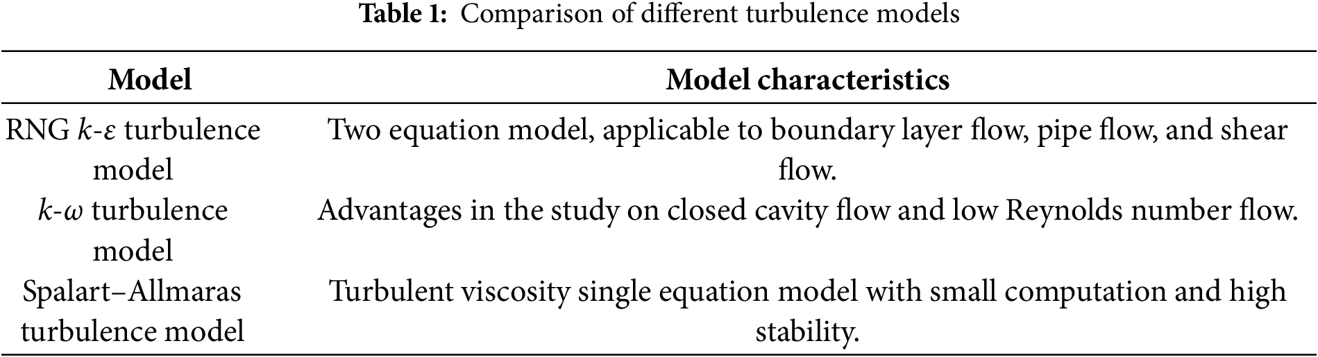
Comparing the three turbulence models, the RNG k-ε turbulence model was determined to be the most suitable for studying the hydrate flow characteristics in pipelines. This model introduces modifications to the turbulent viscosity and accounts for rotational flows as part of the averaged flow, making it particularly well-suited for handling flow in pipes with significant streamline curvature. Consequently, the RNG k-ε model was selected as the turbulence model for this study [28]. In this model, the equations for the turbulent kinetic energy (k) and the associated dissipation rate associated (ε) are reported in Eqs. (1)–(3):

∂∂t(ρmk)+∇.(ρmumk)=∇.(μt,mσk∇k)+Gk,m−ρmε(1)

∂∂t(ρmε)+∇.(ρmumε)=∇.(μt,mσε∇ε)+εk(C1Gk,m−C2ρmε)(2)

um=∑i=12αiρiui∑i=12αiρi(3)

The turbulent viscosity is expressed in Eq. (4):

μt,m=ρmCµk2ε(4)

The turbulent kinetic energy generated by the laminar velocity gradient is shown in Eq. (5):

Gk,m=μt,m(∇um+(∇um)T):∇um(5)

where k is kinetic energy, m2/s2; ε is dissipation rate, m2/s3; σk and σg are the turbulence numbers; C1 and C2 are constants, C1 = 1.42, C2 = 1.68.

2.2 Multiphase Flow Model and Turbulence Model

The Euler–Euler two-fluid model was employed to simulate the hydrate multiphase flow model, compromising momentum, continuity, and constitutive closed equations.

The continuity equation is shown in Eq. (6):

∂(ρiαi)∂t+∇⋅(ρiαiui)=0(6)

The momentum equation is shown in Eq. (7):

∂(ρiαiui)∂t+∇⋅(ρiαiuiui)=−αi∇p+αiρig+∇⋅τi+Mi(7)

where i is aqueous phase or hydrate particles; t is time, s; ρ is density, kg/m3; α is volume fraction; ∇ is Laplacian operator; p is pressure, Pa; Mi is the momentum exchange term between phases, kg/(m·s)2.

Fluent software was used to simulate the momentum exchange between phases in multiphase flow, with special consideration given to the drag force, comprising shape resistance and friction resistance, which was calculated using the Gidaspow model between the phases [29].

Using the Wen-Yu formula shown in Eq. (8) to calculate:

β=34CD(1−φs)φsρ1|v1⇀−vs⇀|dp(1−φs)−2.65(8)

Using the Ergun formula shown in Eq. (9) to calculate:

β=150φs2μ1(1−φs)dp2+74φsρ1|v1⇀−vs⇀|dp(9)

The drag force between phases can be calculated by Eq. (10):

FD⇀=β⋅vr⇀(10)

Standard settings of turbulent kinetic energy (k) and dissipation rate (ε) are adopted in Fluent simulation, and the near-wall surface is processed by standard wall function.

2.3 Population Balance Model

The population balance model is an effective method for combining macroscopic parameters with the microscopic behavior of bubbles [30–32]. The core of the population balance model lies in monitoring and tracking alterations in the quantitative density function of discrete phases, including particles, droplets, bubbles, and impurities, within the hydration flow of the development riser. This model establishes correlations between microscopic behaviors, such as nucleation, growth, aggregation, and fragmentation of discrete phase hydrates, and macroscopic characteristics like particle size, area, and volume of hydrates. It aims to preserve the microscopic properties of these discrete phase hydrates, represent the average movement of the continuous phase, and enhance the efficiency of calculations by optimizing the computational load.

The population balance model was introduced and applied as shown in Eq. (11) [33]:

dn(L,t)dt=12∫0Lαβ(L−L′,L′)n(L−L′,t)n(L′,t)dL′−n(L,t)∫0∞αβ(L,L′)n(L′,t)dL′+∫0∞b(L|L′)S(L′)n(L′,t)dL′−S(L)n(L,t)(11)

where n(L, t) represents the quantity density of hydrate particles at time t, 1/m3; β(L-L′, L′) respectively represents the collision frequency of hydrate particles with particle sizes of L-L′ and L′, m3/s; α is the coalescence efficiency of two hydrate particles after collision; S(L′) represents the crushing frequency of L′ hydrate particles, 1/s; b(L|L′) represents the probability that the hydrate particle size of L′ generates the hydrate particle size of L after L′ is broken.

The calculation formulas for the key parameters were chosen based on the kinetics of hydrate particle aggregation.

When investigating the collision frequency, priority is given to collisions resulting from flow shear and differential settlement [34]. The practical collision frequency of the hydrate particles was determined from the sum of the collision frequencies generated by the flow shear and differential settlement using the camp formula shown in Eq. (12) was adopted to calculate the collision frequency of differential settlement.

βDS=π4(Li+Lj)2|vi⇀−vj⇀|(12)

The settlement rate was calculated using Eq. (13):

V=347.56L1.54(13)

When the scale of the flow shear collision frequency exceeds that of the hydrate particles, the particles flow within the turbulent dissipation region. In this region, the local shear force within the vortices influences the aggregation behavior of the hydrates. At this stage, the formula for calculating the collision frequency of the hydrate particles is provided by Eq. (14):

βTH=8π15G(Li+Lj)38(14)

However, when the hydrate particles surpass the specified scale range, their flow enters the turbulent inertial region, where the hydrate flow is influenced by the mainstream field. At this point, the collision frequency of the hydrate particles was computed using Eq. (15) [35]:

βTG=23/2π(Li+Lj)34(ui2+uj2)2(15)

Because the continuous phase of the hydrate flow distribution in the development riser was water, there was no liquid-bridging force between the hydrate particles. The ratio of the fan flow shear force to the van der Waals force was mainly considered when calculating the coalescence efficiency of the hydrate particles using a curve model. The coalescence efficiency was calculated using Eq. (16):

α=z(H36πμ1GR3)0.18(16)

The crushing frequency calculation mainly considers the crushing caused by the flow shear, and the specific calculation formula is shown in Eq. (17):

S=EGmL,(17)

where E is the empirical constant.

In terms of the distribution function of particle size, a binary distribution is used as the distribution function of the fractured hydrate particle size, as shown in Eq. (18) [36]:

b(L|L′)={2L=12L′0L≠12L′(18)

Based on the above calculations of hydrate particle aggregation dynamics, Eqs. (12)–(18), the UDF (User-Defined Functions) is compiled to calculate the key parameters in the population balance model. The Lehr model of Fluent 15.0 software was used to simulate the hydrate particle breakage effect.

2.4 Heat Transfer Decomposition Model

The change in pressure and temperature during the flow of natural gas hydrate in the development riser leads to heat transfer decomposition of the NGH. The key is to solve for the decomposition mass source term (Sm) and energy source term (Sh).

Based on gas molecular dynamics theory, the molecular flow per unit area per unit time is given by Eq. (19) [37]:

mn=14Nv¯,(19)

where v¯ is the average molecular velocity; N is the number of molecules per unit volume; mn is the molecular flow, 1/(m2·s). According to the ideal gas equation of state, N can be obtained as shown in Eq. (20):

N=pkcT,(20)

where kc is the Boltzmann constant.

The probability distribution function Maxwell Boltzman [38] is used to calculate v¯, as shown in Eq. (21):

v¯=∫0∞vf(v)dv=8kcTπM(21)

where M is the molecular mass.

Eq. (22) can be obtained by substituting Eqs. (21) and (20) into Eq. (19), which is the Kundsen equation [39,40]:

mn=p2πMkcT(22)

The net evaporation of the gas-liquid interface is the molecular weight of the vapor escaping in the liquid phase minus the number of condensing molecules in the gas phase, and is calculated as shown in Eq. (23):

mn=12πMkc(plTl−pvTv)(23)

where Tl and Tv are the temperatures on the gas and liquid sides of the gas-liquid interface (K), respectively; pl and pv are the liquid and gas phase pressures, respectively (Pa). By comparison with the experimental values, it was found that the evaporation and condensation correction coefficient σc should be introduced for correction. The modified formula is shown in Eq. (24):

mn=2σc2−σc12πMkc(plTl−pvTv)(24)

The vapor–liquid interface evaporation mass flow is expressed by Eq. (25):

J=mn.M=2σc2−σcM2πkc(plTl−pvTv)(25)

where J is the mass flow rate of evaporation at the gas-liquid interface, kg/(m2·s), namely the hertz-Kundsen heat transfer decomposition model.

When the two gas–liquid phases are in equilibrium, the Clausius–Clapeyron equation [33] shows that the saturation gasification curve can be calculated, as shown in Eq. (26):

dpdT=ΔHT(1ρv−1ρL)(26)

where ΔH denotes the latent heat (J/kg). When it is close to saturation, the following equation can be obtained as shown in Eq. (27):

p−psat=ΔHT(1ρv−1ρL)(T−Tsat)(27)

Substituting Eq. (26) into Eq. (15), we obtain Eq. (28):

J=2σc2−σcM2πkcTsatΔH(1ρv−1ρl)T−TsatTsat(28)

Because the gas-liquid mass transfer is introduced through the source term in the mass equation, the above formula is multiplied by the gas-liquid interface area Al in the unit and divided by the unit volume Vcell, and both satisfy. As shown in Eq. (29):

AlVcell=6αid(29)

where αi is the volume fraction of phase i and d is the mean diameter of the spherical droplet (m).

Therefore, the mass source term in the mass conservation equation is shown in Eq. (30):

Sm=6αid2σc2−σcM2πkcTsatΔH(1ρv−1ρl)T−TsatTsat(30)

where Sm is the source term of decomposition quality, kg/(m3.s).

Define the coefficient β as Eq. (31):

β=6d2σc2−σcM2πkcTsatρvΔH(ρl−ρv)(31)

Finishing available as Eq. (32):

Sm=βαiρiT−TsatTsat(32)

where β is the relaxation factor of mass transfer time, s−1. Factors controlling decomposition intensity have different values in different research problems. Based on the above analysis, the hydrate flow heat transfer model studied in this chapter is summarized as follows:

When it is an evaporation process (Tl > Tsat), the liquid mass source term, gas mass source term, energy source term are shown as Eqs. (33)–(35):

Sm=−β∗alρl(Tl−Tsat)Tsat(33)

Sm=β∗alρl(Tl−Tsat)Tsat(34)

Sh=−β⋅alρl(Tl−Tsat)Tsat⋅ΔHevap(35)

When it is a condensation process (Tl < Tsat), the liquid mass source term, gas mass source term, energy source term are shown as Eqs. (36)–(38):

Sm=−β∗alρl(Tl−Tsat)Tsat(36)

Sm=β∗alρl(Tl−Tsat)Tsat(37)

Sh=−β⋅alρl(Tl−Tsat)Tsat⋅ΔHevap(38)

Herein, a1 is the liquid phase fraction; av is the gas phase fraction; ρl is the liquid density of the hydrate, kg/m3; ρv is the gas phase density of the hydrate, kg/m3; ΔH is the latent heat of condensation (J/kg); and ΔHevap is the latent heat of evaporation (J/kg).

When the pressure of the hydrate increased, the saturation temperature also increased. Based on the thermodynamic properties, the saturation temperature of the hydrate is positively correlated with the saturated vapor pressure. While the saturation temperature of the hydrate increases, the latent heat of vaporization decreases, and the latent heat of vaporization is negatively correlated with the saturation temperature. Using quadratic polynomial fitting as shown in Eqs. (39) and (40):

T=−4.40E−11P2+8.36E−05P+1.05E02(39)

H=6.48E−11T2−1.68E−04T+5.25E02(40)

Considering the influences of the saturation temperature, pressure, and latent heat of vaporization, Eqs. (33)–(40) were embedded in the Fluent solver through user-defined functions of the UDF and programmed in the C language to solve the heat transfer decomposition process in the model.

3  Physical Model Establishment

3.1 Geometric Model

A geometric model was constructed based on a pipeline with a flow characteristic experiment in a gas hydrate development riser. A vertical pipeline with length L = 3.0 m and diameter D = 5.02 cm was constructed in the three-dimensional model. This geometric setting corresponds to the relevant experiments (pipe length L = 3.0 m and diameter D = 2 in). Parameters such as the inlet, outlet, pipe wall, and roughness of the experimental ring were used to study the hydrate flow law.

Meanwhile, to study the heat transfer law of the hydrate, the length L of the 3D model was extended to 200 m to compare the influence of the flow rate and temperature on the heat transfer law under the premise of ensuring a stable flow of hydrate in the pipeline.

3.2 Mesh Division

The constructed geometric model is meshed using a hexahedron. The inlet wall is partitioned in steps of 1 mm, and eight-layer grid encryption is used near the wall to deal with the boundary layer effect [41], 8-layer grid encryption is used at the near wall. The remaining areas were divided into grids with a step size of 1 mm. The grid division of the riser and the inner section of the pipeline during the development of the model is shown in Fig. 1.

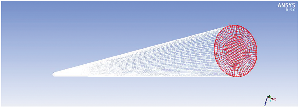
Figure 1: Effect drawing of the simulated pipeline

The pipe is divided into two sections, which not only reduces the error in the numerical simulation but also improves the efficiency of the grid operation. The origin of the 3D coordinate system of the calculation model was at the center of the circle of the entrance interface. The fluid medium was gas-liquid two-phase, the Y-axis was the flow direction, and the direction of gravity aligned with the negative direction of the Z-axis.

Compared to the laminar flow model, solving the turbulence model simulation depends more on mesh division, and it is necessary to divide an accurate mesh to achieve sufficiently accurate simulation results. The prediction of wall heat transfer and shear stress, and the development of flow medium separation have high requirements for near-wall treatment. The grid points of the first layer must be arranged outside the viscous bottom layer, and the grid space at the wall must meet the limit coefficient of 20 times the grid accuracy. Particularly in the case of a low-Reynolds-number flow, more attention should be paid to the spatial distance requirement of the grid near the wall. Because the boundary layer thins rapidly at low Reynolds numbers, if the grid near the wall is too sparse, the solution will diverge. Therefore, the key to hydrating turbulent flow is the numerical treatment of each governing equation near the wall surface, and scalar quantities, such as the average momentum, are mainly determined by the effective viscosity coefficient in space.

3.3 Grid Independence Verification

When the flow of solid fluidized hydrates was simulated using Fluent, the grid was comprised of approximately 1 million cells. To avoid bad simulation conditions, the number of grids is too low, the grid quality is low, the simulation results do not easily converge, and the accuracy of the simulation results becomes worse. Dividing too many grids will lead to a huge amount of computation and a long operation time, which consumes too much memory. Therefore, under the same boundary conditions, grid structures with different numbers were created to verify the independence of the grid. Pipeline points (3.6, 24, and 36) are selected as grid-independent and time-step-independent monitoring points to verify the flow rate and particle distribution.

The effects of the quality and quantity of meshing on the accuracy of the calculation results and computer operation efficiency were verified. The changes in the velocity and particle distribution monitoring points for the three grid schemes are shown in Fig. 2. According to the results of the trial calculation, the number of grids was set to 1,868,373 to ensure the accuracy and efficiency of the calculation.

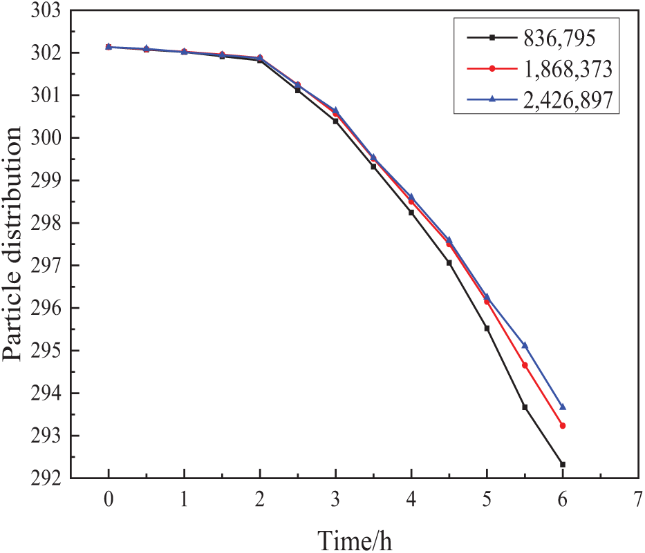
Figure 2: Flow velocity and particle distribution in different grid schemes

4  Numerical Simulation Method

4.1 Model Solution Settings

When using Fluent 15.0 software to solve the model, the parameters simulated in the model solution are listed in Table 2.

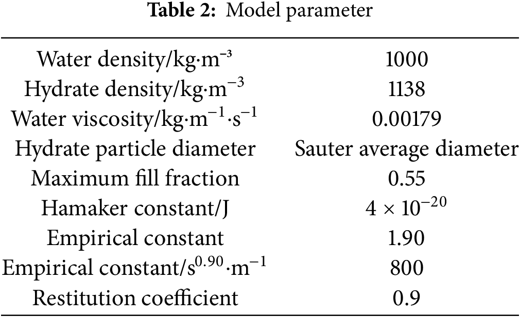
The inlet was set as a speed inlet, the outlet was set as a pressure outlet, the outlet pressure was 0 and the wall surface did not slip. Given that the hydrate’s flow direction opposes the gravity direction in the practical working conditions of the riser, the simulation accounts for this by reversing the gravity direction relative to the flow direction. A second-order upwind scheme was used for the simulation. When the residual of each factor converges to 10−5, it is considered that the residual of each factor converges, and the simulation ends.

4.2 Model Verification

Owing to the lack of hydrate flow experiments for riser development, the relevant experimental data are incomplete. To validate the accuracy of the model, the unit pressure drop was primarily used as the verification parameter, based on experiments detailed in the literature regarding the flow characteristics of hydrates in horizontal tubes. The working conditions of the validation model are listed in Table 3 and the results of the verification of the unit pressure drop are shown in Fig. 3. The results show that the model can simulate the hydrate flow more accurately.

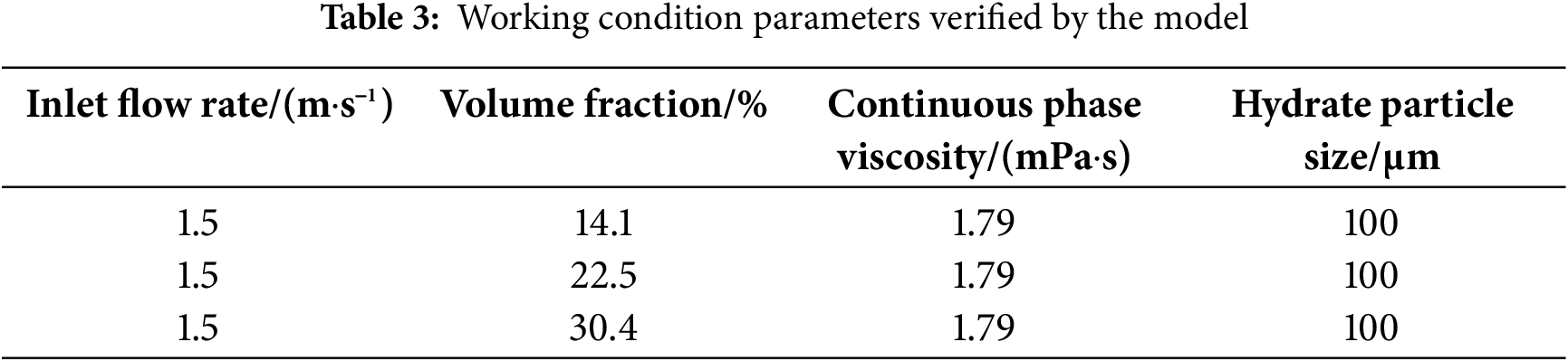
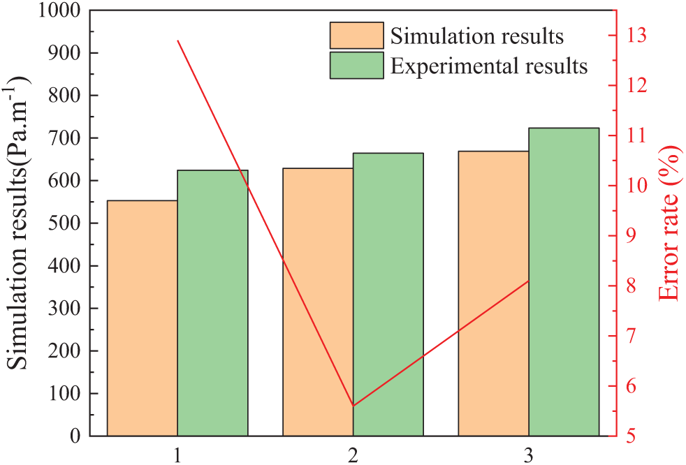
Figure 3: Verification results

4.3 Model Solution Strategy and Convergence Criteria

For complex flow problems, the first-order precision calculation strategy is generally adopted to calculate the initial flow field and improve the calculation accuracy such that calculation stability and higher calculation accuracy can be obtained. Regarding the relevant variables of the flow field, mass, momentum, and energy, there are first- and second-order precisions for solving the discrete element. If the flow-field variable does not change in the residual after many iterations, the calculation is considered to have completed the convergence of the discretization to determine the result.

They can be selected based on the complexity of the model, meshing form, and research objectives. The default calculation scheme with first-order accuracy converges easily; however, the dissipation is large, whereas the calculation result with second-order accuracy is more accurate and does not converge easily. To determine whether the simulation results meet the required calculation accuracy, it is necessary to observe the residual curve and often combine the changes in the relevant flow field variables. These are combined to determine whether the iteration meets the convergence standards.

5  Liquid Phase Dominated Flow Law in the Riser

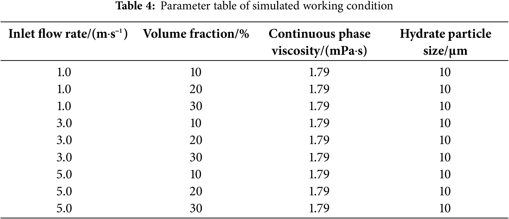
The simulation utilized values for hydrate volume fraction, flow rate, and other conditions sourced from the literature. The aim was to simulate and analyze how these factors, specifically hydrate volume fraction and flow rate within the pipe, impact hydrate particle aggregation, and to investigate the flow behavior of hydrate particles across various conditions, as presented in Table 4.

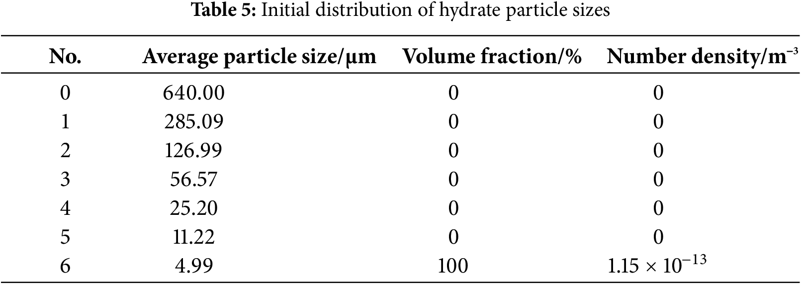
Under all simulation conditions, the hydrate particles were given the same initial particle size of approximately 5 microns to ensure comparability of the experimental data. The initial size distribution of these particles was established using the population equilibrium model, and Table 5 provides a summary of these initial particle size distributions.

5.1 Concentration Distribution of Hydrate in the Riser

The simulated results for concentration distribution in the outlet section, across various working conditions, revealed through the cloud map that all conditions exhibited consistent suspension flows. Additionally, Figs. 4 and 5 depict the hydrate concentration distribution at the outlet section of the development riser, considering different inlet flow rates and volume fractions.

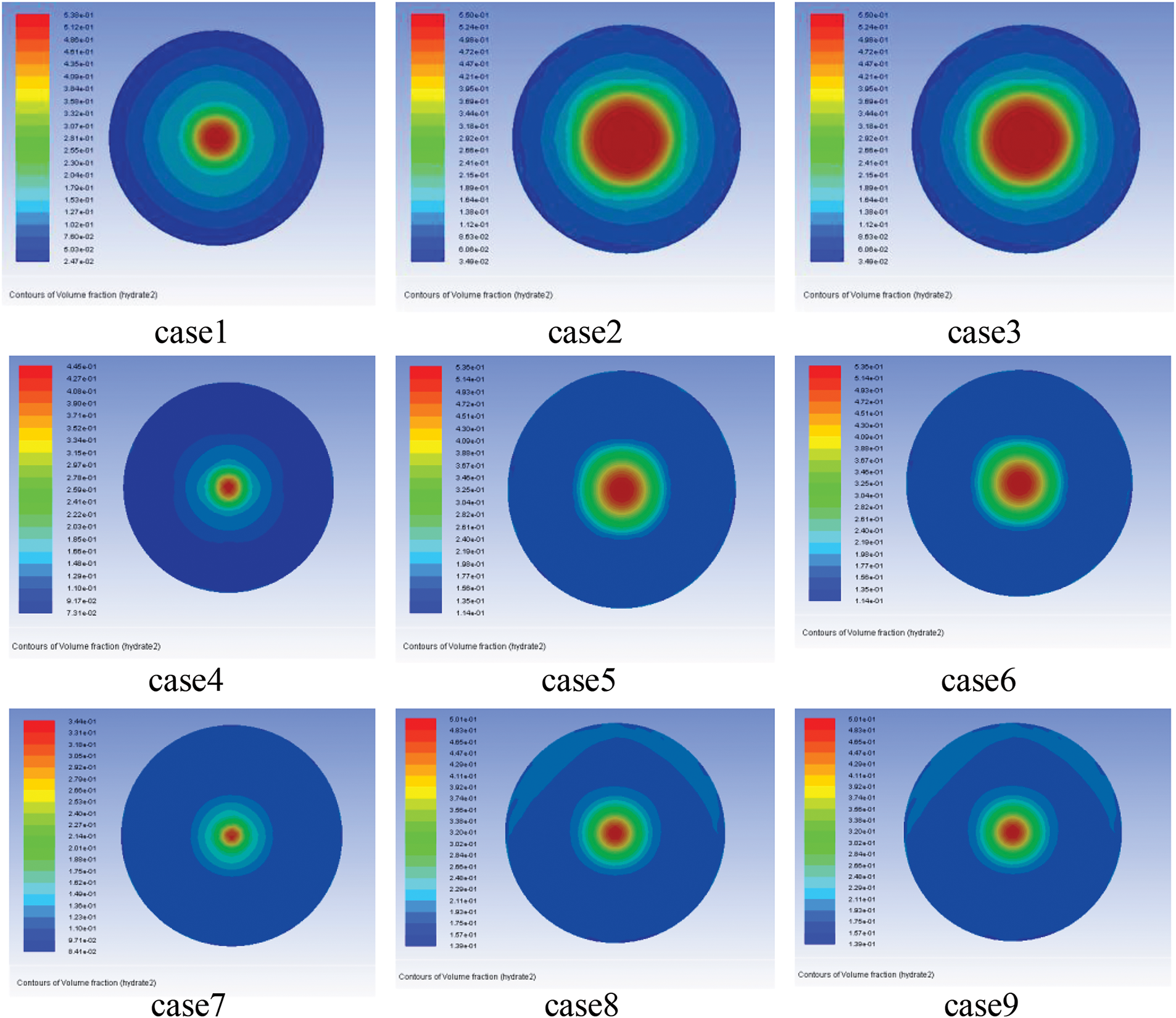
Figure 4: Cloud chart of concentration distribution at outlet section under different working conditions

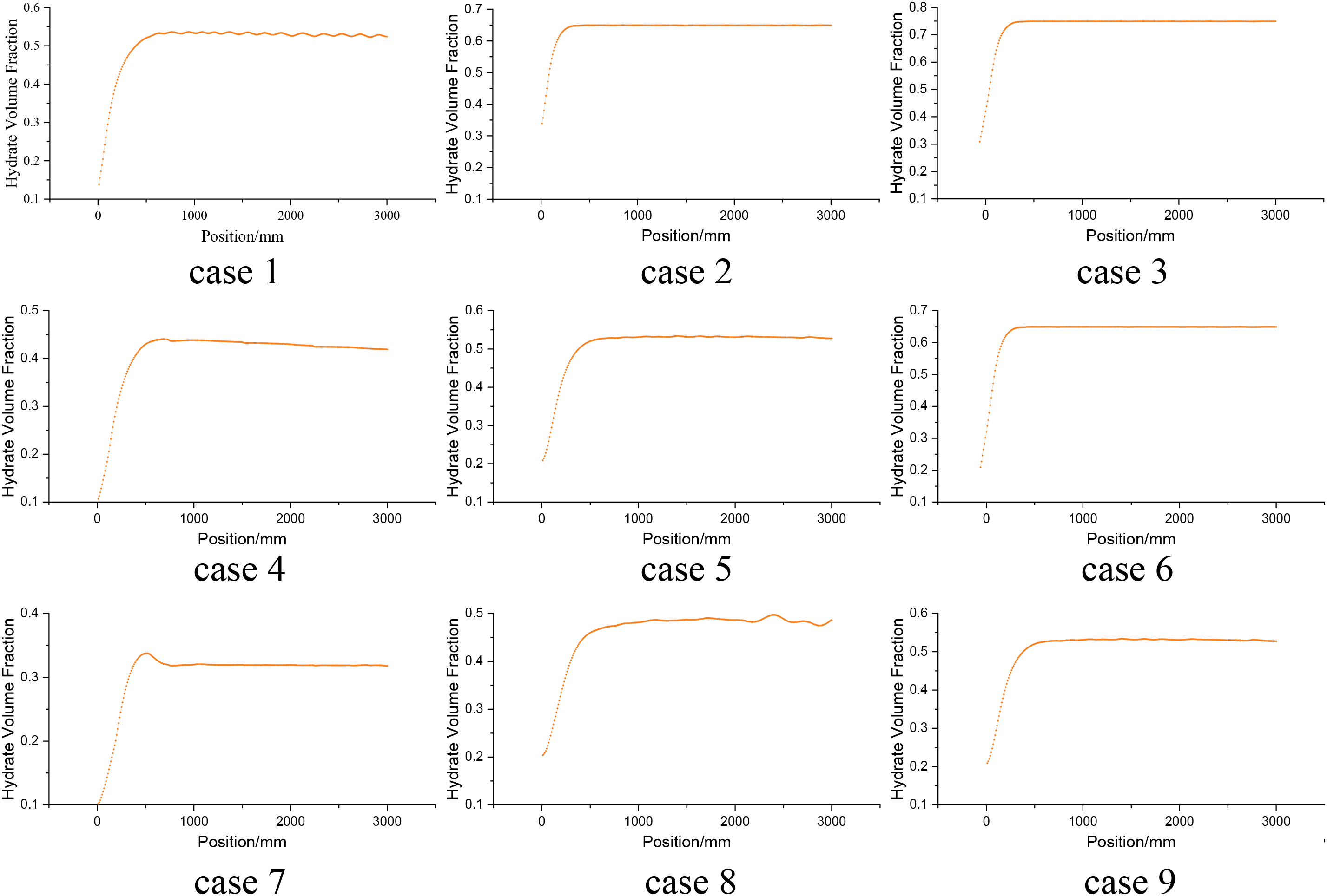
Figure 5: Axial concentration distribution of pipeline under different working conditions

Since the hydrate flow in the development riser opposes gravity, both can be envisioned as aligned in straight lines. However, due to gravity’s influence, the concentration distribution across the entire section exhibits asymmetry rather than symmetry. Furthermore, for all nine working conditions, the hydrate concentration was observed to be lower near the wall and higher in the middle. This occurs because the hydrate flow rate decreases towards the pipe wall and increases towards the center of the pipe section. As the velocity increases, the likelihood of hydrate particles colliding and aggregating also increases, resulting in a higher concentration and a more uniform distribution of these particles at the center of the pipeline section.

When the flow rate remained constant, an increase in the hydrate volume fraction led to a higher concentration of hydrate particles at the center of the pipeline and a corresponding decrease in concentration near the wall. Additionally, the area of high concentration in the pipeline’s middle section expanded. Conversely, as the flow rate rose, the distribution area of high hydrate concentration decreased, given the same concentration level.

The axial concentration distribution within the pipeline reflects the variation in hydrate concentration along its axis, as influenced by different inlet velocities and hydrate volume fractions. Under all working conditions, the hydrate concentration first increases and then tends toward equilibrium along the entire pipeline axis. The hydrate concentration was low in the early stages and high in the mid-to late stages.

When comparing the hydrate concentration distribution under identical inlet velocities but varying hydrate volume fractions, it was observed that an increase in hydrate volume fraction led to a corresponding increase in the stable hydrate concentration within the development riser. Conversely, when examining the concentration distribution at a constant hydrate volume fraction but different inlet flow rates, it was found that a higher hydrate flow rate resulted in a lower stable hydrate concentration.

5.2 Pressure Distribution of Hydrate Drop in the Riser

The pressure drop during hydrate flow is a critical issue in the process of riser development. Consequently, we conducted a study on the unit pressure drop of the developed riser under nine different operating conditions. The results of these hydrate-flow pressure drops are summarized in Table 6.

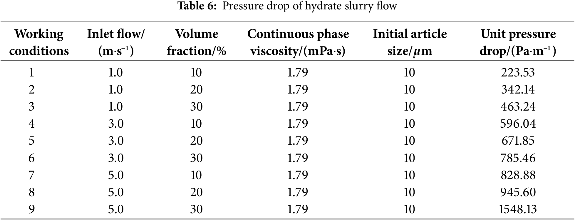
When the hydrate flow rate remained constant, the unit pressure drop increased with an increase in hydrate concentration, as indicated by the pressure drop of the hydrate flow. Simultaneously, the gradient of the unit pressure drop increased with hydrate concentration. When the hydrate volume fraction increased from 10% to 20% (double) and 30% (triple), the unit pressure drop increased by 12.72% and 31.78%, respectively. When the hydrate volume fraction was the same, the unit pressure drop increased with the hydrate flow rate. Simultaneously, the increasing gradient of the unit pressure drop increased with hydrate velocity. Taking hydrate with 10% volume fraction as an example, the unit pressure drop respectively increases 166.65% and 270.81% when the average inlet velocity increases from 1.0 to 3.0 m/s (a two-fold increase) and 5.0 m/s (a four-fold increase).

Considering working condition 1 as an example, the pressure distribution of the hydrate at different positions is shown in Fig. 6.

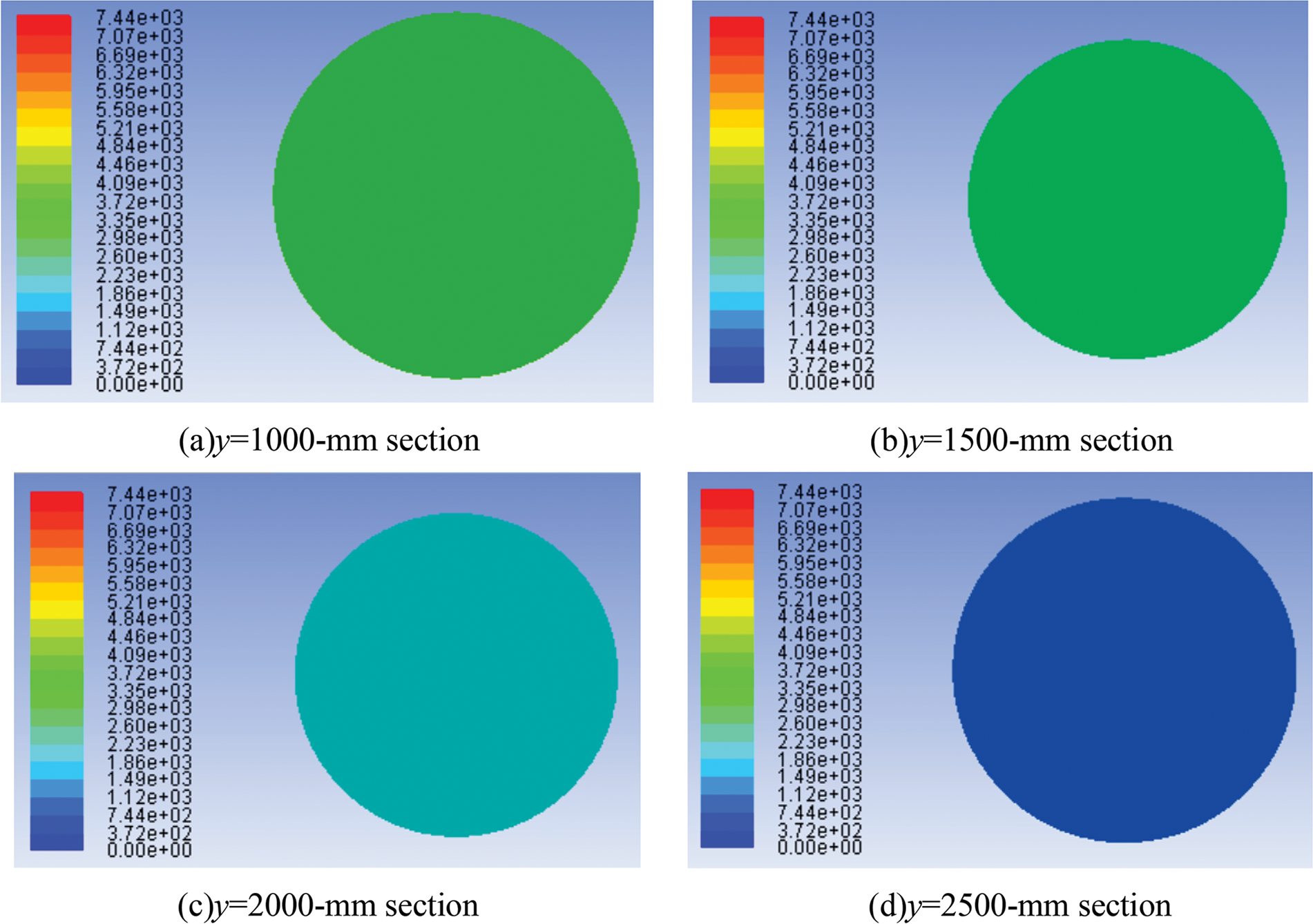
Figure 6: Pressure distribution of the main hydrate in the riser (Unit: kPa)

The trend of working condition 1 in Fig. 6 illustrates the distribution of the flow pressure drop. As the flow height changes, the pressure within the pipe decreases from 3 MPa at the bottom to 0.2 MPa. Analyzing the hydrate flow pressure drop data reveals that the primary cause of the increased unit pressure drop is the elevated flow velocity resulting from heightened hydrate flow friction in the development riser. Consequently, a higher flow velocity has an impact on the efficiency of hydrate transportation.

5.3 Velocity Distribution of Hydrate in the Riser

Based on the fully developed velocity distribution of hydrates with different volume concentrations under the same pipe diameter and different working conditions, the velocity distribution curves of the hydrate particle outlet under different pipe diameters and flow rates were drawn.

According to the characteristics of the low gas-phase content when the liquid phase was dominant, as shown in Fig. 7, the fully developed velocity distribution was consistent. The velocity at the center of the pipe section was high, the velocity near the wall was low, and the velocity developed more fully with a larger pipe diameter.

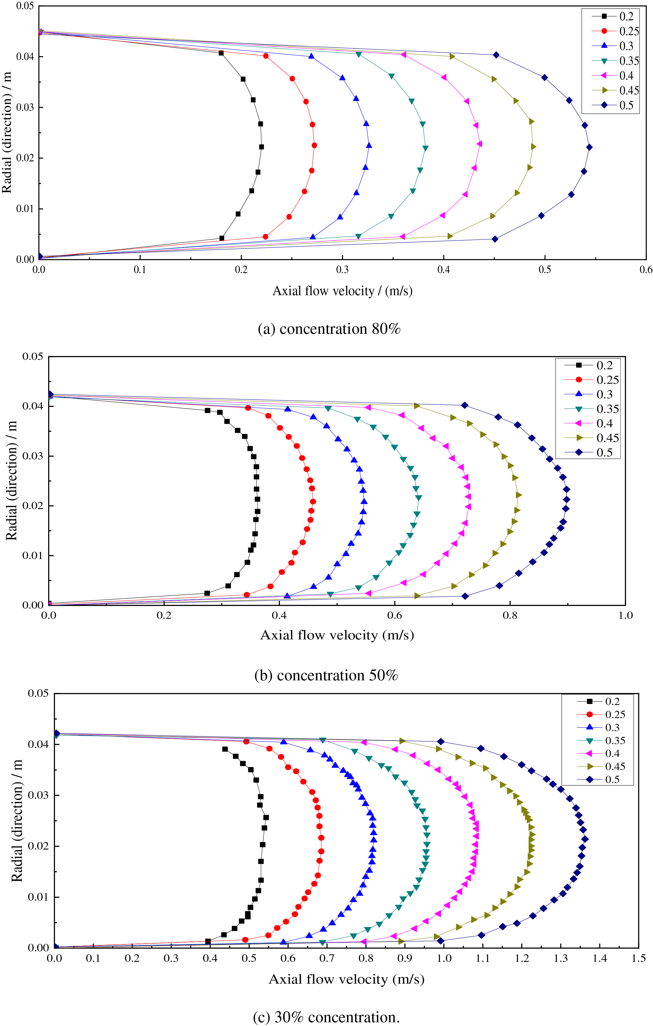
Figure 7: Outlet velocity distribution of hydrate with different concentrations under different conditions

Based on the observed trends in velocity, the behavior of the velocity curve in reaching full development was fundamentally consistent. A slight variation in the fully developed velocity profile was noted, where the central velocity of the curve in the pipe was higher at larger liquid content and high velocities compared to smaller liquid content. Under these conditions, velocity development was more pronounced, and the velocity phase was uniformly distributed about the axis of symmetry. For the same concentration, the hydrate concentration near the axis of symmetry remained stable.

6  Heat Transfer Law of Hydrate Flow in the Riser

6.1 Effect of Hydrate Flow Rate on Hydrate Heat Transfer

The effect of hydrate flow on hydrate heat transfer was studied by simulating the ambient ocean temperature in the South China Sea. The temperature environment of 10°C is set during the production process and the initial temperature of hydrate is set to 3°C. The gathering and transportation flow rates in the riser were 0.5, 1.0, and 1.5 m/s. Under the condition of a certain heat exchange coefficient, the temperature drop curves of natural gas hydrates with different flow rates were obtained, as shown in Fig. 8.

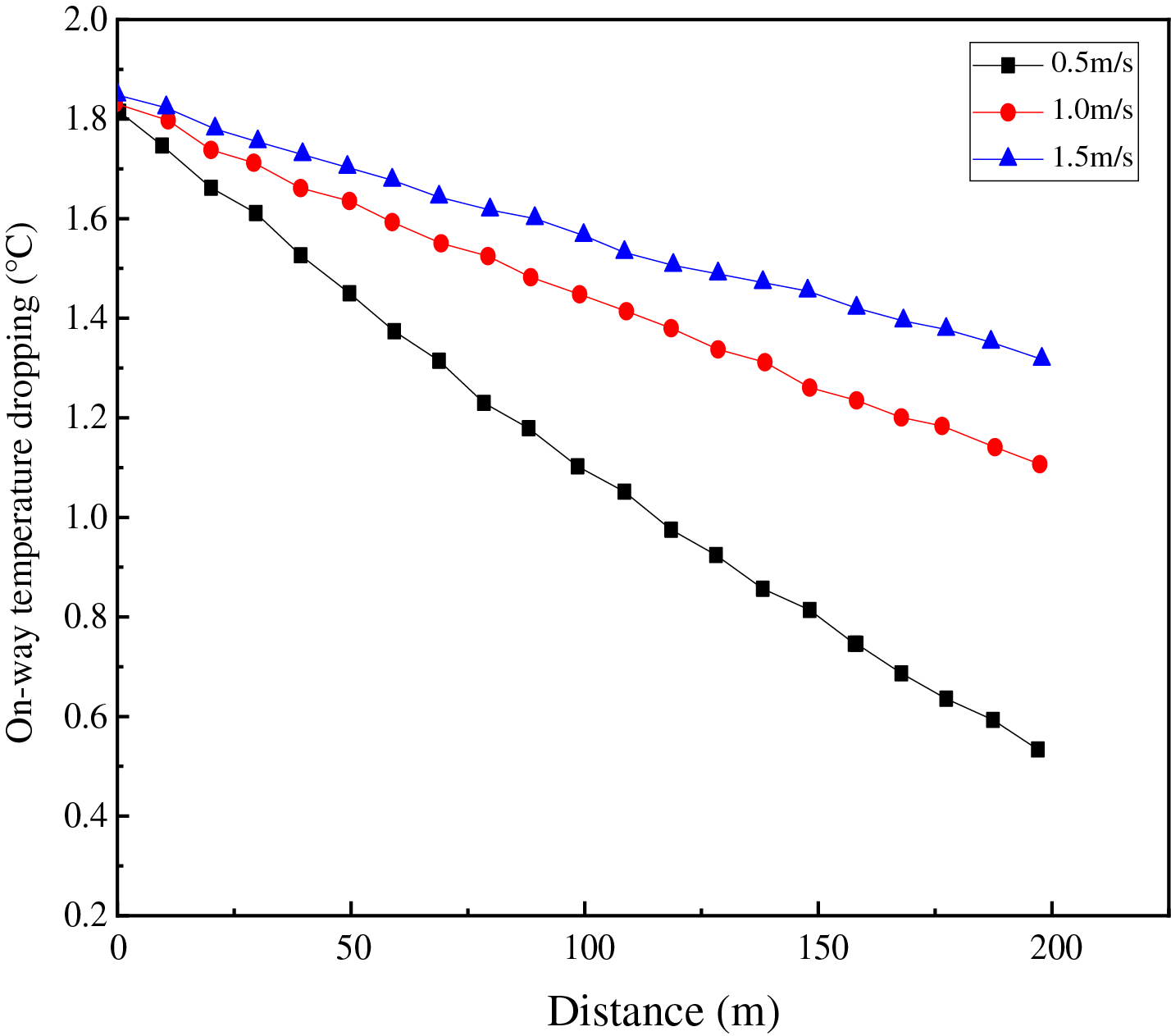
Figure 8: Temperature drop curve of natural gas hydrate with different flow rates

When all other conditions remained constant, the temperature drop of the hydrate increased as the flow rate rose. This was due to the fact that, as the hydrate flow rate increased, the convective heat transfer coefficient between the hydrate and the pipe’s inner wall decreased, leading to a weakening of the heat transfer between them. Consequently, the hydrate experienced a greater temperature drop with increasing flow rate. While enhancing heat transfer in the hydrate development riser could potentially increase the hydrate flow rate, it should be noted that as the flow rate increases, so does the friction resistance and pressure energy loss. Therefore, a balanced consideration of the hydrate transport velocity is necessary.

6.2 Effect of Seawater Temperature on Hydrate Heat Transfer

The influence of seawater temperature on the heat transfer of hydrate was studied, and the ambient temperature of the South China Sea was simulated from 4°C on the deep water bottom to 20°C on the sea level. The temperature values were 5°C, 10°C, 15°C and 20°C for comparison. The initial temperature of the hydrate was set at 3°C, and the collecting and transporting flow rate in the riser was 1.0 m/s. When the heat transfer coefficient was constant, the temperature drop curves of the NGH at different seawater temperatures were obtained, as shown in Fig. 9.

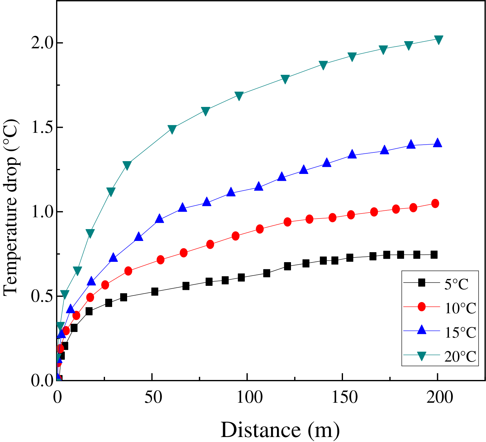
Figure 9: Temperature drop curve of natural gas hydrate with different sea water temperature

As illustrated in Fig. 9, the seawater temperature had a notable impact on the temperature drop of the hydrate within the pipeline, given the same heat transfer power. Specifically, within the temperature range of 5°C to 15°C, the heat transfer efficiency was relatively lower compared to the range of 15°C to 20°C. This discrepancy arose due to an enhancement in the convective heat transfer coefficient, which resulted in a greater temperature differential between the hydrate and the pipeline’s inner wall. Consequently, the intensity of heat exchange between the hydrate and the pipeline increased. Additionally, frictional heating elevated the temperatures of both the hydrate and the surrounding water, resulting in more significant temperature fluctuations. Consequently, when the temperature difference between the hydrate and the surrounding environment was smaller, the hydrate remained in a relatively stable state. Additionally, the hydrate is typically located several hundred meters below the seabed, where it exists in a long-term low-temperature environment. During extraction, the higher ocean temperature creates a significant temperature difference between the hydrate and its surroundings. This large temperature gradient enhances heat transfer efficiency, resulting in a higher rate of temperature drop.

The temperature distribution at the riser outlet was simulated for various seawater temperatures. Under identical conditions, the seawater temperature surrounding the pipe was varied, while all other parameters were kept constant. By altering the seawater temperature during contact, different outlet temperatures were obtained, as illustrated in Fig. 10.

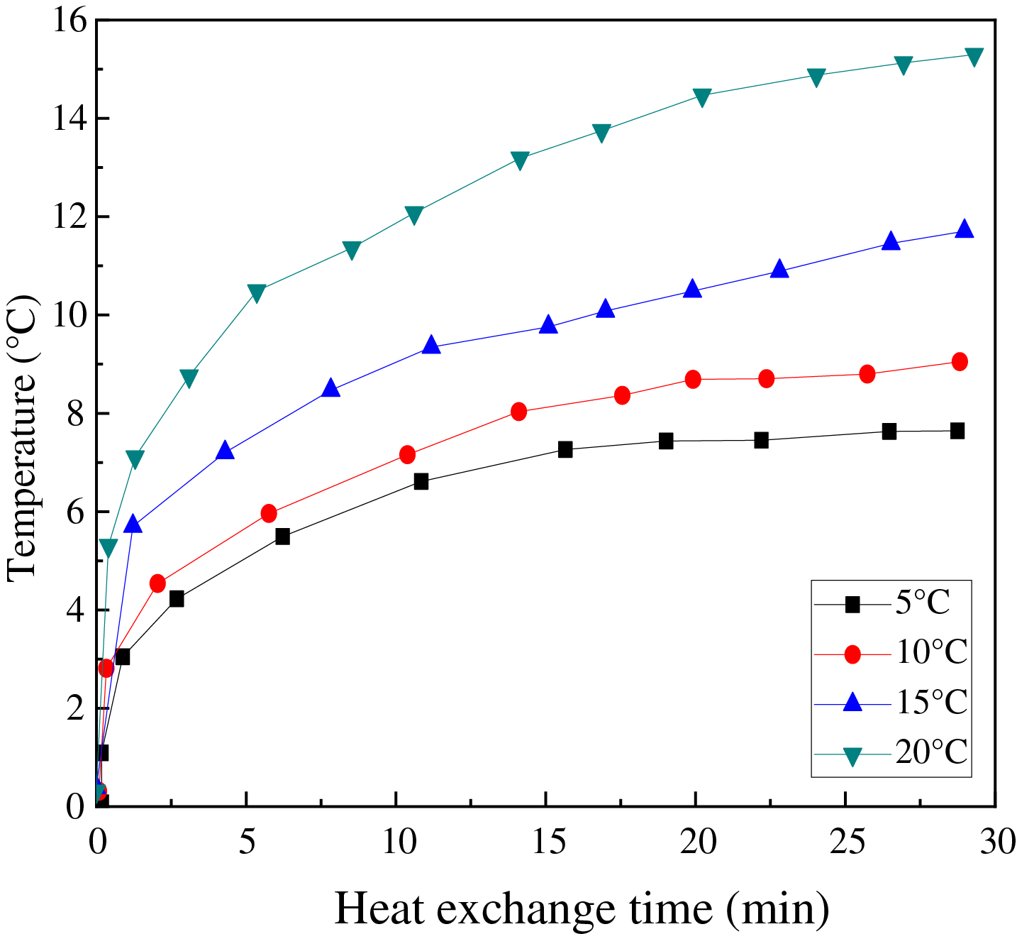
Figure 10: Riser outlet temperature with different sea water temperature

The analysis of various seawater and outlet temperatures revealed that the outlet temperature of the riser increased with a rise in the seawater temperature within the riser. This phenomenon occurs because, as the seawater temperature increases, the convective heat transfer coefficient between the hydrate and the inner wall of the riser also increases. Consequently, the heat transfer between the hydrate and the pipeline intensifies, leading to a higher outlet temperature as the seawater temperature rises.

7  Conclusion

In this study, the RNG k-ϵ turbulence model, the mass equilibrium model for hydrate particle aggregation dynamics, and the heat transfer decomposition model were employed to simulate the flow characteristics of hydrate grout in a riser. The following conclusions were drawn:

(1) Within the development riser, higher hydrate volume fractions resulted in smaller maximum particle sizes at the center of the outlet section and a larger gradient in the particle size distribution. Higher hydrate velocities were associated with smaller maximum particle sizes. Moreover, a higher hydrate volume fraction led to a higher concentration of stabilized hydrates in the developed riser. Conversely, at higher hydrate flow rates, the concentration of stabilized hydrates decreased.

(2) The primary factor contributing to the increase in unit pressure drop was the elevated flow velocity caused by the rising friction of hydrate flow within the development riser. Consequently, higher flow velocities adversely affected the efficiency of hydrate transportation. At high liquid content, the central velocity was greater than that at low liquid content, and the velocity was more fully developed. The velocity near the axis of symmetry was evenly distributed.

(3) An analysis of the flow rate and outlet temperature demonstrated that the outlet temperature of the riser increased as the hydrate flow rate rose. Under specific heat loss conditions, the flow rate must exceed a certain threshold to ensure safe transportation. However, as the hydrate flow rate increased, the pressure energy loss and frictional resistance in the pipe also rose. Therefore, selecting an optimal flow rate is essential for practical engineering applications.

(4) From the analysis of varying seawater and outlet temperatures, it was observed that the outlet temperature of the riser increased with an increase in the seawater temperature surrounding the riser. This occurred because a rise in seawater temperature enhanced the convective heat transfer coefficient between the hydrate and the inner wall of the riser, thereby intensifying the heat transfer between the hydrate and the pipe.

The findings of this study provide valuable insights for the design of flow and heat exchange systems in deep-water and shallow-water mining of hydrate deposits. Future research could focus on further refining the multiphase flow calculation model for natural gas hydrates involving phase transitions. Additionally, addressing the unique characteristics of deep-water hydrate reservoir drilling, thermodynamic conditions such as temperature fields in the upper and lower layers of the seabed and within the wellbore riser can be investigated. Based on these studies, foundational assumptions could be formulated to develop a more accurate and comprehensive theoretical framework.

Acknowledgement: Thanks to the State Key Laboratory of Low Carbon Catalysis and Carbon Dioxide Utilization for supporting this work.

Funding Statement: This work was supported by the Ministry of Industry and Information Technology High Tech Ship Special Project (Grant No. CBG3N21-2-6).

Author Contributions: The authors confirm contribution to the paper as follows: study conception and design: Chenhong Li, Guojin Han; data collection: Hua Zhong, Chao Zhang; analysis and interpretation of results: Rui Zhang, Xuewen Cao; draft manuscript preparation: Chen Xing, Chenhong Li, Jiang Bian; revision: Jonggeun Choe, Jiang Bian. All authors reviewed the results and approved the final version of the manuscript.

Availability of Data and Materials: The datasets generated and analyzed during the current study are available from the corresponding author on reasonable request.

Ethics Approval: Not applicable.

Conflicts of Interest: The authors declare no conflicts of interest to report regarding the present study.

References

1. Md-Nahin M, Guo B. A feasibility study of using geothermal energy to enhance natural gas production from offshore gas hydrate reservoirs by CO2 swapping. Energ Eng. 2023;120(12):2707–20. doi:10.32604/ee.2023.042996. [Google Scholar] [CrossRef]

2. Guo G, Chen L, Li J, Yan S, Wu W, Li L, et al. Research on the influencing rules of gas hydrate emission dissipation coefficient based on subspace spectrum clustering. Energ Eng. 2020;117(2):79–88. doi:10.32604/EE.2020.010529. [Google Scholar] [CrossRef]

3. Li B, Zhang T, Wan Q, Feng J, Chen L, Wei W. Kinetic study of methane hydrate development involving the role of self-preservation effect in frozen sandy sediments. Appl Energ. 2021;300:117398. doi:10.1016/j.apenergy.2021.117398. [Google Scholar] [CrossRef]

4. Li B, Chen L, Wan Q, Han X, Wu Y, Luo Y. Experimental study of frozen gas hydrate decomposition towards gas recovery from permafrost hydrate deposits below freezing point. Fuel. 2020;280:118557. doi:10.1016/j.fuel.2020.118557. [Google Scholar] [CrossRef]

5. Wei W, Li B, Gan Q, Li Y. Research progress of natural gas hydrate exploitation with CO2 replacement: a review. Fuel. 2022;312:122873. doi:10.1016/j.fuel.2021.122873. [Google Scholar] [CrossRef]

6. Zhang G, Li J, Liu G, Yang H, Wang C, Huang H. A developed transient gas–liquid–solid flow model with hydrate phase transition for solid fluidization exploitation of marine natural gas hydrate reservoirs. Petrol Sci. 2023;20(3):1676–89. doi:10.1016/j.petsci.2022.11.008. [Google Scholar] [CrossRef]

7. Wei N, Qiao Y, Liu A, Zhao J, Zhang L, Xue J. Study on structure optimization and applicability of hydro cyclone in natural gas hydrate exploitation. Front Earth Sci. 2022;10:991208. doi:10.3389/feart.2022.991208. [Google Scholar] [CrossRef]

8. Chen W, Xu H, Kong W, Yang F. Study on three-phase flow characteristics of natural gas hydrate pipeline transmission. Ocean Eng. 2020;214(8):107727. doi:10.1016/j.oceaneng.2020.107727. [Google Scholar] [CrossRef]

9. Lv X, Xu K, Liu Y, Wang C, Peng M, Du H, et al. Numerical simulation analysis of stable flow of hydrate slurry in gas-liquid-solid multiphase flow. Ocean Eng. 2024;300(3–4):117336. doi:10.1016/j.oceaneng.2024.117336. [Google Scholar] [CrossRef]

10. Duan X, Shi B, Wang J, Song S, Liu H, Li X, et al. Simulation of the hydrate blockage process in a water-dominated system via the CFD-DEM method. J Nat Gas Sci Eng. 2021;96(1):104241. doi:10.1016/j.jngse.2021.104241. [Google Scholar] [CrossRef]

11. Balakin B, Hoffmann A, Kosinski P. Experimental study and computational fluid dynamics modeling of deposition of hydrate particles in a pipeline with turbulent water flow. Chem Eng Sci. 2011;66(4):755–65. doi:10.1016/j.ces.2010.11.034. [Google Scholar] [CrossRef]

12. Balakin B, Hoffmann A, Kosinski P. Population balance model for nucleation, growth, aggregation, and breakage of hydrate particles in turbulent flow. AIChE J. 2010;56(8):2052–62. doi:10.1002/aic.12122. [Google Scholar] [CrossRef]

13. Fatnes E. Numerical simulations of the flow and plugging behaviour of hydrate particles [MS thesis]. Norway: The University of Bergen; 2010. [Google Scholar]

14. Jiang G, Wang X, Sun P. Numerical simulation of hydrate slurry flow based on orthogonal design. Sci Technol Rev. 2014;32(13):23–7. doi:10.3981/j.issn.1000-7857.2014.13.003. [Google Scholar] [CrossRef]

15. Song G, Li Y, Wang W, Jiang W, Shi Z, Yao S. Investigation on the mechanical properties and mechanical stabilities of pipewall hydrate deposition by modelling and numerical simulation. Chem Eng Sci. 2018;192(44):477–87. doi:10.1016/j.ces.2018.07.055. [Google Scholar] [CrossRef]

16. Song G, Li Y, Wang W, Jiang K, Shi Z, Yao S. Hydrate agglomeration modelling and pipeline hydrate slurry flow behavior simulation. Chin J Chem Eng. 2019;27(1):32–43. doi:10.1016/j.cjche.2018.04.004. [Google Scholar] [CrossRef]

17. Song G, Li Y, Wang W, Jiang K, Shi Z, Yao S. Numerical simulation of hydrate slurry flow behavior in oil-water systems based on hydrate agglomeration modelling. J Petrol Sci Eng. 2018;169(11):393–404. doi:10.1016/j.petrol.2018.05.073. [Google Scholar] [CrossRef]

18. Song G, Li Y, Wang W, Jiang K, Shi Z, Yao S. Numerical simulation of pipeline hydrate particle agglomeration based on population balance theory. J Nat Gas Sci Eng. 2018;51(11):251–61. doi:10.1016/j.jngse.2018.01.009. [Google Scholar] [CrossRef]

19. Zhou S, Zhao J, Li Q, Chen W, Zhou J, Wei N, et al. Optimal design of the engineering parameters for the first global trial production of marine natural gas hydrates through solid fluidization. Nat Gas Ind. 2018;5(2):118–31. doi:10.1016/j.ngib.2018.01.004. [Google Scholar] [CrossRef]

20. Liu Y, Tang X, Hu K. Study on flow characteristics of natural gas hydrate slurry with decomposition in vertical tube. Chem Bull. 2018;81(3):267–73. doi:10.14159/j.cnki.0441-3776.2018.03.012. [Google Scholar] [CrossRef]

21. Liang W, Lou M. Analysis of multiphase flow characteristics in a deepwater riser. P I Civil Eng-Energy. 2021;174(1):13–23. doi:10.1680/jener.19.00060. [Google Scholar] [CrossRef]

22. Marzieh L, Fassadi CA, Bahram D, Amir HM. Computational fluid dynamics modeling of the pressure drop of an iso-thermal and turbulent upward bubbly flow through a vertical pipeline using population balance modeling approach. J Energy Resour Technol. 2022;144(10):102102. doi:10.1115/1.4053711. [Google Scholar] [CrossRef]

23. Camargo R, Palermo T. Rheological properties of hydrate suspensions in an asphaltenic crude oil. In: Proceedings of the 6th International Conference on Gas Hydrates; 2002; Vancouver, BC, Canada. Vol. 1, p. 880–5. [Google Scholar]

24. Sinquin A, Palermo T, Peysson Y. Rheological and flow properties of gas hydrate suspensions. Oil Gas Sci. 2004;59(1):41–57. doi:10.2516/ogst:2004005. [Google Scholar] [CrossRef]

25. Wang W, Liang D, Fan S. Formation and blockage of HCFC-141B hydrate in pipeline. In: Proceedings of the 6th International Conference on Gas Hydrates; 2008; Vancouver, BC, Canada. [Google Scholar]

26. Austvik T, Li X, Gjertsen LH. Hydrate plug properties: formation and removal of plugs. Ann NY Acad Sci. 2000;912(1):294–303. doi:10.1111/j.1749-6632.2000.tb06783.x. [Google Scholar] [CrossRef]

27. Langer S, Swanson RC. Implementation, realization and an effective solver of two-equation turbulence models. J Sci Comput. 2024;98(8):1–33. doi:10.1007/s10915-023-02394-0. [Google Scholar] [CrossRef]

28. Song W, Xiao R, Huang C. Experimental investigation on TBAB clathrate hydrate slurry flows in a horizontal tube: forced convective heat transfer behaviors. Int J Refrig. 2009;32(7):1801–7. doi:10.1016/j.ijrefrig.2009.04.008. [Google Scholar] [CrossRef]

29. Cao X, Yang K, Wang H, Bian J. Modelling of hydrate dissociation in multiphase flow considering particle behaviors, mass and heat transfer. Fuel. 2021;306(6964):121655. doi:10.1016/j.fuel.2021.121655. [Google Scholar] [CrossRef]

30. Gao Y, Ning Y, Xu M, Wu C, Mujumdar A, Sasmito A. Numerical investigation of aqueous graphene nanofluid ice slurry passing through a horizontal circular pipe: heat transfer and fluid flow characteristics. Int Commun Heat Mass. 2022;134(8):106022. doi:10.1016/j.icheatmasstransfer.2022.106022. [Google Scholar] [CrossRef]

31. Cai X, Chen J, Liu M, Ji Y, An S. Numerical studies on dynamic characteristics of oil-water separation in loop flotation column using a population balance model. Sep Purif. 2017;176(3):134–44. doi:10.1016/j.seppur.2016.12.002. [Google Scholar] [CrossRef]

32. Habiyaremye V, Kuerten J, Frederix E. Comparison of population balance models for polydisperse bubbly flow. Chem Eng Sci. 2023;278(17):118932. doi:10.1016/j.ces.2023.118932. [Google Scholar] [CrossRef]

33. Cao X, Yang K, Li T, Xiong N, Yang W, Bian J. Numerical simulation of hydrate particle behaviors in gas-liquid flow for horizontal and inclined pipeline. Case Stud Therm Eng. 2021;27(14):101294. doi:10.1016/j.csite.2021.101294. [Google Scholar] [CrossRef]

34. Yang X, Shyy W, Xu K. Unified gas-kinetic wave-particle method for gas-particle two-phase flow from dilute to dense solid particle limit. Phys Fluids. 2022;34(2):023312. doi:10.1063/5.0081105. [Google Scholar] [CrossRef]

35. Abrahamson J. Collision rates of small particles in a vigorously turbulent fluid. Chem Eng Sci. 1975;30(11):1371–9. doi:10.1016/0009-2509(75)85067-6. [Google Scholar] [CrossRef]

36. Cao X, Yang K, Wang H, Bian J. Gas–liquid–hydrate flow characteristics in vertical pipe considering bubble and particle coalescence and breakage. Chem Eng Sci. 2022;252(6964):117249. doi:10.1016/j.ces.2021.117249. [Google Scholar] [CrossRef]

37. Stamatiou E. Experimental study of the ice slurry thermal-hydraulic characteristics in compact plate heat exchangers. Ottawa, ON, Canada: National Library of Canada; 2004. [Google Scholar]

38. Galkin V, Zharov V. Exact solutions of the Boltzmann-Maxwell kinetic equation. J Appl Math Mech. 2004;68(1):1–23. doi:10.1016/S0021-8928(04)90001-9. [Google Scholar] [CrossRef]

39. Li L, Loyalka S, Tamadate T, Sapkota D, Ouyang H, Hogan C. Measurements of the thermophoretic force on submicrometer particles in gas mixtures. J Aerosol Sci. 2024;178:106337. doi:10.1016/j.jaerosci.2024.106337. [Google Scholar] [CrossRef]

40. Patra P, Roy A. Brownian coagulation of like-charged aerosol particles. Phys Rev Fluids. 2022;7(6):064308. doi:10.1103/PhysRevFluids.7.064308. [Google Scholar] [CrossRef]

41. Chen M, Cheng L, Wang X, Lyu C, Cao R. Pore network modelling of fluid flow in tight formations considering boundary layer effect and media deformation. J Petrol Sci Eng. 2019;180(7):643–59. doi:10.1016/j.petrol.2019.05.072. [Google Scholar] [CrossRef]