
 Submit a Paper
 Propose a Special lssue
 Open Access
ARTICLE

Impact of Dataset Size on Machine Learning Regression Accuracy in Solar Power Prediction
1 Department of Electrical and Electronic Engineering, International University of Business Agriculture and Technology, Dhaka, 1230, Bangladesh
2 Department of Electrical and Electronic Engineering, Dhaka University of Engineering and Technology, Gazipur, 1707, Bangladesh
3 Department of Electrical Engineering, INTI International University, Persiaran Perdana BBN, Putra Nilai, Nilai, 71800, Malaysia
4 Department of Mechanical Engineering, International University of Business Agriculture and Technology, Dhaka, 1230, Bangladesh
5 Department of Sustainable and Renewable Energy Engineering, University of Sharjah, Sharjah, 27272, United Arab Emirates
* Corresponding Author: Mamdouh Assad. Email:
(This article belongs to the Special Issue: Advances in Renewable Energy Systems: Integrating Machine Learning for Enhanced Efficiency and Optimization)
Energy Engineering 2025, 122(8), 3041-3054. https://doi.org/10.32604/ee.2025.066867
Received 19 April 2025; Accepted 19 June 2025; Issue published 24 July 2025
 View Full Text
 Download PDF
Abstract
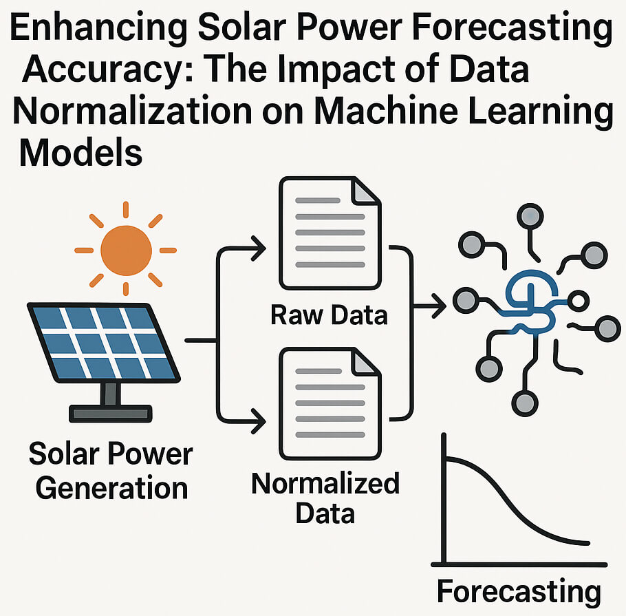
Knowing the influence of the size of datasets for regression models can help in improving the accuracy of a solar power forecast and make the most out of renewable energy systems. This research explores the influence of dataset size on the accuracy and reliability of regression models for solar power prediction, contributing to better forecasting methods. The study analyzes data from two solar panels, aSiMicro03036 and aSiTandem72-46, over 7, 14, 17, 21, 28, and 38 days, with each dataset comprising five independent and one dependent parameter, and split 80–20 for training and testing. Results indicate that Random Forest consistently outperforms other models, achieving the highest correlation coefficient of 0.9822 and the lowest Mean Absolute Error (MAE) of 2.0544 on the aSiTandem72-46 panel with 21 days of data. For the aSiMicro03036 panel, the best MAE of 4.2978 was reached using the k-Nearest Neighbor (k-NN) algorithm, which was set up as instance-based k-Nearest neighbors (IBk) in Weka after being trained on 17 days of data. Regression performance for most models (excluding IBk) stabilizes at 14 days or more. Compared to the 7-day dataset, increasing to 21 days reduced the MAE by around 20% and improved correlation coefficients by around 2.1%, highlighting the value of moderate dataset expansion. These findings suggest that datasets spanning 17 to 21 days, with 80% used for training, can significantly enhance the predictive accuracy of solar power generation models.Graphic Abstract
Keywords
Producing solar power is crucial for meeting the world’s energy needs and reducing the environmental effects of traditional energy sources. With advancements in solar technology and growing ecological consciousness, solar power is increasingly becoming a pivotal component of the renewable energy landscape [1]. However, to effectively harness solar energy, accurate prediction of solar power generation is essential, as it depends on variables like location, weather, and time of day.
Applying machine learning (ML) techniques has significantly improved solar power forecasting by enabling models to learn from historical patterns and predict future outputs more accurately [2]. Recent research has demonstrated the superior capability of deep learning and ensemble-based methods, such as LSTM, CNN, Random Forest, and Gradient Boosting, in capturing non-linear dependencies and improving predictive performance compared to traditional statistical methods. For instance, Ref. [3] used a hybrid LSTM-XGBoost model for solar irradiance prediction and reported substantial accuracy gains under dynamic weather conditions. Similarly, Ref. [4] showed that ensemble models like Random Forest and AdaBoost outperformed standalone algorithms regarding reliability and stability in solar forecasting tasks.
Regression, in particular, remains widely adopted for solar power prediction tasks due to its suitability for modeling continuous output variables such as energy generation levels. Recent advances also highlight integrating feature selection and data preprocessing techniques to boost regression model performance. For example, Ref. [5] demonstrated that applying Min-Max normalization significantly reduced RMSE in SVR and ANN-based solar prediction models, while Ref. [6] highlighted how normalization improves convergence in neural networks.
The performance of ML algorithms in predicting solar power generation is highly dependent on the quality and quantity of the data used for training. Dataset size is essential in determining a model’s accuracy and generalization capability. Larger datasets yield better performance by reducing overfitting, although they come with increased preprocessing and computational demands [7]. However, Ref. [8] argued that increasing data size shows diminishing returns beyond a certain threshold unless accompanied by relevant feature selection and data refinement strategies.
There isn’t a single accepted definition of what constitutes an optimal dataset; instead, different researchers [9] have explored diverse heuristics and empirical methods to define ideal dataset compositions regarding volume, diversity, and quality.
This study investigates the impact of dataset size on the regression performance of ML algorithms for predicting solar power generation. By systematically varying training dataset sizes and evaluating model performance, the study aims to understand how data volume affects accuracy and robustness in solar prediction tasks.
The key contributions of this study include: (i) a comparative analysis of normalized vs. raw data input on various machine learning models for solar energy prediction; (ii) evaluation of model robustness across different data split percentages; and (iii) evidence of improved prediction accuracy with normalization, especially for neural network-based models. These contributions extend prior works by providing a detailed quantification of normalization impacts.
This study offers a novel contribution by systematically investigating how the size of short-term datasets affects the predictive performance of regression models in solar power generation. This topic has received limited attention in prior research. While earlier research mainly looked at comparing models or predicting over long periods, our study examines explicitly how different dataset lengths (7–38 days) affect six standard regression models using actual solar panel data. Unlike most literature that emphasizes either model optimization or feature selection, this study offers numerical details about the minimum effective dataset length required to achieve reliable predictions, focusing on MAE reduction and correlation improvements. Furthermore, using two different panel types enhances the generalizability of the findings. This research provides practical guidelines for solar energy analysts and researchers regarding the trade-off between data volume and model accuracy, particularly when data availability is limited.
The National Renewable Energy Laboratory (NREL) is a national laboratory of the United States Department of Energy that provided the data utilized in this study. Every day, NREL uses the Internet to retrieve the data stored in a database. Data that did not meet quality requirements were excluded using quality assurance (QA) techniques [10].
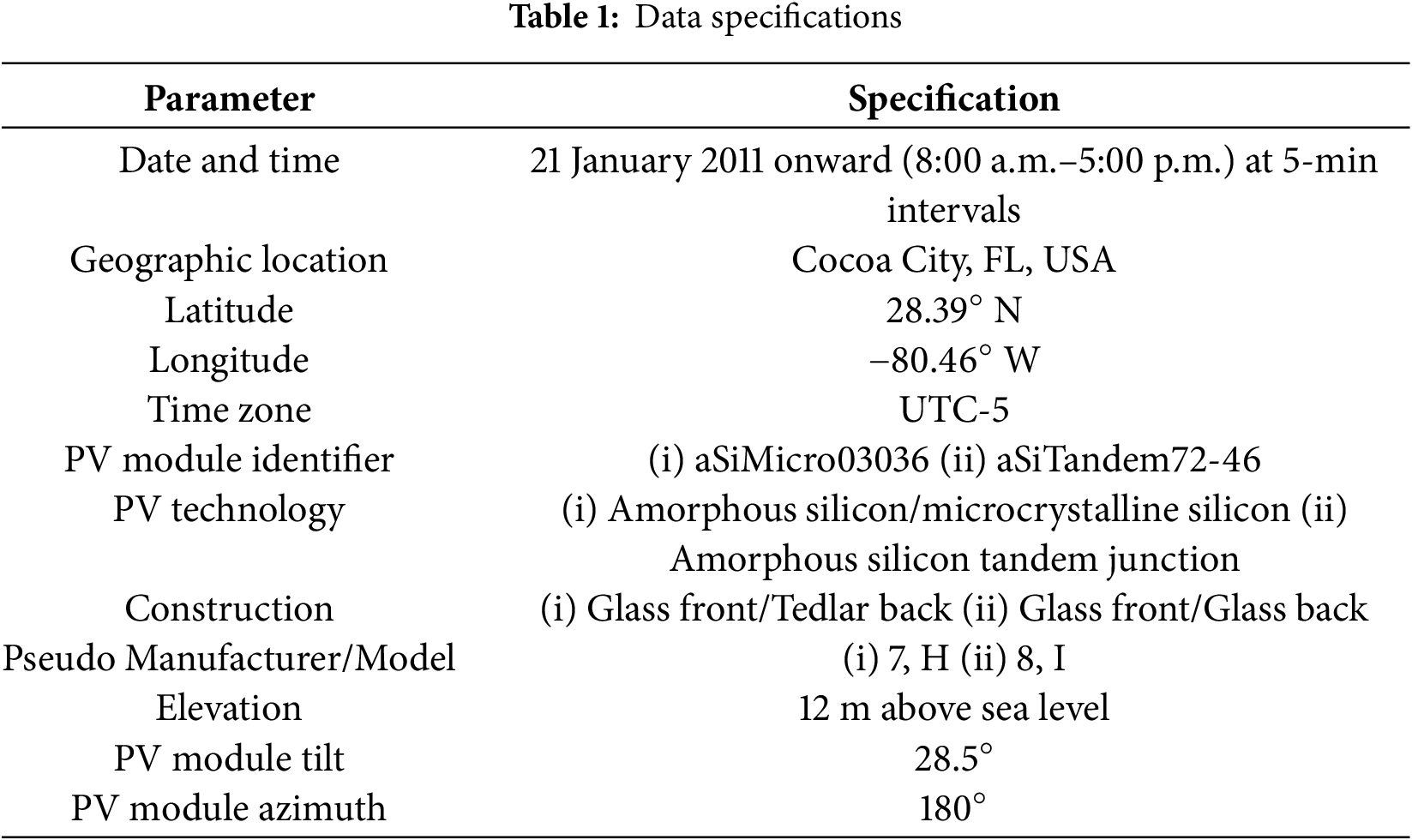
This study used data from 40 days to ensure high-quality, consistent data with minimal missing values and noise. The limited timeframe allowed for a controlled evaluation of the effects of data normalization on model performance without introducing seasonal variability. It also enabled faster experimentation, aligning with the study’s focus on methodology rather than long-term forecasting. Table 1 presents an overview of the data specifications.
The study evaluates five machine learning algorithms for solar power prediction: a simple method of linear Regression that captures linear relationships (as a baseline model); support vector machine learning for regression tasks (SMOreg), which can model non-linear relationships using kernel tricks; Multilayer Perceptron (MLP/ANN), a type of neural network that accommodates complex non-linearities; random forest, an ensemble of decision trees that are robust to noise; and k-Nearest Neighbors (k-NN/IBk), an instance-based learner who employs local averaging. Due to their diverse regression methods, we included these models with random forest and k-NN showing the most promise in preliminary studies. The study compares their performance across dataset sizes, using Weka’s implementation for fairness.
This investigation employed the dependable and popular open-source machine-learning program Weka, created at the University of Waikato. Weka covers a wide range of machine learning algorithms, has an intuitive interface, and is particularly well-accepted for research and teaching. Its credibility is enhanced by its thriving open-source community, frequent updates, and favorable user feedback [11].
In the data collection and preprocessing phase, datasets are gathered from two solar panels and then subjected to preprocessing steps to ensure data quality. This involves handling missing values, normalizing features, and performing other necessary data-cleaning tasks.
To ensure the accuracy and reliability of the predictive models, several data preprocessing steps were applied to address potential quality issues such as missing values, outliers, and extreme values. First, we looked at the raw dataset to find any missing entries; we filled these gaps using linear interpolation based on nearby time-series data to keep the data smooth without creating false trends. The study employed the interquartile range (IQR) method to identify outliers, identifying points more than 1.5 times the IQR away from the first or third quartile. Detected outliers were carefully reviewed, and if they were found to be due to sensor anomalies or data logging errors, they were either corrected (when ground truth was available) or removed from the dataset. Additionally, all input features were normalized using Min-Max scaling to ensure uniformity and enhance model convergence during training. These preprocessing steps ensured a clean and consistent dataset, forming a robust foundation for accurate model development and evaluation [12].
Moving on to model selection, suitable machine learning algorithms for regression tasks in Weka are chosen. These include Linear Regression (Eq. (1)), Support Vector Machine for Regression (SMOreg) (Eq. (2)), Multilayer Perceptron (MLP) (Eq. (3)), Random Forest (Eq. (4)), and k-Nearest Neighbor (k-NN) (Eq. (5)). Following model selection, the datasets are split into 80:20 training and testing sets using Weka’s built-in functions or manually. The machine learning models, formulations, and workflows are shown below.
Equation:
where y is the solar power output, xi is the feature (e.g., irradiance, temperature), βi are the coefficients, and ϵ is the error.
Workflow:
Fit coefficients via ordinary least squares (OLS) minimization.
Predict using the linear combination of features.
3.2.2 Support Vector Machine Regression (SMOreg)
SMOreg is a Support Vector Machine (SVM) variant modified for regression tasks. It effectively captures complex relationships in high-dimensional feature spaces and is less susceptible to overfitting. However, it can be computationally intensive, especially with large datasets, and requires careful selection of hyperparameters [13].
Equation (Kernel-Based Prediction):
where K(xi, x) is the RBF kernel exp(−γ∥xi−x∥2), and αi’s are the Lagrange multipliers.
Workflow:
Transform features using the RBF kernel.
Solve the dual optimization problem via sequential minimal optimization (SMO).
3.2.3 Multilayer Perceptrons (MLPs)
Multilayer Perceptron (MLP), or Artificial Neural Network (ANN), is a versatile algorithm inspired by the structure and function of biological neurons. It consists of multiple layers of interconnected neurons that process input data and propagate information through the network to produce output predictions. MLPs can capture complex non-linear relationships in data and can learn from large and diverse datasets. Training MLPs can be computationally expensive and require careful tuning of hyperparameters to prevent overfitting [14].
Equation (Forward Propagation):
where σ is ReLU activation, and W(l) are layer weights.
Workflow:
Initialize weights and biases.
Train via backpropagation with Adam optimizer (default: learning rate = 0.3).
Random Forest is an algorithm that constructs multiple decision trees during training and combines their predictions through averaging (Regression) to improve accuracy and reduce variance. Random forests are robust enough to overfit, handle numerical and categorical data well, and provide feature-importance rankings. They may be prone to overfitting with noisy datasets and can be computationally expensive, especially with many trees [15].
Equation (Ensemble Prediction):
where T is the number of trees (default: 100), and fi(x) is the individual tree predictions.
Workflow:
Bootstrap sample training data for each tree.
Split nodes using mean squared error (MSE) reduction (default: mtry = √n).
3.2.5 k-Nearest Neighbors (k-NN)
k-Nearest Neighbor (k-NN) is a simple, instance-based learning algorithm commonly used for regression tasks. It predicts the target parameter by averaging the values of the k nearest neighbors in the feature space. k-NN is easy to understand and implement and can handle complex relationships in the data without making strong assumptions about the underlying distribution. It can be computationally expensive during prediction, especially with large datasets, and the choice of the k parameter may impact the model’s performance [16].
Equation (Prediction):
where Nk(x) is the k nearest neighbors (default: k = 1).
Workflow:
Compute Euclidean distance between test and training points.
Average outputs of the k nearest neighbors.
Subsequently, model evaluation takes place. Weka’s training functionality trains each selected model on different dataset sizes. The trained models are then tested on the corresponding testing sets to evaluate their performance. Performance metrics such as correlation coefficients or mean absolute error are calculated using Weka’s evaluation tools to assess the effectiveness of each model.
The analysis stage involves interpreting the evaluation results to comprehend the impact of dataset size on regression performance for each machine learning algorithm. Fig. 1 illustrates the methodological flowchart. Appendix A provides a detailed list of the model hyperparameters, including their default settings as configured in the Weka software.
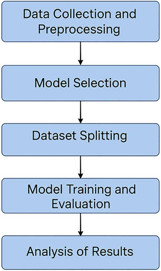
Figure 1: Flowchart outlining the steps of the methodology
The correlation coefficient and MAE are valuable evaluation metrics in comparing regression algorithms for predicting solar power generation.
The correlation coefficient indicates the direction and strength of the linear relationship between two variables. In the case of Regression, it quantifies the degree of association between the predicted values and the actual values. A correlation coefficient closer to 1 indicates a strong positive correlation, while a value closer to −1 indicates a strong negative correlation. A value near 0 suggests little to no linear relationship. A high correlation coefficient signifies that the predictions made by the regression model closely follow the actual values, indicating good predictive performance [17].
Mean Absolute Error (MAE) measures the average absolute difference between actual and predicted values. It provides a clear-cut assessment of the model’s predictive accuracy, regardless of the direction of errors. A lower MAE indicates better predictive performance, as it signifies that, on average, the model’s predictions are closer to the actual values [18]. The rationales for selecting these measures were as follows:
Correlation reflects the coherence between the directions of two solar power predictions and is essential for solar power grid integration and energy planning [19].
MAE is resistant to outliers and is directly interpretable in power production units (W/m2), which is useful for operation decisions [18]. They jointly considered both the linear relationship (correlation) and absolute size of error (MAE), producing a balanced evaluation of overall model performance.
When analyzing 80% of the training data, all machine-learning algorithms utilized in this study, except for IBk, exhibit similar responses across datasets lasting 14 days or more for both the aSiMicro03036 and aSiTandem72-46 solar panel models. Patterns demonstrated by SMOreg, Linear Regression, and ANN (MLP) remain consistent across datasets of varying sizes for both types of panels. Table 2 presents the correlation coefficients for the aSiMicro03036 panel, and a graphical representation is provided in Fig. 2.
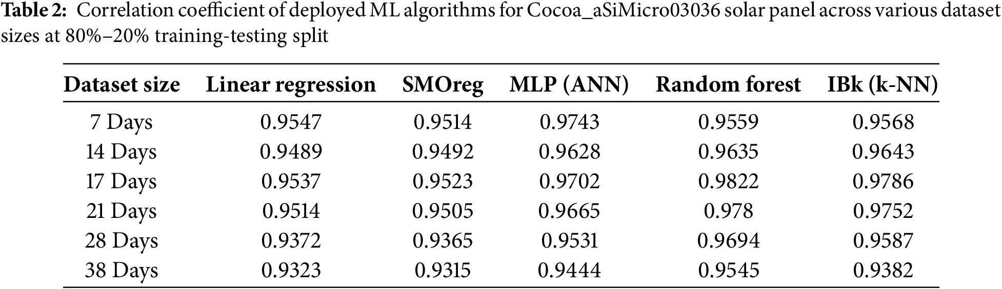
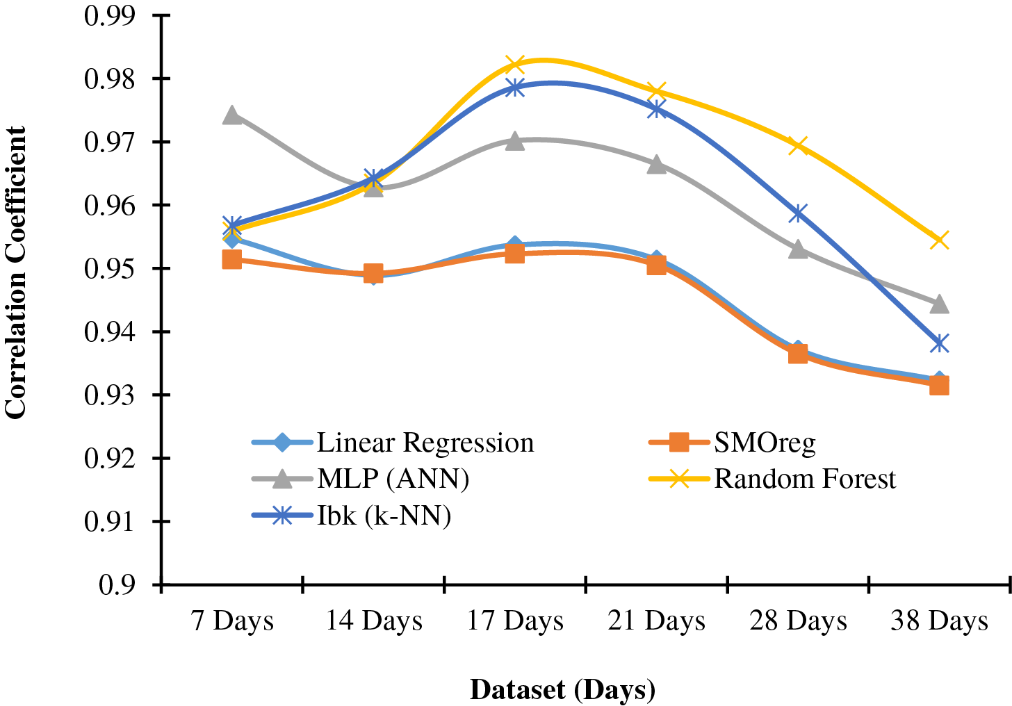
Figure 2: Graphical representation of data from Table 2
Regarding the aSiMicro03036 panel, when the dataset spans 17 days, all machine-learning models perform optimally with an 80% training set. Random Forest surpasses others with the highest correlation coefficient (0.9822). IBk shows a response akin to Random Forest, producing the second-highest correlation coefficient (0.9786) under the same conditions.
For the aSiTandem72-46 panel, with a dataset spanning 21 days, all Machine Learning models achieve peak performance with an 80% training set. Random Forest again outperforms the others with the highest correlation coefficient (0.9647). At the same time, ANN (MLP) exhibits a response similar to Random Forest, yielding the second-highest correlation coefficient (0.9531) under identical conditions. Table 3 presents the correlation coefficients for the aSiTandem72-46 panel, and a graphical representation is provided in Fig. 3.
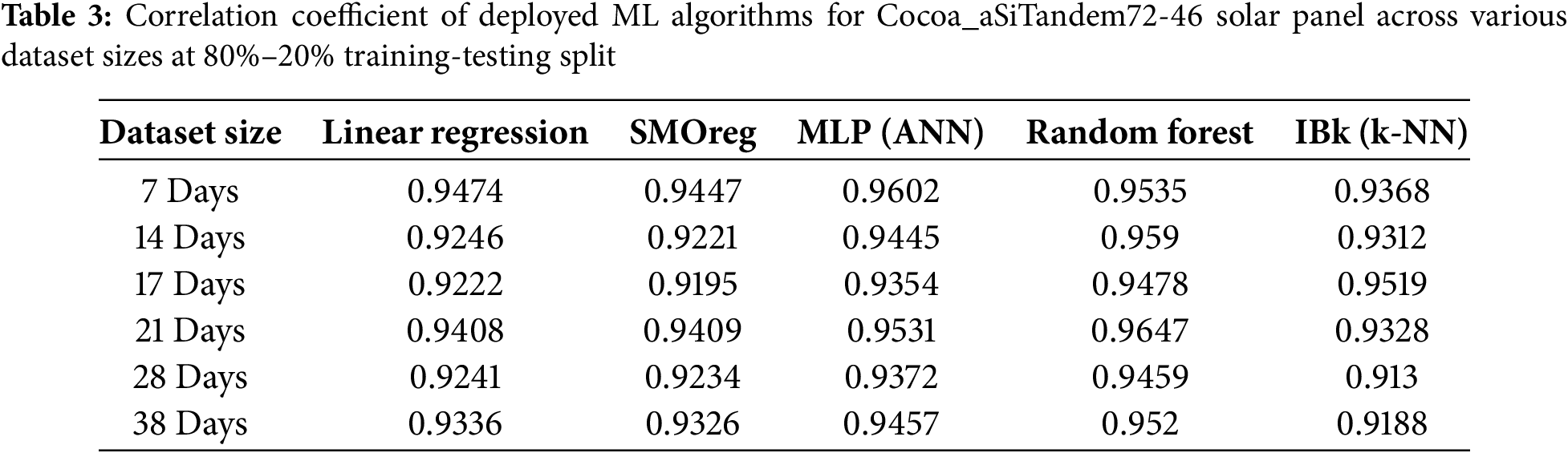
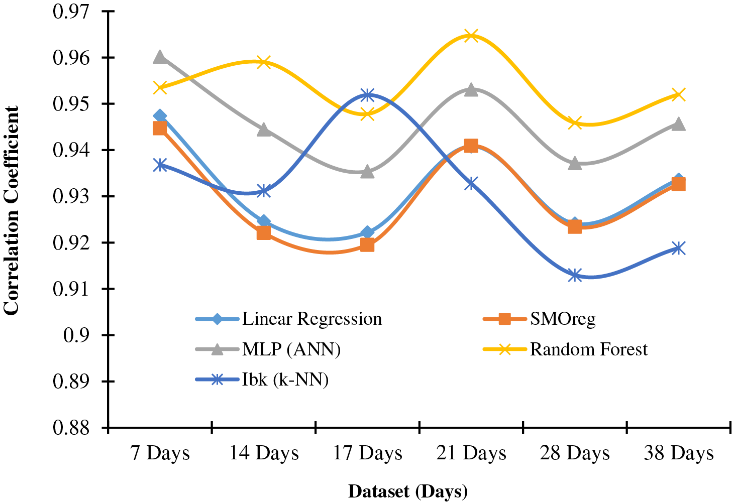
Figure 3: Graphical representation of data from Table 3
In Figs. 2 and 3, a different trend in results is observed. This can be attributed to the various characteristics of technological and manufacturing variations.
Regarding MAE, SMOreg, and Linear Regression, they exhibit similar responses for both solar panels. Random Forest and IBk demonstrate nearly identical patterns for both solar panels, comparatively better than those of SMOreg and Linear Regression. MLP (ANN) follows a similar pattern in the aSiMicro03036 panel, but it displays sharp non-linearity in the pattern for the aSiTandem72-46 panel. Table 4 presents the Mean Absolute Error for the aSiMicro03036 panel, and a graphical representation is provided in Fig. 4.
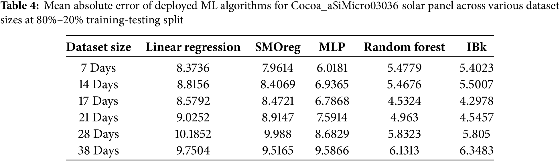
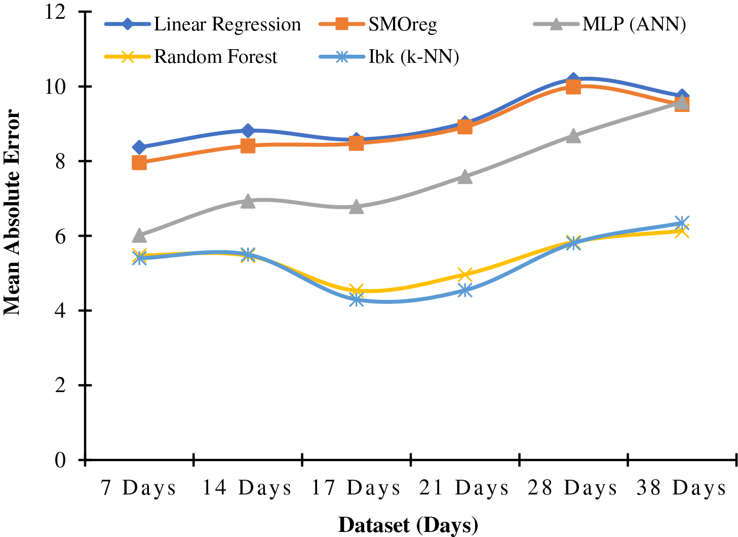
Figure 4: Graphical representation of data from Table 4
For the aSiMicro03036 panel, when the dataset spans 17 days, all Machine Learning models perform optimally with an 80% training set. IBk outperforms others with the lowest MAE of 4.2978. Random Forest shows a response similar to IBk, yielding the second-lowest MAE under the same conditions.
For the aSiTandem72-46 panel, with a dataset spanning 21 days, all Machine Learning models achieve peak performance with an 80% training set. Table 5 presents the Mean Absolute Error for the panel, and a graphical representation is provided in Fig. 5. Random Forest outperforms the others with an MAE of 2.0544. At the same time, IBk demonstrates a response similar to Random Forest, yielding the second-lowest MAE (2.1463) with a dataset spanning 17 days. In Figs. 3 and 5, IBk (k-NN) at 17 days and MLP (ANN) at 28 days show unexpected results. This can be attributed to using default parameters in those models without proper tuning.
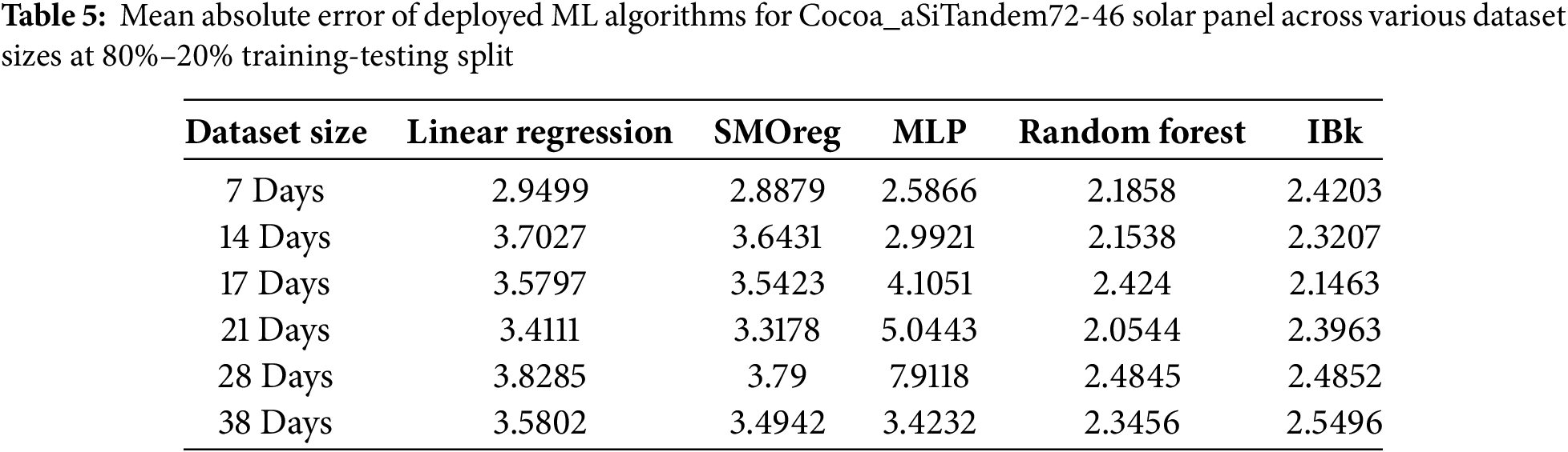
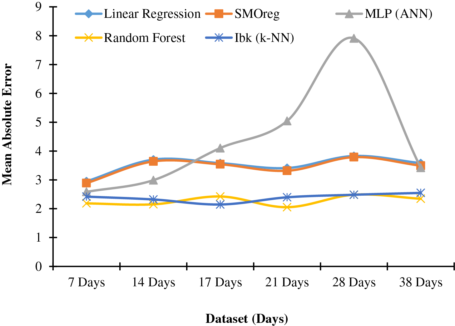
Figure 5: Graphical representation of data from Table 5
Datasets ranging from 17 to 21 days can be effectively utilized for predicting solar power generation, with 80% of the data allocated to the training set to enhance prediction accuracy.
The approach presented in this section is highly scalable due to its reliance on publicly available data and open-source tools like Weka. It is also applicable across different geographic regions by retraining the model using location-specific meteorological data.
This study explored the relationship between dataset size and the performance of machine learning algorithms in predicting solar power generation. Datasets from two solar panels over various periods were analyzed, and the performance of five algorithms—linear Regression, Support Vector Machine for Regression (SMOreg), Multilayer Perceptron (MLP), Random Forest, and k-Nearest-neighbor (IBk)—was evaluated. Across datasets lasting 14 days or more, except for IBk, algorithms showed similar responses for both aSiMicro03036 and aSiTandem72-46 panel models. Random Forest consistently outperformed others, achieving the highest correlation coefficients for both panels. Additionally, when the dataset spans 17 days, all models performed optimally for aSiMicro03036, with IBk showing the lowest MAE. Random Forest achieved the lowest MAE for aSiTandem72-46 with a dataset spanning 21 days. The study concluded that datasets ranging from 17 to 21 days, with 80% allocated to training, effectively predict solar power generation, enhancing prediction accuracy. From these insights, in the case of Regression, it can be recommended that the suitable dataset sizes for the aSiMicro03036 and aSiTandem72-46 solar panels are 17 and 21 days, respectively.
6 Implications and Future Research Opportunities
Short Period and Small Geographic Scale: The data was collected over 40 days in only one location (Cocoa City, FL, USA). This limits the results’ applicability to other seasons and regions, as solar PV power production can vary significantly with climate and season.
Univariate Normalization Only: The paper employed only min-max scaling as the data normalization method. Other normalization techniques, such as Z-score Normalization and robust scaling, were not explored and may influence the results.
Default Model Parameters: Some models (IBk and MLP) were used with default hyperparameter settings without tuning. This could explain particular unfavorable outcomes (e.g., the performance of IBk at 17 days or the excessive non-linearity of the MLP), which may not have revealed their optimal capabilities.
External Factors Not Considered: The study did not include other influential factors, such as variations in cloud cover, dust accumulation on panels, and regional differences in energy consumption patterns, which may be pertinent to the accuracy of our solar power predictions.
Short-term Data: This analysis focuses on short-term data (7 to 38 days), which may not capture long-term changes or cyclical variations in solar power generation.
6.2 Future Research Directions
Long-term Data Collection: Subsequent research should gather data over extended periods (e.g., 1–2 years) covering multiple seasons and diverse geographic locations to verify the stability of the findings across various environmental conditions.
Comparative Normalization Methods: Assess the impact of different normalization techniques (like robust scaling and Z-score) and feature selection steps on model performance to identify the most effective preprocessing strategies.
Hyperparameter Tuning: Systematically optimize parameters for all models, especially IBk and MLP, to ensure maximum performance and reduce unexpected outcomes.
External Variable Integration: To enhance the model’s accuracy and practicality, incorporate additional external variables, such as weather prediction data, panel maintenance information, and geographic factors.
Hybrid and Advanced Models: Explore hybrid methodologies (e.g., LSTM-Random Forest) or sophisticated deep learning architectures to improve accuracy, particularly for long-term forecasts.
Real-world Deployment: Validate the models within operational solar power systems to assess their practical effectiveness and compatibility across various energy grids and panel technologies.
Acknowledgement: The authors thank the International University of Business Agriculture and Technology for conducting this research.
Funding Statement: The authors received no specific funding for this study.
Author Contributions: Study conception and design: S. M. Rezaul Karim, Debasish Sarker, Md. Monirul Kabir; data collection: S. M. Rezaul Karim, Md. Shouquat Hossain, Khadiza Akter; analysis and interpretation of results: S. M. Rezaul Karim, Md. Shouquat Hossain, Mamdouh Assad; draft manuscript preparation: S. M. Rezaul Karim, Md. Shouquat Hossain, Khadiza Akter, Debasish Sarker, Md. Monirul Kabir, Mamdouh Assad. All authors reviewed the results and approved the final version of the manuscript.
Availability of Data and Materials: Data is available on request from the authors.
Ethics Approval: Not applicable.
Conflicts of Interest: The authors declare no conflicts of interest to report regarding the present study.
Extended Derivations: The Knowledge Flow interface enables us to create workflows using incremental model-building algorithms, facilitating more efficient processing of large datasets. This feature proves especially useful for tasks that demand real-time data processing or frequent updates to the model. By leveraging the Knowledge Flow interface, users can benefit from the incremental capabilities of specific algorithms in WEKA, shown in Fig. A1, making it a more versatile tool for a broader range of data processing tasks [11].
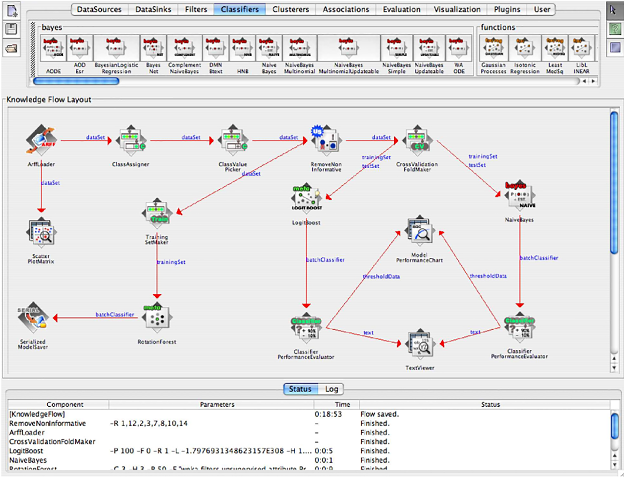
Figure A1: The WEKA Knowledge Flow user interface
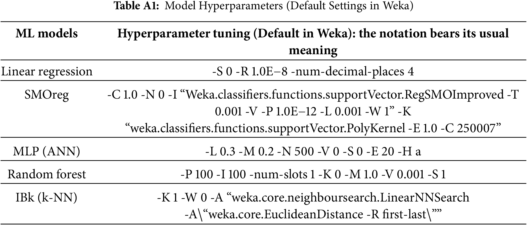
Hyperparameter tuning of the models
Table A1 shows the machine learning algorithms evaluated using their default hyperparameters as configured in the Weka software. No manual tuning or optimization was performed. Notation for parameters and performance metrics adheres to conventional usage in the machine learning literature. This table lists the default and optimized parameter settings for all the machine-learning models provided by Weka in this study. Table A1 presents each parameter’s symbolic notation, default value, and role during model training.
References
1. Sohani A, Sayyaadi H, Miremadi SR, Samiezadeh S, Doranehgard MH. Thermo-electro-environmental analysis of a photovoltaic solar panel using machine learning and real-time data for smart and sustainable energy generation. J Clean Prod. 2022;353:131611. doi:10.1016/j.jclepro.2022.131611. [Google Scholar] [CrossRef]
2. Sohani A, Sayyaadi H, Cornaro C, Shahverdian MH, Pierro M, Moser D, et al. Using machine learning in photovoltaics to create smarter and cleaner energy generation systems: a comprehensive review. J Clean Prod. 2022;364(7):132701. doi:10.1016/j.jclepro.2022.132701. [Google Scholar] [CrossRef]
3. Didavi KBA, Agbokpanzo RG, Agbomahena BM. LSTM and XGBoost models for 24-h ahead forecast of PV power from direct irradiation. Renew Energy Res Appl. 2024;5(2):229–41. [Google Scholar]
4. Banik R, Biswas A. Improving solar PV prediction performance with RF-CatBoost ensemble: a robust and complementary approach. Renew Energy Focus. 2023;46(11):207–21. doi:10.1016/j.ref.2023.06.009. [Google Scholar] [CrossRef]
5. Imam AA, Abusorrah A, Seedahmed MM, Marzband M. Accurate forecasting of global horizontal irradiance in Saudi Arabia: a comparative study of machine learning predictive models and feature selection techniques. Mathematics. 2024;12(16):2600. doi:10.3390/math12162600. [Google Scholar] [CrossRef]
6. Salimans T, Kingma DP. Weight normalization: a simple reparameterization to accelerate training of deep neural networks. Adv Neural Inf Process Syst. 2016;29. [Google Scholar]
7. Prusa J, Khoshgoftaar TM, Seliya N, editors. The effect of dataset size on training tweet sentiment classifiers. In: Proceedings of the 2015 IEEE 14th International Conference on Machine Learning and Applications (ICMLA); 2015 Dec 9–11; Miami, FL, USA. Piscataway, NJ, USA: IEEE; 2015. p. 96–102. [Google Scholar]
8. Liu H, Dougherty ER, Dy JG, Torkkola K, Tuv E, Peng H, et al. Evolving feature selection. IEEE Intell Syst. 2005;20(6):64–76. doi:10.1109/mis.2005.105. [Google Scholar] [CrossRef]
9. Dris AB, Alzakari N, Kurdi H. A systematic approach to identify an appropriate classifier for limited-sized data sets. In: Proceedings of the 2019 International Symposium on Networks, Computers and Communications (ISNCC); 2019 Jun 18–20; Istanbul, Turkey. Piscataway, NJ, USA: IEEE; 2019. p. 1–6. [Google Scholar]
10. Marion B, Deceglie MG, Silverman TJ. Analysis of measured photovoltaic module performance for Florida, Oregon, and Colorado locations. Sol Energy. 2014;110:736–44. doi:10.1016/j.solener.2014.10.017. [Google Scholar] [CrossRef]
11. Hall M, Frank E, Holmes G, Pfahringer B, Reutemann P, Witten IH. The WEKA data mining software: an update. ACM SIGKDD Explor Newsl. 2009;11(1):10–8. doi:10.1145/1656274.1656278. [Google Scholar] [CrossRef]
12. Gyeltshen S, Hayashi K, Tao L, Dem P. Statistical evaluation of a diversified surface solar irradiation data repository and forecasting using a recurrent neural network-hybrid model: a case study in Bhutan. Renew Energy. 2025;245(7):122706. doi:10.1016/j.renene.2025.122706. [Google Scholar] [CrossRef]
13. Kavitha S, Varuna S, Ramya R, editors. A comparative analysis on linear regression and support vector regression. In: Proceedings of the 2016 online international conference on green engineering and technologies (IC-GET); 2016 Nov 19; Coimbatore, India. Piscataway, NJ, USA: IEEE; 2016. p. 1–5. [Google Scholar]
14. Chieu TQ, Thao NTP, Thi Hue D, Huong NTT. Prediction of the water level at the Kien Giang River based on regression techniques. River. 2024;3(1):59–68. doi:10.1002/rvr2.71. [Google Scholar] [CrossRef]
15. Singh B, Sihag P, Singh K. Modelling of impact of water quality on infiltration rate of soil by random forest regression. Model Earth Syst Environ. 2017;3(3):999–1004. doi:10.1007/s40808-017-0347-3. [Google Scholar] [CrossRef]
16. Steinbach M, Tan P-N. kNN: k-nearest neighbors. In: The top ten algorithms in data mining. Oxfordshire, UK: Chapman and Hall/CRC; 2009. p. 165–76. [Google Scholar]
17. Asuero AG, Sayago A, González A. The correlation coefficient: an overview. Crit Rev Anal Chem. 2006;36(1):41–59. [Google Scholar]
18. Hodson TO. Root mean square error (RMSE) or mean absolute error (MAEwhen to use them or not. Geosci Model Dev Discuss. 2022;2022(14):1–10. doi:10.5194/gmd-15-5481-2022. [Google Scholar] [CrossRef]
19. Jebli I, Belouadha F-Z, Kabbaj MI, Tilioua A. Prediction of solar energy guided by person correlation using machine learning. Energy. 2021;224(11):120109. doi:10.1016/j.energy.2021.120109. [Google Scholar] [CrossRef]
Cite This Article
 Copyright © 2025 The Author(s). Published by Tech Science Press.
This work is licensed under a Creative Commons Attribution 4.0 International License , which permits unrestricted use, distribution, and reproduction in any medium, provided the original work is properly cited.
 Downloads
 Citation Tools