
 Login
Login Register
 Submit a Paper
 Propose a Special lssue
 Open Access
ARTICLE
Low-Carbon Operational Optimization of Integrated Electricity-Heat-Gas Systems Considering Regulation Capability
1 State Grid Jibei Electric Power Co., Ltd. Economic and Technical Research Institute, Beijing, China
2 State Grid Jibei Electric Power Co., Ltd., Beijing, China
3 Beijing Bowang Huake Technology Co., Ltd., Beijing, China
4 School of Economics and Management, North China Electric Power University, Beijing, China
* Corresponding Author: Yan Lu. Email:
(This article belongs to the Special Issue: Advanced Analytics on Energy Systems)
Energy Engineering 2026, 123(11), 22 https://doi.org/10.32604/ee.2026.067612
Received 07 May 2025; Accepted 20 June 2025; Issue published 24 September 2026
 View Full Text
 Download PDF
Abstract
To promote the consumption of new energy sources such as wind and solar power and to achieve multi-energy and multi-system coupling, this paper proposes a low-carbon operation optimization strategy for the Electric-Heat-Gas Coupling System (EHGCS) that incorporates regulation capabilities. First, the operational framework of the EHGCS was designed, and an equipment output model was developed, taking into account the dynamic efficiency of electrolytic cells and the delayed response characteristics of hydrogen fuel cells. Next, a regulation capability model and a dynamic regulation price model were proposed for the coupling of subsystems involving electrical, thermal, and gas energy across multiple systems. Subsequently, the correlation between energy market prices and carbon market prices was analyzed using the kernel density copula method, which informed the development of a low-carbon operation optimization model for the EHGCS. This model aims to maximize both net income and clean energy consumption. A numerical analysis was then conducted through a case study of a specific park. The results demonstrated that ignoring the dynamic efficiency of electrolytic cells increases the operating cost of the EHGCS by 5.9% while neglecting the delayed response characteristics of hydrogen fuel cells raises the system’s uncertainty cost by 3.7%. Additionally, considering the flexible adjustment capability of the electric-thermal-gas multi-system reduces user energy costs by 2169.75 CNY and boosts clean energy consumption by 8.22%. Incorporating dynamic price adjustments further enhances the system’s dynamic regulation capacity. Finally, the application of the kernel density copula method accurately captures the correlation between energy and carbon markets, resulting in a 23.17% increase in EHGCS net income.Keywords
As of 2024, China’s renewable energy generation reached approximately 3.47 trillion kilowatt-hours, accounting for around 35% of the country’s total electricity production [1]. With the development of new energy such as wind and solar energy, limited by location factors, wind and solar resources are mainly concentrated in the three northern regions. The load demand is concentrated in the coastal areas of central and southeastern China, leading to difficulties in consumption and prominent issues of wind and solar power abandonment [2]. At the end of 2024, the National Development and Reform Commission and the National Energy Administration jointly issued the Implementation Plan for the Special Action on Enhancing Power System Regulation Capability (2025–2027) [3]. The plan outlines a series of key tasks aimed at improving the planning and development of regulation resources, optimizing their dispatch mechanisms, and refining their participation in market-based systems. By strengthening the regulatory flexibility and dispatchability of the power system, the initiative seeks to support the effective integration of over 200 GW of newly installed renewable energy capacity annually during 2025–2027. It sets a clear target for 2027: the national renewable energy utilization rate shall not fall below 90%. However, relying solely on the power system’s inherent regulation capability is insufficient to achieve the local integration of large-scale renewable energy. It is therefore imperative to establish a multi-energy system encompassing diverse energy forms, enabling coordinated operation between the power system and other energy infrastructures [4]. Hydrogen, as a clean and efficient secondary energy source, offers high energy density, large capacity, long lifespan, and ease of storage and transmission. By coupling and complementing different forms of energy, such as electricity, heat, cold, and gas—a hydrogen-containing coupled energy system can be established. This system can significantly improve energy utilization efficiency and promote clean energy consumption [5]. Consequently, coupling systems integrating multiple energy sources like electricity, heat, and gas have become a key focus of research.
In the electric-thermal-gas coupling system, electrolytic cells and hydrogen fuel cells serve as key conversion and coupling equipment, necessitating detailed research on their operation. Regarding electrolytic cells, Ma et al. [6] constructed a physical model of a PEM electrolyzer by simulating the performance of coupled thermal fluid, matter transfer and electrochemical processes. Dang et al. [7] compared and summarizes the theoretical mathematical models of PEM electrolyzers and other types of electrolyzers. It analyzes the impact of various control strategies and shutdown procedures on transient behavior, and explains the transient phenomena observed during the shutdown process based on the theoretical principles of hydrogen-oxygen fuel cells. Frensch et al. [8] provided impedance spectra and current-voltage characteristic curves of electrolytic cells under various current densities and over time, indicating that the voltage efficiency of electrolytic cells continuously decreases with operating time.
Concerning hydrogen fuel cells, Yang et al. [9] proposed accounting for the cogeneration characteristics of hydrogen fuel cells to mitigate the limitations of cogeneration units whose electricity output is heat-determined. Han et al. [10] highlighted a significant response delay when hydrogen fuel cells start at room temperature. From this literature review, it can be concluded that the efficiency of electrolytic cells dynamically varies with external conditions and component aging, while hydrogen fuel cells exhibit delayed response characteristics. However, existing research on optimizing hydrogen-containing energy systems typically assumes a fixed efficiency for electrolytic cells, while allowing hydrogen fuel cells to respond in real-time, thus neglecting both the dynamic efficiency changes of electrolytic cells and the delayed response of hydrogen fuel cells.
With the increasing coupling characteristics of multiple loads such as electricity, heat, cooling, and gas, traditional demand response has evolved into a comprehensive demand response. Dong et al. [11,12] developed an operational optimization model for comprehensive energy systems considering a single demand response type. Building upon this, Wang et al. [13] proposes a synergistic planning method for an integrated energy system with hydrogen storage taking into account the coupled use of electric-thermal energy, which effectively reduces the system carbon emission and improves the comprehensive energy efficiency level. Li et al. [14] established a demand response model incorporating both price-based and incentive-based loads, analyzing the behavioral characteristics of residential participants in demand response programs.
Existing demand response research effectively models various types of responses but still has two main limitations. First, it primarily focuses on electrical and thermal energy systems without simultaneously considering the regulatory capabilities of electrical, thermal, and gas energy systems. In hydrogen energy systems, flexibility arises from the integration of hydrogen fuel cells, electrolytic cells, and hydrogen blending pipelines, allowing the system to act as a schedulable resource. Second, demand response pricing generally adopts fixed call prices, which inadequately reflect the system’s willingness to adjust the demand scale.
Optimizing operation to maximize the benefits of electric, thermal, and gas coupling systems remains a key research area. Wang et al. [15,16] studied a coupled system incorporating renewable distributed generation and multiple energy loads. To mitigate uncertainty in renewable output, they developed an operational optimization model for participation in day-ahead and real-time electricity markets. Extending beyond single-market participation, Wang et al. [17] proposed a day-ahead economic scheduling model for a Renewable Energy-dominated Hybrid Integrated Electricity-Hydrogen Energy System (REHIES), aiming to accommodate market demand through enhanced coordination between electricity and hydrogen energy. Li et al. [18] proposed an innovative Electro-Hydrogen Regional Energy System and developed a cost-minimizing scheduling model that incorporates a stepped carbon pricing mechanism and the operational characteristics of hydrogen fuel cells, aiming to enhance system flexibility and renewable energy utilization.
While existing research can optimize system operation across multiple markets through multi-energy coupling, it generally fails to consider the coupling correlation between prices across these markets.
1.3 Contributions of the Paper
On the basis of the above research, this article conducts a low-carbon operation optimization study of the electric-heat-gas coupling system (EHGCS) that incorporates regulation capability. Compared with existing studies, this article presents the following innovations:
- (1)Device-Level Dynamic Modeling
Unlike previous works that assume constant efficiency or instantaneous response of hydrogen-related components, this study incorporates a dynamic hydrogen production efficiency model for proton exchange membrane (PEM) electrolyzers, accounting for environmental variations and degradation over time. Additionally, a delay-response penalty cost is introduced for hydrogen fuel cells, reflecting the temporal inertia in electricity-to-gas-to-electricity conversion. This dual modeling approach enhances the accuracy and responsiveness of system-level optimization.
- (2)Coupled Regulation and Pricing Mechanism
While most prior studies focus on single energy carriers or assume static regulation capacity, this work constructs a regulation capability model that captures the coupling effects among electric, thermal, and gas subsystems. By integrating the operational flexibility of hydrogen pipelines, electrolyzers, and fuel cells, the model enables a more comprehensive and realistic quantification of system regulation potential. Furthermore, a dynamic pricing mechanism based on multi-energy contribution coefficients is proposed to reflect real-time supply–demand interactions, which has been largely overlooked in existing literature.
- (3)Market-Aware Optimization with Price Dependency
Existing models often treat energy and carbon markets independently or adopt simplistic correlation assumptions. In contrast, this study applies a kernel density estimation–copula approach to quantify nonlinear dependencies between electricity and carbon prices. This allows the optimization framework to dynamically respond to market fluctuations and improve resource allocation under joint market signals, leading to a more robust and profitable low-carbon operation strategy.
The remainder of this paper is organized as follows. Section 2 presents the design of the operational framework for the EHGCS and constructs the equipment output model, as well as a regulation capability model that accounts for the coupling of electrical, thermal, and gas energy subsystems across multiple systems. Section 3 builds upon this foundation to develop a low-carbon operation optimization model based on the kernel density copula method, with the objectives of maximizing EHGCS net profit and clean energy consumption. Section 4 provides a numerical analysis using a case study of a specific park, offering practical insights for optimizing the operation of multi-energy coupling systems.
2 EHGCS Framework Design and Output Modeling
2.1 System Operation Framework
The EHGCS described in this article consists of coupled subsystems of electrical energy, thermal energy, and gas energy. The electricity subsystem meets load demand through wind power generation, photovoltaic power generation, batteries, and hydrogen fuel cells. The gas energy subsystem comprises two types: hydrogen energy and natural gas. Hydrogen energy is primarily supplied by electrolyzer units and hydrogen storage tanks to satisfy hydrogen load demand. Natural gas is partially produced via carbon capture equipment that captures carbon dioxide from gas boilers and hydrogen from hydrogen storage tanks. This captured gas is converted into natural gas through methanation equipment to meet natural gas load demand. Additionally, to balance economic and low-carbon objectives, surplus hydrogen energy can be transported via natural gas pipelines to natural gas plants and hydrogen refueling stations in other regions. The heat energy subsystem supplies thermal load by utilizing waste heat generated from electrolyzers, hydrogen fuel cells, and gas boilers. The overall system framework is illustrated in Fig. 1.
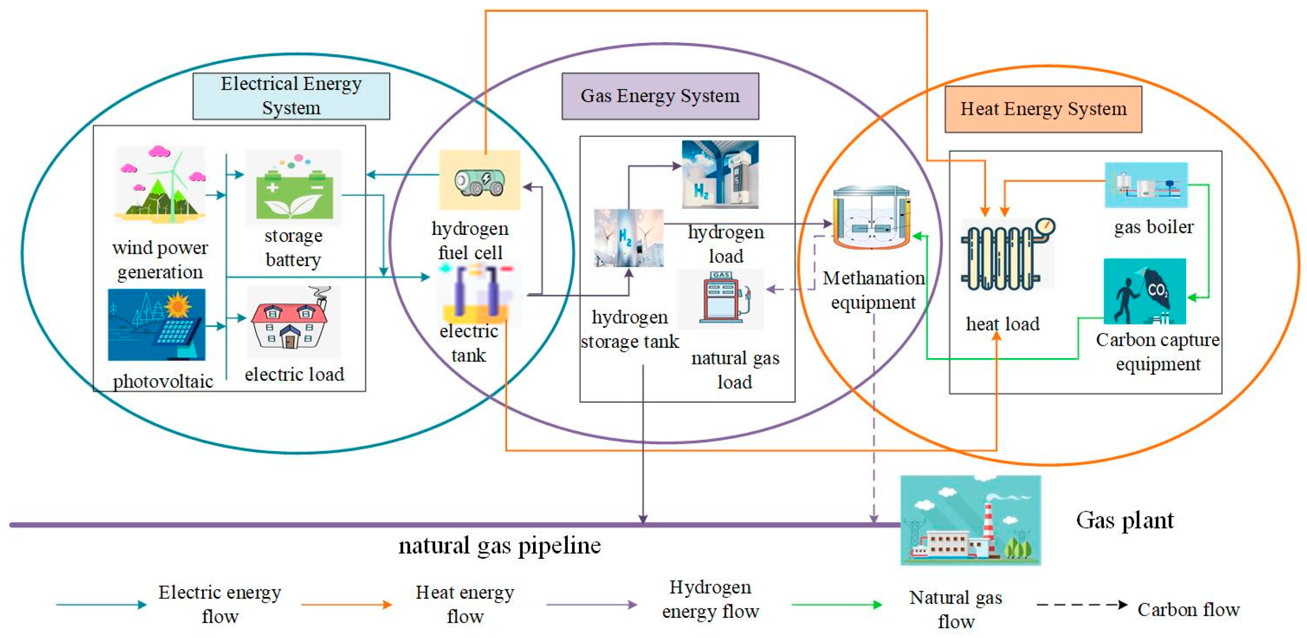
Figure 1: System coupling framework.
Based on the system coupling framework, model the equipment involved in the electric, gas, and heat energy subsystems.
2.2.1 Electric Energy Subsystem
- (1)Wind power and photovoltaic
The output of wind power generation in the electrical energy subsystem is closely related to wind speed, while photovoltaic power generation output depends on light intensity. The Weibull distribution and Beta distribution are commonly used to model the outputs of wind power and photovoltaic power, respectively [19]. This is expressed as shown in Eq. (1):
- (2)Battery (BA)
The power state values of the battery in the electric energy system should remain equal throughout a cycle of use, as shown in Eq. (2). The operating life of a battery is an important parameter, and its operating life model is specifically shown in Eq. (3):
- (3)Hydrogen fuel cell
PEM hydrogen fuel cells offer advantages such as cleanliness, zero pollution, and high energy conversion efficiency. Therefore, in this article, the term “hydrogen fuel cells” specifically refers to PEM hydrogen fuel cells. When the fuel cell parameters and external environment remain constant, the power output can be indirectly controlled by adjusting the hydrogen input rate and the circulating water flow rate. The output power and efficiency of hydrogen fuel cells are detailed in Eq. (4):
PEM hydrogen fuel cells require a heating process of several tens of minutes from start-up to optimal operating state, with delayed response characteristics. The specific delay coefficient is shown in Eq. (6):
- (1)Electrolytic cell
The application of PEM electrolytic cells is relatively mature; therefore, the electrolytic cell discussed in this article refers to a PEM electrolytic cell. Hydrogen production depends on the efficiency of the electrolytic cell and the electric-to-hydrogen conversion efficiency. The efficiency of the electrolytic cell is the product of voltage efficiency and current efficiency, as expressed in Eq. (7):
After long-term operation, PEM electrolytic cells experience component aging and thinning of the PEM. This leads to increased hydrogen permeation and a decline in dynamic current efficiency. Additionally, electrolyte conductivity decreases, causing a rise in Ohmic resistance and an increase in Ohmic voltage. Consequently, the dynamic voltage efficiency of the electrolytic cell decreases as operating time increases. These dynamic changes in current efficiency and voltage efficiency together cause the overall efficiency of the electrolytic cell to vary over time, as described in Eq. (8):
- (2)Compressed hydrogen storage system
The compressed hydrogen system consists of a compressor and a hydrogen storage tank. Its operating principle involves compressing hydrogen produced by the electrolytic cell and storing it in the hydrogen storage tank to meet hydrogen demand. However, the compression process consumes power, which is specifically described in Eq. (9):
Hydrogen, having the smallest relative molecular weight, is more prone to expansion under high pressure compared to other gases. Therefore, accurately characterizing the pressure within hydrogen storage tanks is essential. The relationship between pressure and hydrogen storage capacity is expressed in Eq. (10):
The temporal relationship between the hydrogen storage capacities of two adjacent hydrogen storage tanks is expressed in Eq. (11):
- (3)Methanation device
In the methanation unit, hydrogen gas produced by the electrolyzer or released from the hydrogen storage tank reacts with carbon dioxide captured by the carbon capture equipment to generate natural gas under the action of a catalyst. The consumption of hydrogen and carbon dioxide, as well as the production of natural gas in the methanation unit, are detailed in Eq. (12):
- (4)Hydrogen doped natural gas pipeline
Hydrogen-doped natural gas pipelines enable long-distance hydrogen transport without additional investment. Assuming hydrogen is uniformly distributed within the natural gas pipeline, the specific ratio of hydrogen to the calorific value of hydrogen-doped natural gas is expressed in Eq. (13):
- (1)Waste heat utilization
Waste heat utilization refers to recovering waste heat from flue gases of electrolytic cells and hydrogen fuel cells using waste heat recovery devices to meet users’ thermal load demands. The specific amount of waste heat utilized is shown in Eq. (14):
- (2)Gas boiler
The gas boiler generates heat energy by consuming natural gas produced by the methanation equipment. The heat output of the gas boiler depends on the natural gas consumption, the boiler’s efficiency, and the calorific value of the natural gas, as shown in Eq. (15):
- (3)Carbon capture equipment
The carbon capture equipment absorbs carbon dioxide emitted by gas boilers and supplies it to the methanation units for further use. The amount of carbon dioxide captured by the equipment is expressed in Eq. (16):
The energy consumption of the carbon capture system includes both operational and fixed energy consumption, as shown in Eq. (17):
3 Analysis of EHGCS Flexible Regulation Capability
The EHGCS involves multiple energy flows and loads. This article analyzes the flexible regulation capabilities of the electric, heat, and gas energy subsystems, as well as the overall coupled system.
3.1 Electric Energy Subsystem Regulation Capability
In the energy subsystems, regulation capability varies due to users’ subjective willingness and the price difference between peak and off-peak periods. When the price difference is below a certain threshold, users show low enthusiasm for participating in regulation, creating a “dead zone” of regulation participation. Conversely, if the price difference is too large, users tend to reach a saturation point to maintain a comfortable energy consumption experience, resulting in a “saturation zone” for participation. Additionally, the greater the users’ willingness to participate, the higher the likelihood of their engagement in regulation. Based on a combination of logistic and trapezoidal membership functions, a regulation capability model for the electric energy subsystem is constructed. The principle of this model is illustrated in Fig. 2:
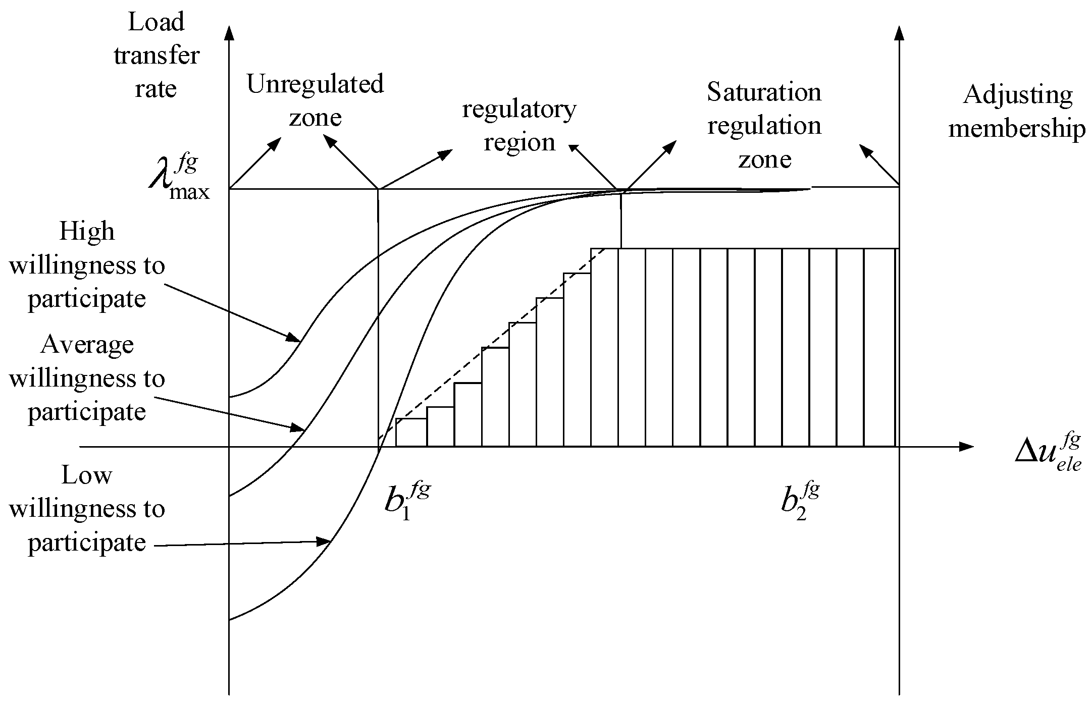
Figure 2: Principle diagram of electrical energy subsystem regulation capability.
To account for user participation willingness, the average load transfer rate is calculated based on the load transfer rates of users with high and low willingness to participate. This average rate serves as a measure of the regulation capability of the energy subsystem. Using peak and valley periods as an example, the average load transfer rate during these periods is given by Eq. (18):
Using Eq. (18), the load transfer rates for the peak and valley periods are calculated as a and b, respectively. Based on these values, the regulation capability of the electrical energy subsystem is expressed in Eq. (19):
3.2 Heat Energy Subsystem Regulation Capability
Because indoor temperature can fluctuate within a certain range without compromising user comfort, the thermal load can be adjusted accordingly while still meeting comfort requirements. The magnitude of this adjustable thermal load represents the regulation capability of the thermal energy subsystem. The user’s indoor temperature model is shown in Eq. (20):
Based on Eq. (20), the user’s heat load model is obtained as shown in Eq. (21):
Let the acceptable range of indoor temperature variation for users be
3.3 Gas Energy Subsystem Regulation Capability
To capture the time-delay characteristics inherent in the electricity-to-gas and gas-to-electricity conversion processes, this study incorporates a response lag parameter within the hydrogen fuel cell modeling. This approach reflects the dynamic delays associated with hydrogen production via electrolysis, storage, and reconversion to electricity. It enhances the representation of the gas subsystem’s dynamic behavior and allows for a more realistic assessment of its temporal effectiveness and stability in supporting power system regulation. The gas energy subsystem can achieve spatial energy transfer via hydrogen-doped natural gas pipelines during periods of low energy consumption. The volume of this spatial transfer represents the regulation capacity of the gas energy subsystem. This regulation capability depends on both the hydrogen blending capacity of the natural gas pipeline and the hydrogen production capacity of the electrolytic cell. The regulation capability model of the gas energy subsystem is detailed in Eq. (23):
3.4 Multi-System Coupling Regulation Capability
The EHGCS enables the conversion between electricity, gas, and heat. Therefore, beyond considering the transfer capabilities of each individual subsystem, it also accounts for the substitutable regulation capability arising from multi-system coupling. This mainly includes electricity-gas load substitution and gas-heat load substitution, as shown in Eqs. (24) and (25):
4 Optimization Modeling of EHGCS Low-Carbon Operation Considering Multi-System Regulation
After satisfying its internal diversified load demands, the EHGCS can participate in the joint energy-carbon market. When the system’s free carbon quota exceeds its actual carbon emissions, EHGCS can sell the surplus carbon allowances in the carbon market. Conversely, if emissions exceed the quota, it must purchase additional allowances. Similarly, when EHGCS’s energy supply surpasses demand, it can sell the excess energy in the energy market; otherwise, it can buy the shortfall energy to meet its needs. This interaction forms the joint energy-carbon market. The operating principle of EHGCS’s market participation is illustrated in Fig. 3.
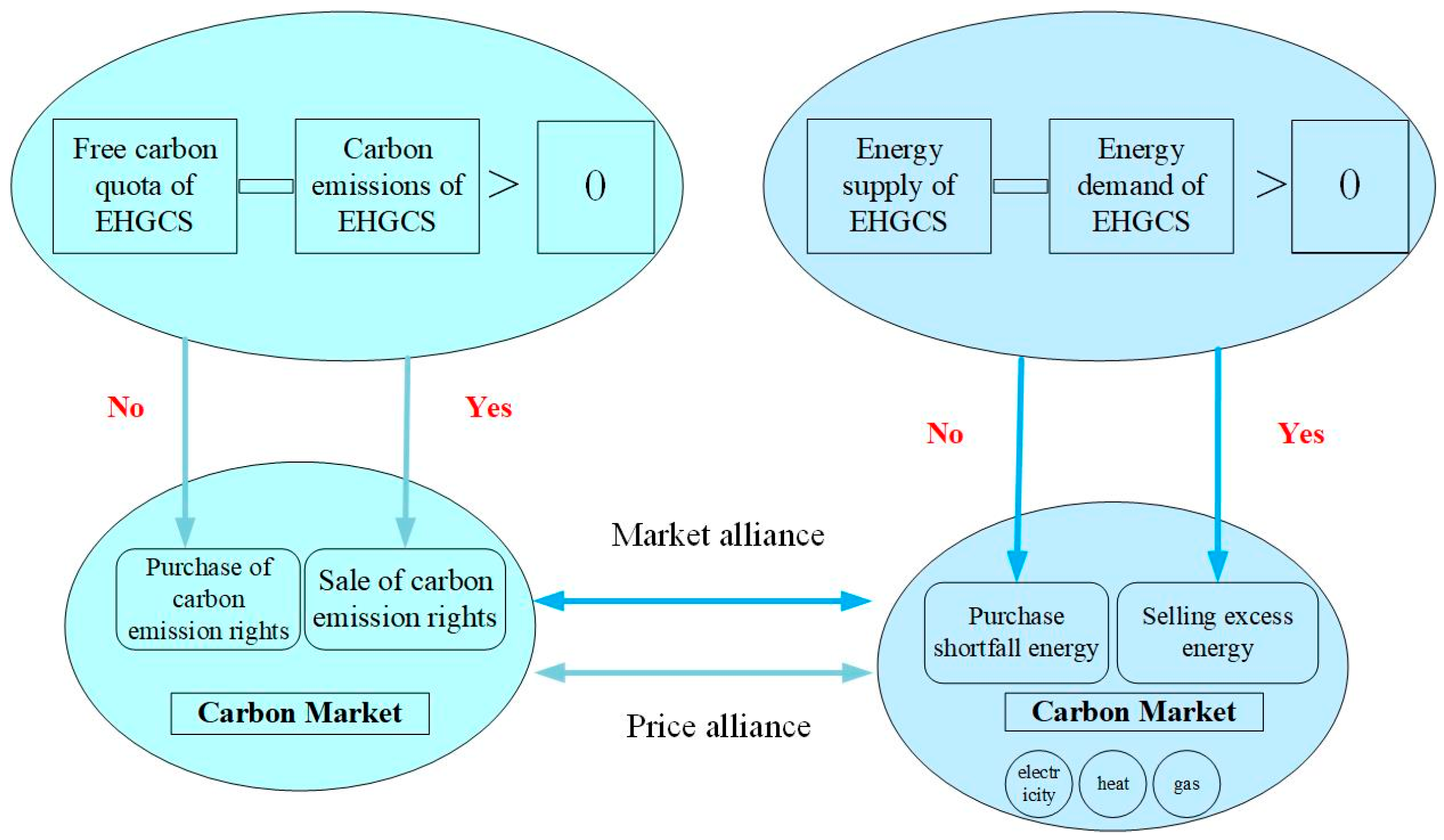
Figure 3: EHGCS participation in market operation schematic.
To balance the economic and environmental benefits of EHGCS, the objective function aims to maximize both the system’s net profit and clean energy consumption.
EHGCS net revenue is defined as the difference between total revenue and total cost, as shown in Eq. (26):
- (1)Total revenue
The total revenue of EHGCS includes internal energy sales revenue
The specific internal sales revenue is shown in Eq. (28):
The specific gas transmission benefits of hydrogen blending pipelines are shown in Eq. (29):
The benefits of participating in the market are shown in Eq. (30):
When the carbon market price rises, EHGCS tends to reduce carbon emissions by lowering gas boiler output, which decreases the system’s energy supply. If the system is in a shortage state, this shortage worsens, increasing market demand and causing energy prices to drop. Conversely, if the system has excess supply, the reduction causes energy prices to rise. This demonstrates a correlation between carbon market prices and energy market prices. In this paper, the kernel density estimation method-Copula method is used to characterize the nonlinear correlation between carbon market price and energy market (price). Firstly, the marginal distribution functions of various energy prices and carbon prices are obtained through the kernel density estimation method, so as to preserve their actual distribution characteristics; subsequently, the Copula function is introduced to construct a joint distribution model to establish the dependence structure between different energy prices and carbon prices. This joint distribution is used to simulate the joint fluctuation of various price variables in the scenario generation stage, realizing the multi-scenario inputs under the price linkage between carbon and energy markets. On this basis, the generated price scenarios are embedded into the EHGCS low-carbon operation optimization model, which is used to calculate the net benefit and uncertainty cost under multiple scenarios, and to control the tail risk through the CVaR indicator, so as to improve the model’s adaptability and robustness to market fluctuations. The historical sample vectors of carbon emission rights, electricity, hydrogen, natural gas, and thermal energy prices as
- (2)Total cost
The total cost of EHGCS comprises of system uncertainty cost
In this study, uncertainty costs are characterized using Conditional Value-at-Risk (CVaR), a widely adopted risk measure that effectively captures the impact of extreme deviations caused by load fluctuations and renewable generation uncertainty. As a second-order risk metric, CVaR incorporates tail risks into the objective function by constraining the expected loss beyond a specified confidence level, thereby enhancing the model’s robustness and its ability to manage volatility. This enables the proposed optimization framework to explicitly account for the stochastic nature of renewable energy and demand. The detailed formulation can be found in reference [21]. The specific operating cost of the unit is shown in Eq. (33):
When the system experiences a significant energy demand shortage, the adjustment price should increase accordingly. To reflect this, a contribution coefficient is incorporated into the adjustment cost to form a dynamic adjustment price, as shown in Eq. (34):
The delayed response cost of hydrogen fuel cells is specifically represented in Eq. (35):
The specific market operating costs are shown in Eq. (36):
4.1.2 Maximizing Clean Energy Consumption Rate
The maximization of the clean energy consumption rate aims to maximize the absorption of wind and solar power output within the system, as shown in Eq. (37):
The operational constraints of EHGCS primarily include unit operation constraints, power balance constraints, regulation capacity constraints, and transmission channel constraints.
4.2.1 Unit Operation Constraints
The primary constraint on unit operation is that the output of each piece of equipment must remain within its specified upper and lower limits, as shown in Eq. (38).
4.2.2 Regulatory Ability Constraints
The regulation capacity constraint refers to the requirement that the actual regulation performed by multiple subsystems must not exceed their respective maximum regulation capacities, as shown in Eq. (39).
4.2.3 Transmission Channel Constraints
The transmission channel constraint refers to the upper and lower limits on both the energy exchanged between the EHGCS and the external market and the volume of hydrogen transported through hydrogen-doped natural gas pipelines, as shown in Eq. (40).
4.2.4 Power Balance Constraint
Power balance constraint refers to the power balance of the electrical, thermal, and gas subsystems, as shown in Eq. (41):
This study conducts a simulation analysis based on a typical electric-thermal-gas coupling park in China, using a 24-h period on a representative day. In the simulation, it is assumed that a gas boiler emits 1.023 kg of CO2 for every 1 kWh of thermal energy produced, with a free carbon quota set at 0.5 kg/kWh. The operational cost of the carbon capture equipment is set at 57.18 CNY per ton of CO2 captured. The operating parameters for the remaining types of equipment are detailed in Table 1 [22,23].
Table 1: Operating parameters of other types of equipment.
| Parameter | Value | Parameter | Value | Parameter | Value | Parameter | Value |
|---|---|---|---|---|---|---|---|
| 55% | 24.18 kg/kWh | 70% | 0.0243 kg/kWh | ||||
| 35% | 15% | 90% | 0.7 | ||||
| 90% | 90% | 90% | 90% | ||||
| 4.338 ∗ 108 J/kg | 1.4 ∗ 108 J/kg | 5.071 ∗ 107 J/kg | 0.23 MWh/t | ||||
| 81.8% | 0.5034 CNY/kWh | 0.839 CNY/kWh |
The operating costs of various equipment are shown in Table 2:
Table 2: Cost parameters for other types of equipment.
| Parameter | Value | Parameter | Value | Parameter | Value | Parameter | Value |
|---|---|---|---|---|---|---|---|
| 0.01 CNY/kWh | 0.04 CNY/kWh | 0.009 CNY/kWh | 0.062 CNY/kWh | ||||
| 0.5 CNY/m3 | 0.07 CNY/kWh | 0.01 CNY/kg | 0.09 CNY/kWh |
The upper and lower limits, energy interaction limits, and transmission channels of various devices are shown in Table 3 [24]:
Table 3: Limit parameter.
| Parameter | Value | Parameter | Value | Parameter | Value | Parameter | Value |
|---|---|---|---|---|---|---|---|
| 0 kW | 10,000 kW | 0 kW | 6000 kW | ||||
| −500 kW | 500 kW | −120 kg | 120 kg | ||||
| 1100 kW | 5500 kW | 0 m3 | 50 m3 | ||||
| 0 kW | 200 kW | −2500 kW | 2500 kW | ||||
| −13 kg | 13 kg | −3 m3 | 3 m3 | ||||
| −1200 kW | 1200 kW | 0 kW | 1000 kW |
Set the time of use electricity price for EHGCS to sell energy to internal users in the system, as shown in Table 4:
Table 4: Time of use electricity price for energy sales.
| Electricity Selling Price | Heat Selling Price | ||||
|---|---|---|---|---|---|
| Time | Price | Time | Price | ||
| Valley period | 1:00–7:00 22:00–24:00 | 0.502 CNY/kWh | Valley period | 1:00–7:00 22:00–24:00 | 0.107 CNY/kWh |
| Flat period | 8:00–11:00 16:00–17:00 | 0.732 CNY/kWh | Flat period | 11:00–14:00 18:00–21:00 | 0.224 CNY/kWh |
| Peak period | 12:00–15:00 18:00–21:00 | 1.216 CNY/kWh | Peak period | 8:00–10:00 15:00–17:00 | 0.325 CNY/kWh |
| Hydrogen Selling Price | Gas Selling Price | ||||
| Time | Price | Time | Price | ||
| Valley period | 5:00–9:00 22:00 | 9 CNY/kg | Valley period | 1:00–6:00 | 1.571 CNY/m3 |
| Flat period | 10:00–16:00 23:00–24:00 | 11 CNY/kg | Flat period | 11:00–13:00 18:00–20:00 22:00–24:00 | 1.933 CNY/m3 |
| Peak period | 1:00–4:00 17:00–21:00 | 13 CNY/kg | Peak period | 7:00–10:00 14:00–17:00 | 2.168 CNY/m3 |
EHGCS sells hydrogen and natural gas through hydrogen blending channels at prices shown in Table 5:
Table 5: Prices of hydrogen sales and natural gas sales in the hydrogen dopant corridor.
| Hydrogen Selling Price | Gas Selling Price | ||||
|---|---|---|---|---|---|
| Time | Price | Time | Price | ||
| Valley period | 5:00–9:00 22:00 | 10 CNY/kg | Valley period | 1:00–6:00 | 1.591 CNY/m3 |
| Flat period | 10:00–16:00 23:00–24:00 | 12 CNY/kg | Flat period | 11:00–13:00 18:00–20:00 22:00–24:00 | 1.953 CNY/m3 |
| Peak period | 1:00–4:00 17:00–21:00 | 14 CNY/kg | Peak period | 7:00–10:00 14:00–17:00 | 2.188 CNY/m3 |
After calculation, the dynamic operating efficiency of the electrolytic cell is shown in Fig. 4:
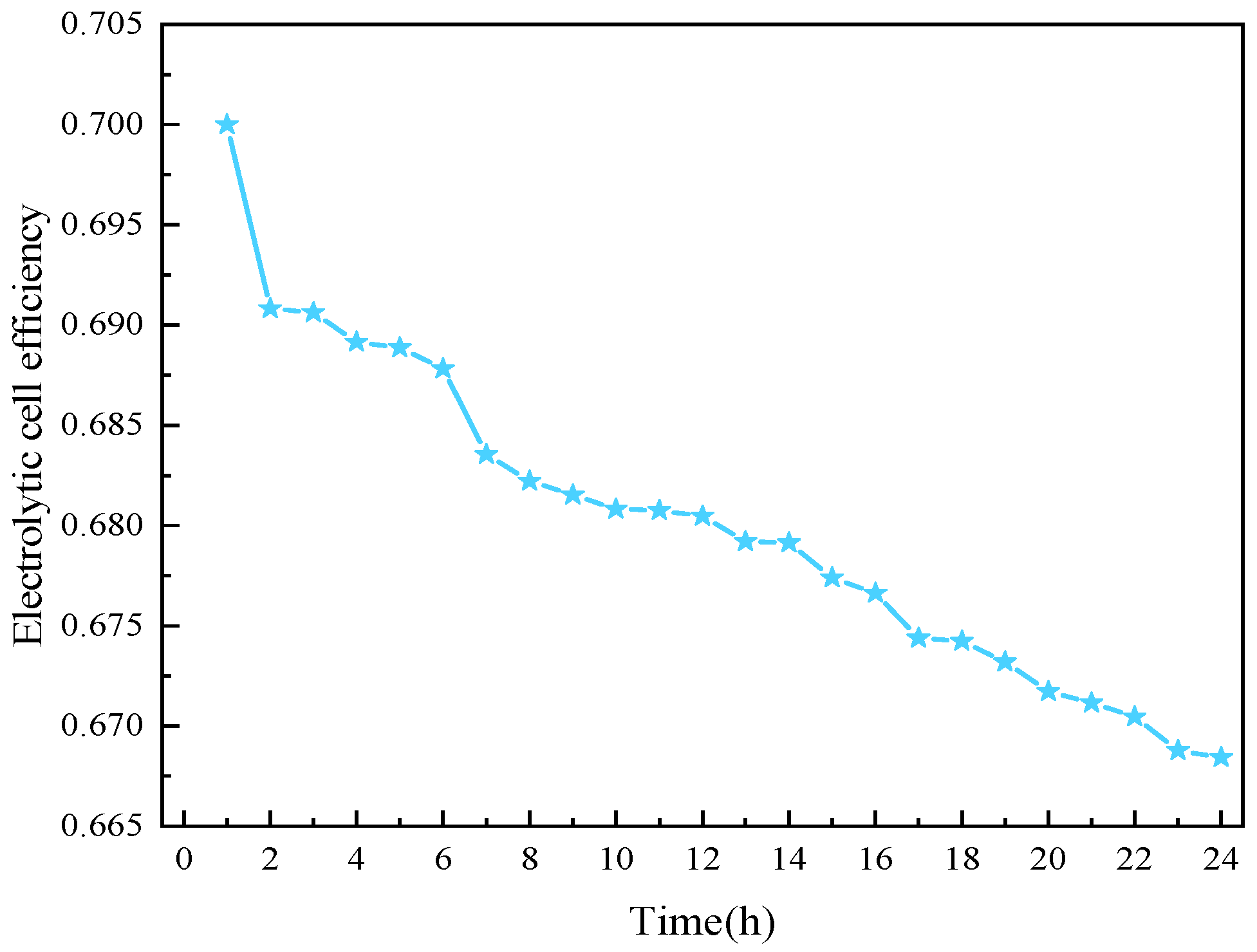
Figure 4: Dynamic operating efficiency of electrolytic cells.
The typical daily wind and solar power output and diversified load demand of EHGCS are shown in Fig. 5 and Fig. 6 [25].
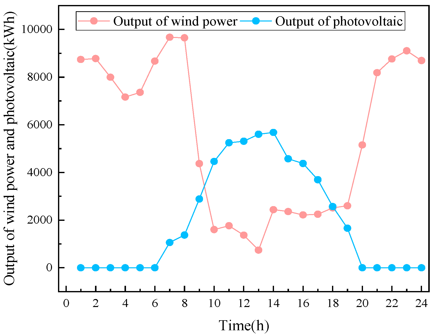
Figure 5: Wind power and photovoltaic output.
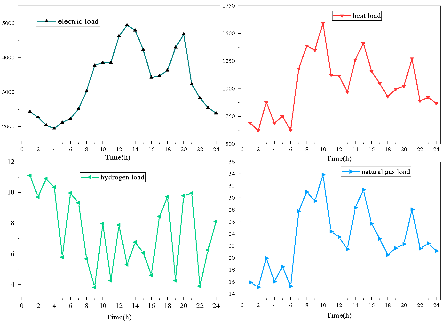
Figure 6: Multivariate load demand.
5.2.1 Analysis of EHGCS Operation Optimization Results
This section mainly provides a detailed analysis of the system output structure and various load adjustment prices.
- (1)System output structure
Based on the operational optimization model presented in Part 4, the optimization results for the electrical, thermal, hydrogen, and natural gas subsystems are illustrated in Fig. 7. Each subfigure represents the performance and coordination of key components within its respective subsystem. Fig. 7a displays the Electrical Energy Subsystem. Here, Power 1 and Power 2 represent wind and photovoltaic power generation, respectively, reflecting the system’s renewable energy inputs. Power 3 denotes interactive electricity transactions with the market, where a positive value indicates energy purchase and a negative value indicates energy sales. Power 4 is the output from hydrogen fuel cells, while Power 5 reflects battery charging and discharging (negative for charging, positive for discharging). Power 6 shows the electricity consumption by electrolytic cells, Power 7 indicates the electricity regulation amount and Power 8 accounts for energy used in carbon capture. Fig. 7b presents the Thermal Energy Subsystem. Heat 1 and Heat 2 correspond to waste heat recovery from electrolytic cells and hydrogen fuel cells, respectively. Heat 3 is thermal energy generated by gas boilers, while Heat 4 refers to interactions with the thermal energy market. Heat 5 represents thermal energy regulation. Fig. 7c illustrates the Hydrogen Energy Subsystem. Hydrogen 1 indicates hydrogen production via electrolytic cells, and Hydrogen 2 captures the charging and discharging behavior of hydrogen storage tanks (negative for charging, positive for discharging). Hydrogen 3 and Hydrogen 4 represent hydrogen consumed by methanation equipment and hydrogen fuel cells, respectively. Hydrogen 5 shows hydrogen market transactions (positive for purchasing, negative for selling), while Hydrogen 6 refers to the hydrogen energy regulation amount. Hydrogen 7 represents the transport capacity of hydrogen through hydrogen-doped natural gas pipelines. Fig. 7d covers the Natural Gas Subsystem. Natural Gas 1 represents gas production through methanation. Natural Gas 2 indicates natural gas regulation, and Natural Gas 3 shows pipeline transmission capacity. Natural Gas 4 involves market interactions (positive for purchasing, negative for selling), and Natural Gas 5 reflects gas consumption by gas boilers. It is also important to note that both battery and hydrogen storage tank operations are denoted as negative during charging (energy input/storage) and positive during discharging (energy output). Additionally, market interaction values follow a consistent convention across subsystems: positive values represent energy or resource purchases, while negative values represent sales to the market.
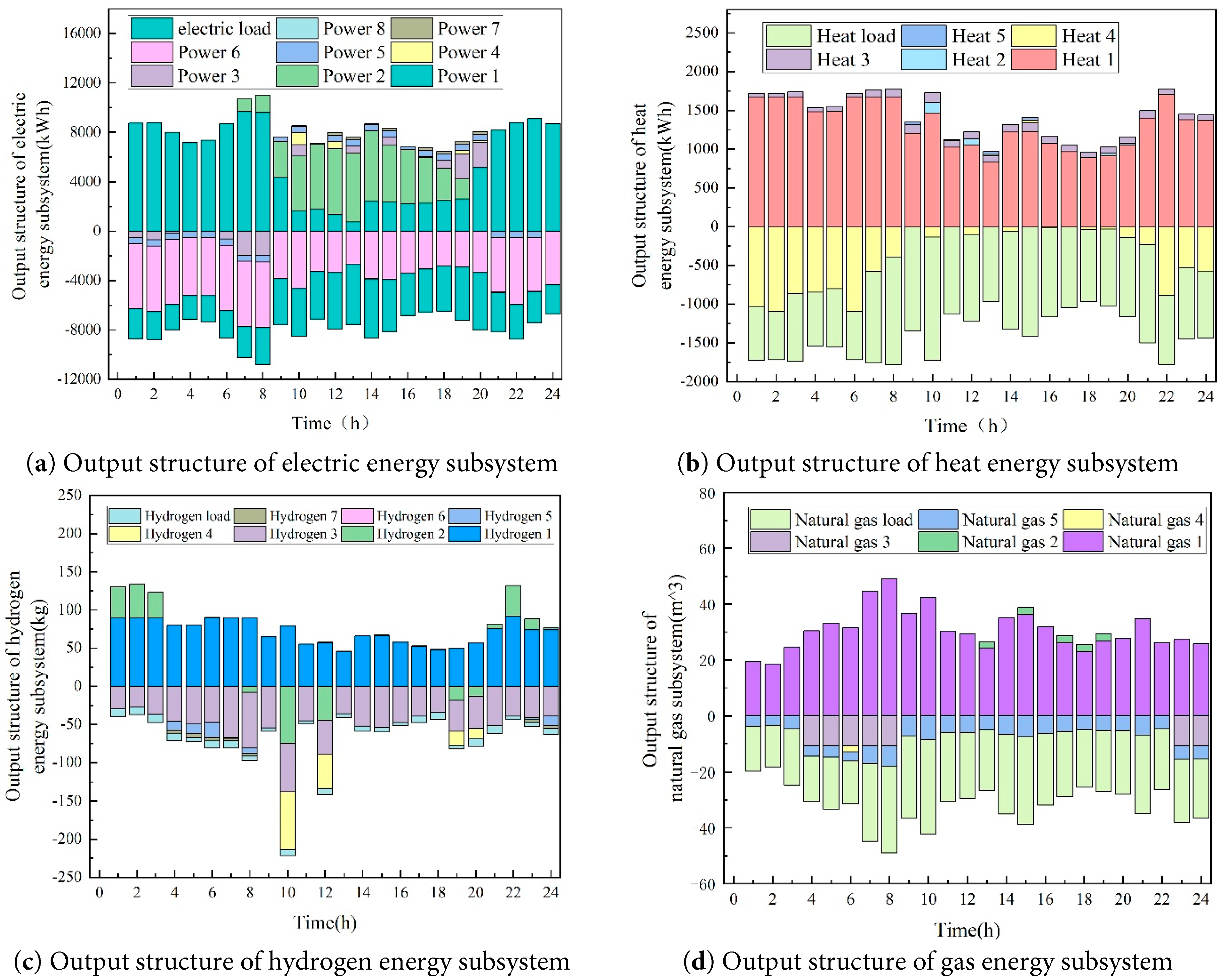
Figure 7: EHGCS operation optimization results.
From Fig. 7a, the electrical energy subsystem shows that between 1:00 and 8:00, the system generates more electricity than required to meet the user load, the electrolytic cell energy consumption, and the carbon capture energy consumption. The surplus electricity is stored in the battery until its capacity limit of 500 kW is reached at each time point. Once fully charged, any additional surplus is sold to the energy market. This strategy is employed because electricity market prices are low during this period, prompting the system to store energy for resale during peak price periods. Between 9:00 and 20:00, the system experiences an energy shortage. This deficit is mitigated through several coordinated strategies: discharging stored energy from batteries, utilizing the flexible regulation capacity of users, converting stored hydrogen into electricity via hydrogen fuel cells, and purchasing additional electricity from the market when necessary. These measures collectively help maintain energy balance and ensure system stability during peak demand periods. For example, at 17:00 and 18:00, the system bought 104.57 kWh and 687.12 kWh of electricity, respectively, due to the depletion of hydrogen reserves. Earlier, the hydrogen fuel cells had already converted 1000 kWh (at 10:00) and 596 kWh (at 12:00), exhausting the hydrogen storage capacity.
In Fig. 7b, the thermal energy subsystem relies mainly on waste heat recovery from the electrolytic cell and supplementary heat from gas boilers. At 9:00, 11:00, 13:00, and 15:00, demand peaks create thermal shortages. These are resolved by activating the adjustable thermal load of users. Fig. 7c,d highlights the hydrogen and natural gas subsystems, which are tightly coupled. From 4:00 to 8:00, the hydrogen storage tank exceeds capacity, prompting the system to transport 4 kg of hydrogen via hydrogen-doped natural gas pipelines. Any remaining hydrogen beyond the pipeline’s maximum capacity is sold to the energy market. For instance, at 4:00, after transporting 4 kg, an excess of 12.22 kg was sold, as regional gas plant prices were higher than market prices. During the peak demand period from 17:00 to 19:00, both hydrogen and natural gas regulation capacities are mobilized to address the energy shortfall.
- (1)Diversified price adjustment
Based on the dynamic adjustment price model in Eq. (33), the dynamic adjustment prices for electricity, heat, hydrogen, and natural gas are calculated and illustrated in Fig. 8.
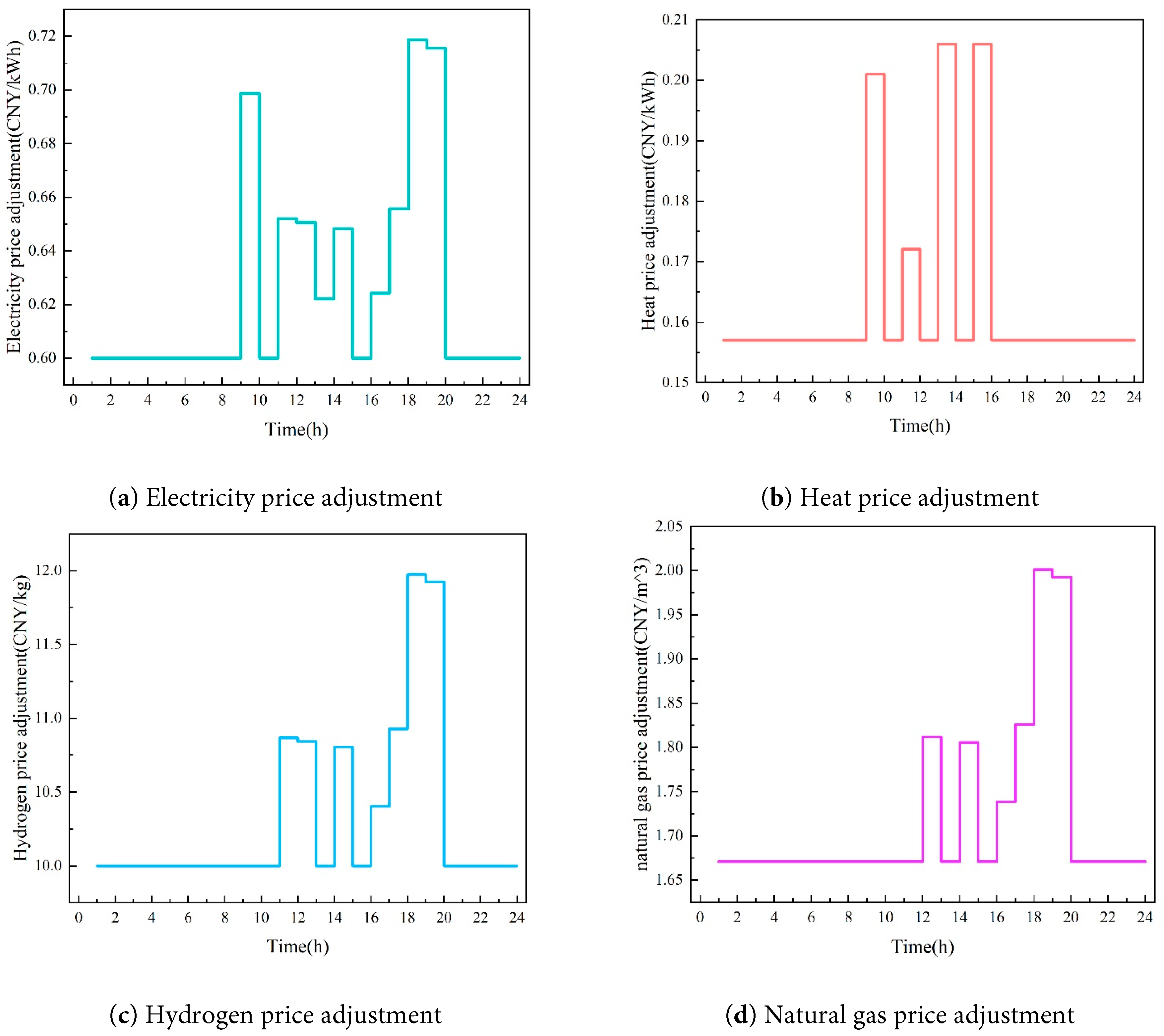
Figure 8: Dynamic price adjustment of electricity, heat, hydrogen, and natural gas.
From Fig. 8, it can be observed that the regulation prices for electricity, heat, hydrogen, and natural gas fluctuate dynamically throughout the day. The electricity regulation price peaks at 0.7186 CNY/kWh at 19:00. The heat energy adjustment price reaches its maximum of 0.2060 CNY/kWh at 13:00 and 15:00. Similarly, the regulation prices for hydrogen and natural gas both peak at 19:00, reaching 11.9765 CNY/kg and 2.0013 CNY/m3, respectively. These peaks correspond to the lower wind and solar power output on the supply side in the evening and higher electricity demand on the load side, resulting in a significant overall shortage in the EHGCS. During this time, reducing the demand for electricity, hydrogen, and natural gas plays a crucial role in alleviating the shortage and the need to purchase additional energy, which drives the regulation prices higher.
5.2.2 Analysis of the Effectiveness of Considering the Dynamic Efficiency of Electrolytic Cells and the Delayed Response of Hydrogen Fuel Cells
In the equipment output model section, this article develops a model capturing the dynamic efficiency of electrolytic cells and the delayed response characteristics of hydrogen fuel cells. To validate the model’s effectiveness, three scenarios were designed as shown in Table 6:
Table 6: Scenario setting considering the dynamic efficiency of electrolytic cells and the effectiveness of delayed response in hydrogen fuel cells.
| Scenario 1 | Scenario 2 | Scenario 3 | |
|---|---|---|---|
| Dynamic efficiency of electrolytic cell | × | √ | √ |
| Delayed response of hydrogen fuel cells | √ | × | √ |
The quantities of energy purchased and sold in the energy market under the three scenarios listed in Table 6 are shown in Fig. 9. Because the volume of natural gas traded is relatively small, the analysis focuses only on the purchased and sold electricity, heat energy, and hydrogen energy.
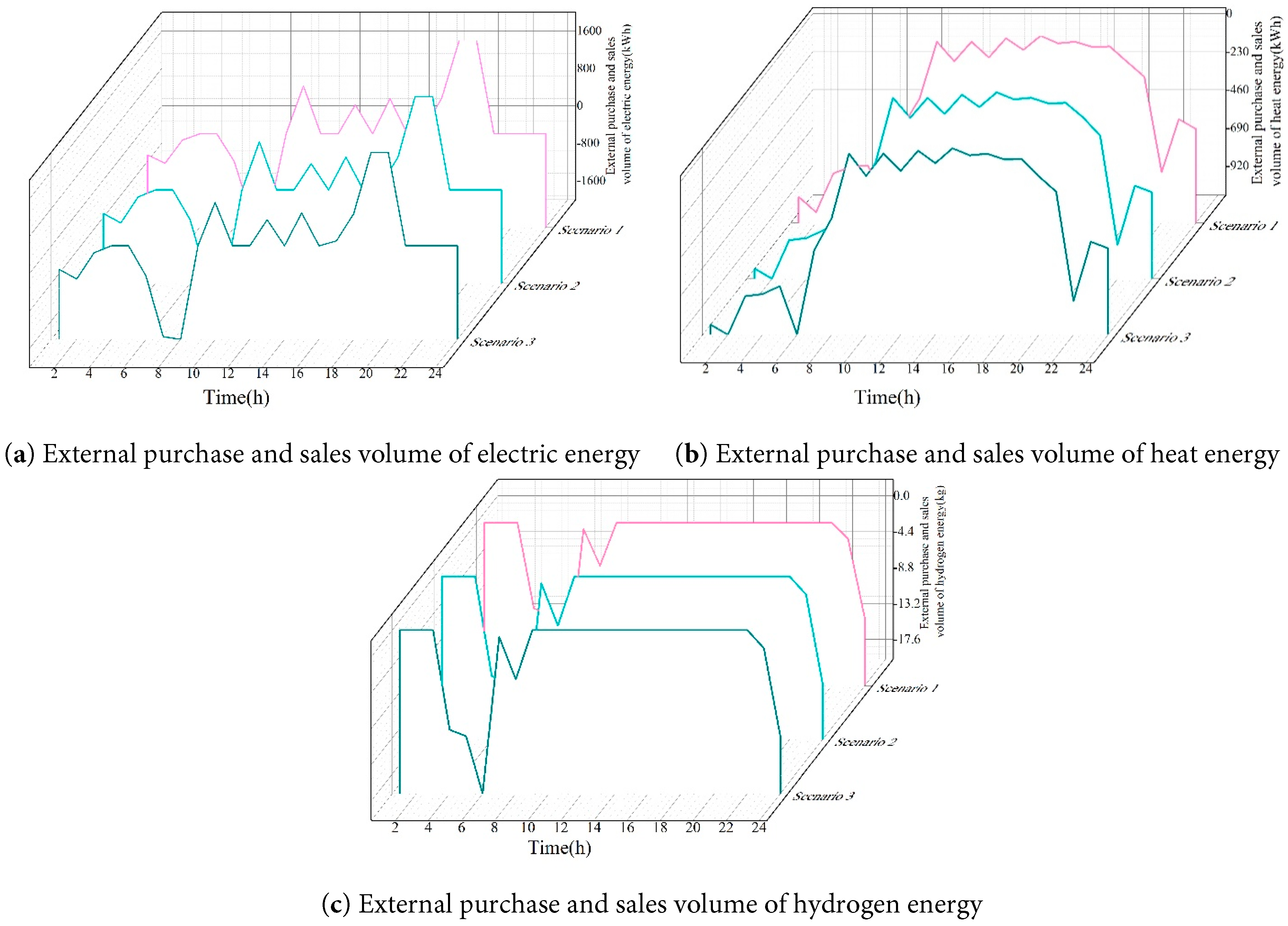
Figure 9: The amount of purchased and sold energy in the energy market under three scenarios.
As shown in Fig. 9, Scenario 1 exhibits a decrease in energy sold during the valley period from 1:00 to 8:00 compared to Scenario 3, while the purchased energy increases during 10:00, 13:00, 15:00, and 17:00–20:00. This occurs because Scenario 1 does not consider the dynamic efficiency of the electrolytic cell, causing the planned electricity consumption by the electrolytic cell to be lower than its actual consumption, which reduces market interaction during actual operation. Scenario 2 shows an increase in electricity purchased at 10:00 compared to Scenario 3, mainly due to neglecting the delayed response characteristics of hydrogen fuel cells, which decreases their actual electricity output and necessitates additional market purchases to compensate for the EHGCS shortfall.
Furthermore, the uncertainty costs and operating costs for the three scenarios are calculated and presented in Table 7:
Table 7: Uncertainty costs and operating costs in three scenarios.
| Uncertain Cost (CNY) | Uncertainty Cost Change Rate | Operating Cost (CNY) | Operating Cost Change Rate | |
|---|---|---|---|---|
| Scenario 1 | 4325.46 | 2.30% | 16,589.94 | 5.90% |
| Scenario 2 | 4384.66 | 3.70% | 15,750.24 | 0.54% |
| Scenario 3 | 4228.22 | — | 15,666.15 | — |
From Table 7, it is evident that Scenario 1, which does not consider the dynamic efficiency of the electrolytic cell, experiences increased uncertainty costs and operating costs compared to Scenario 3, with growth rates of 2.30% and 5.90%, respectively. This increase is primarily due to higher electricity purchases and reduced electricity sales, which lower EHGCS’s revenue in the energy market while raising the actual operating costs of the electrolytic cell. Scenario 2, which ignores the delayed response characteristics of hydrogen fuel cells, shows a 3.70% increase in uncertainty costs relative to Scenario 3. This is because neglecting the delayed response makes it difficult for the system to accurately predict the actual electricity output of hydrogen fuel cells, thereby increasing overall system uncertainty. These results indicate that accounting for both the dynamic efficiency of electrolytic cells and the delayed response of hydrogen fuel cells helps reduce uncertainty and operating costs in EHGCS.
In the third part of this article, a flexible adjustment capability model for multiple systems was constructed. To verify the effectiveness of this model, three scenarios were compared and evaluated. Scenario 1 did not consider the flexible regulation ability of the EHGCS. Scenario 2 only considered the flexible adjustment ability of traditional energy subsystems. Scenario 3 incorporated the flexible regulation ability of the electric-thermal-gas multiple system. The resulting imbalance of the EHGCS under these three scenarios is shown in Fig. 10.
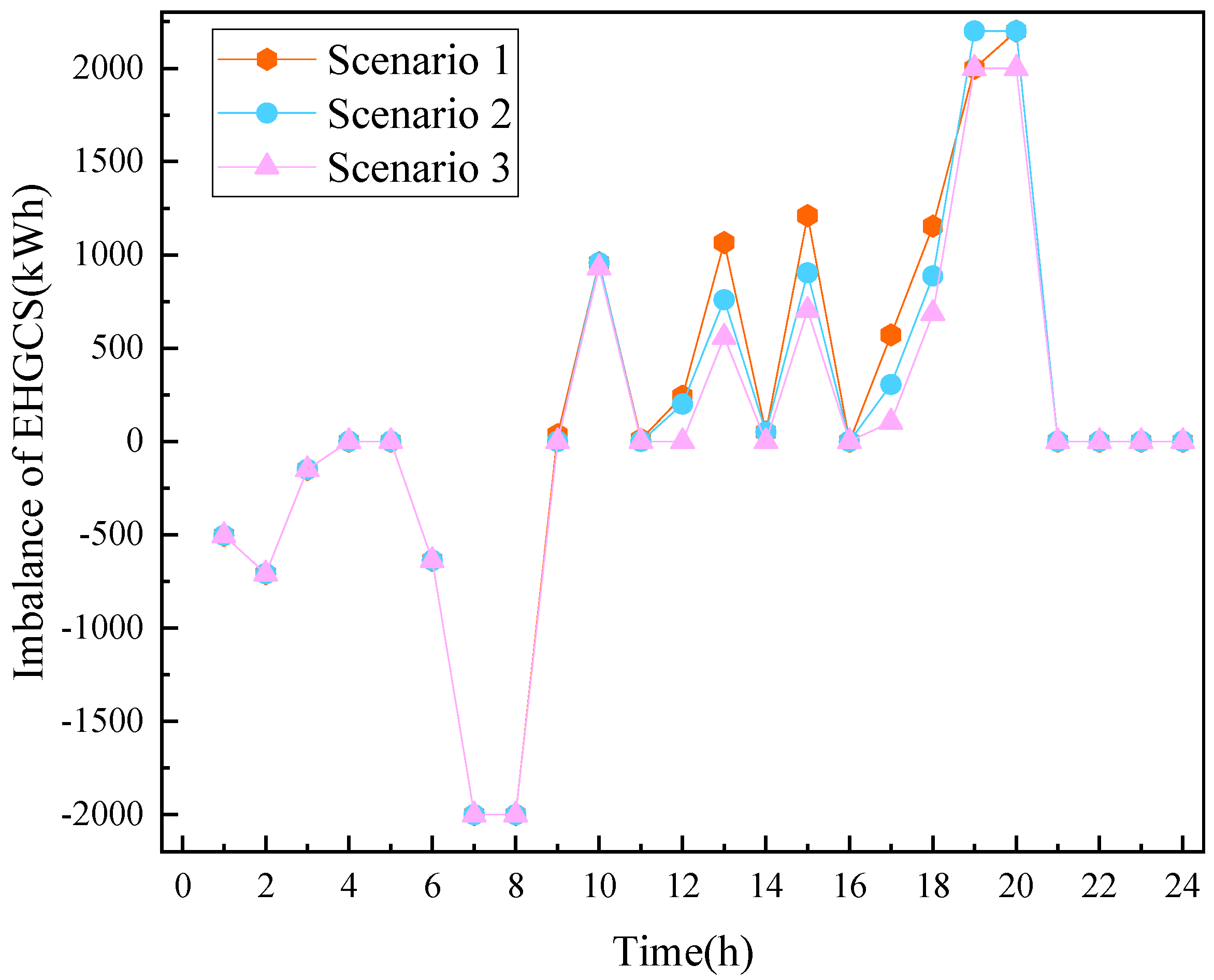
Figure 10: Imbalance of EHGCS in three scenarios.
From Fig. 10, it is apparent that Scenario 1, which does not consider regulation ability, and Scenario 2, which only considers the regulation ability of the electrical energy subsystem, exhibit significantly greater imbalance compared to Scenario 3, which accounts for the regulation abilities of multiple subsystems. The imbalance in Scenarios 1 and 2 is notably larger during peak hours from 12:00 to 18:00 than in Scenario 3. This is attributed to the insufficient utilization of adjustable capacity within EHGCS in Scenarios 1 and 2, leading to a widened supply-demand gap and increased imbalance during periods of peak energy demand. The clean energy consumption rate and user energy cost for each scenario are summarized in Table 8:
Table 8: Clean energy consumption rates in various scenarios.
| Scenario 1 | Scenario 2 | Scenario 3 | |
|---|---|---|---|
| User energy cost (CNY) | 78,236.51 | 76,268.33 | 76,066.76 |
| Clean energy consumption rate | 85.96% | 87.09% | 93.66% |
| Volume of carbon emission trading (t) | 4.88 | 4.35 | 3.57 |
| Cost of carbon emission trading (CNY) | 429.05 | 382.45 | 313.88 |
According to Table 8, compared with Scenario 3, the user energy cost in Scenario 1 and Scenario 2 increased by 2169.75 CNY and 201.57 CNY, respectively, while the clean energy consumption rate decreased by 8.22% and 7.54%. The carbon emission trading volume decreased by 1.31 t and 0.78 t, and the carbon emission trading cost decreased by 115.17 CNY and 68.57 CNY, respectively. This is mainly because Scenario 3 comprehensively considers the regulation ability of multiple subsystems, which not only reduces the energy purchase cost for users during peak hours but also provides certain compensations. Additionally, wind power output is higher during peak demand periods, when the electricity selling price in the energy market is lower. By leveraging EHGCS’s internal electricity-to-gas and gas-to-heat conversion capabilities, surplus wind power can be absorbed during peak demand periods, thus improving the clean energy consumption rate. These results indicate that considering the flexible regulation ability of the coupled electricity, heat, and gas systems can both reduce energy costs and increase the system’s clean energy consumption rate.
To further verify the effectiveness of the dynamic adjustment price model proposed in this article, the regulation capabilities of each EHGCS subsystem were compared under two pricing methods: dynamic adjustment price and fixed adjustment price, as shown in Table 9. The fixed regulation prices for electricity, heat, hydrogen, and natural gas were set at 0.65 CNY/kWh, 0.177 CNY/kWh, 11 CNY/kg, and 1.850 CNY/m3, respectively.
Table 9: The regulatory ability of each subsystem of EHGCS.
| Electricity Regulation Capacity (kWh) | Heat Regulation Capacity (kWh) | Hydrogen Regulation Capacity (kg) | Gas Regulation Capacity (m3) | |
|---|---|---|---|---|
| Fixed adjustment price | 1331.13 | 118.62 | 4.21 | 11.31 |
| Dynamically adjusting prices | 1478.70 | 128.27 | 4.74 | 12.50 |
| Growth rate of regulatory capacity | 11.09% | 8.13% | 12.49% | 10.49% |
According to Table 9, the regulation capacity of each EHGCS subsystem improved when using the dynamic price adjustment method compared to the fixed price adjustment. Specifically, the regulation capacities of electricity, heat, hydrogen, and natural gas increased by 11.09%, 8.13%, 12.49%, and 10.49%, respectively. This improvement is mainly attributed to the adjustment price being determined dynamically based on the system’s shortage and the measured contribution of regulation at each time point. Such a pricing mechanism not only reflects the real-time supply and demand conditions of EHGCS’s regulation capacity but also incentivizes users to adjust their regulation behavior rationally according to the dynamic prices, maximizing their profits and achieving a win-win outcome for both users and EHGCS.
5.2.3 Effectiveness Analysis of Considering the Correlation between Energy and Carbon Prices
This article elaborates on the correlation between the energy market and carbon market prices in the operational optimization modeling section and employs the kernel density copula method to measure the relationship between energy and carbon prices. To verify the effectiveness of this method, three scenarios were set. Scenario 1 did not consider the correlation between energy and carbon prices. Scenario 2 used the Pearson correlation coefficient to measure the correlation. Scenario 3 applied the kernel density copula method to assess the relationship between energy and carbon prices. Based on these three scenarios, the total revenue, total cost, and net revenue of the EHGCS under different conditions are shown in Fig. 11.
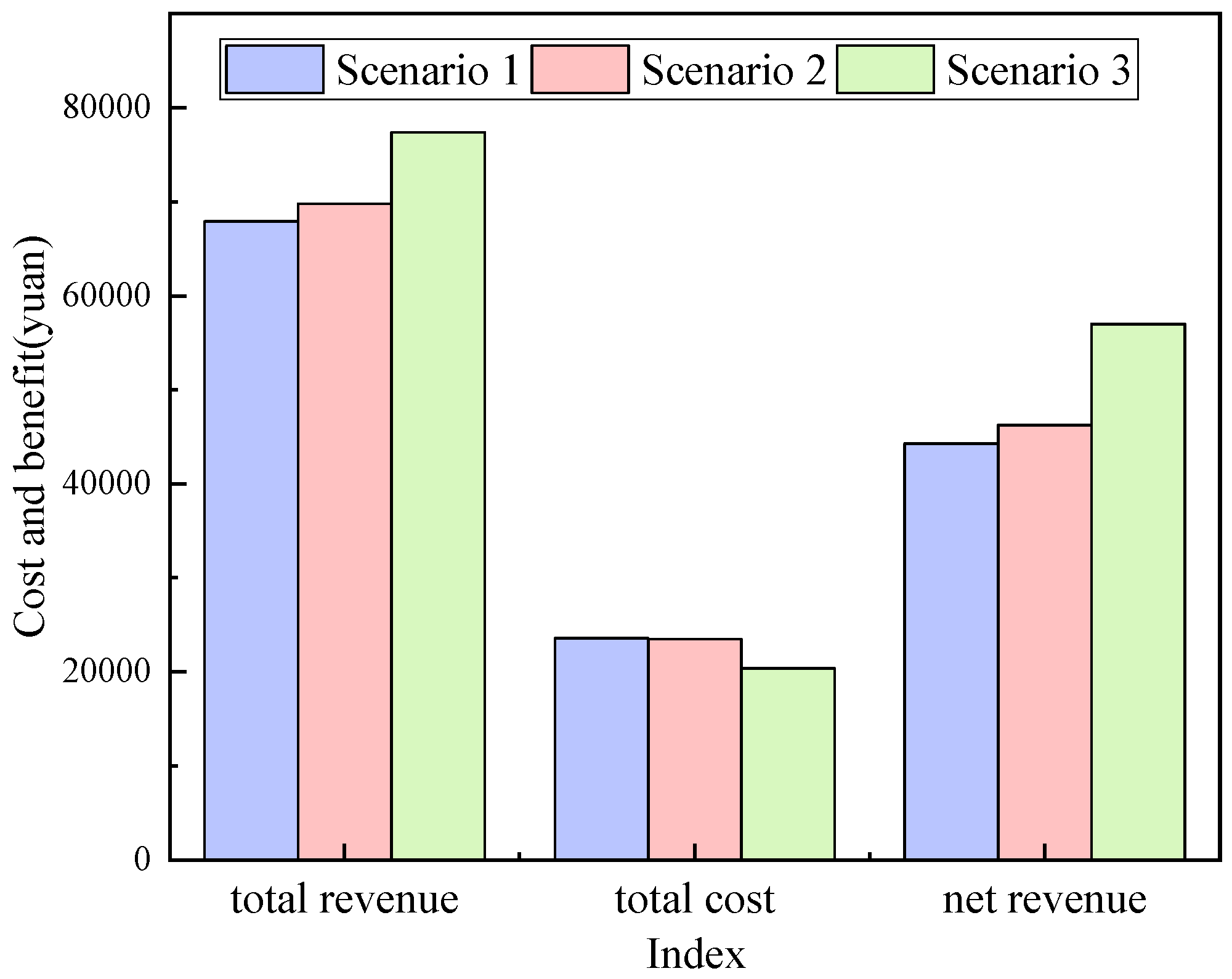
Figure 11: Cost-benefit diagram of EHGCS under different scenarios.
As shown in Fig. 11, Scenario 1 exhibits the lowest total and net returns compared to Scenarios 2 and 3. This is because Scenario 1 does not consider the price correlation between the carbon market and the energy market, resulting in EHGCS’s energy purchase and sale strategy being unable to achieve overall optimal system revenue. Specifically, when accounting for the correlation between carbon and energy market prices, EHGCS can increase gas boiler output to reduce energy market purchases when carbon prices are low, and conversely, increase purchases when carbon prices are high. Without this correlation analysis, accurate prediction of energy market price trends is not possible. Compared with Scenario 2, Scenario 3 achieves a 23.17% increase in net income. This improvement stems from the limitation of the Pearson correlation coefficient method used in Scenario 2, which only captures linear relationships, whereas market prices are influenced by multiple factors and exhibit nonlinear correlations. Thus, the kernel density Copula method applied in Scenario 3 more accurately characterizes the complex correlation between energy and carbon market prices, enhancing EHGCS’s net income.
To enhance the robustness of the results, a sensitivity analysis was performed by varying three key factors: the unit operating cost of the electrolytic cell, the unit operating cost of the carbon capture equipment, and the external market unit heat energy interaction cost. Each factor was adjusted within a range of ±20%. The impact of these variations on the net income of EHGCS is illustrated in Fig. 12.
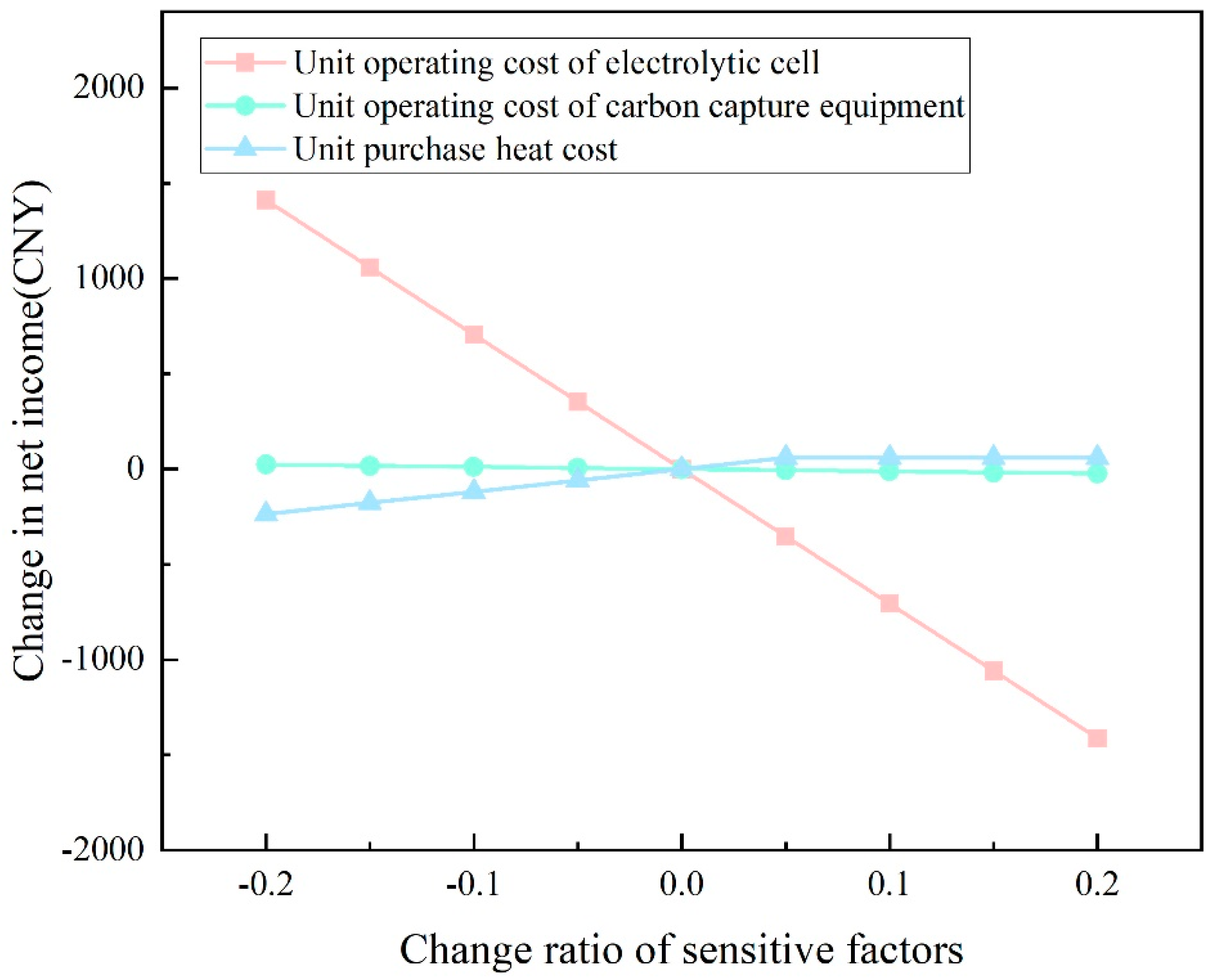
Figure 12: Results of sensitivity analysis.
As shown in Fig. 12, the unit operating costs of electrolytic cells and carbon capture equipment are negatively correlated with net income, while the external market unit heat energy interaction costs are positively correlated. Among these, the electrolytic cell operating cost has the greatest impact: a 20% decrease leads to a net income increase of 1411.47 CNY. In contrast, the carbon capture equipment’s operating cost has the least impact, with a 20% decrease raising net income by only 23.17 CNY. This difference is mainly because electrolytic cells have higher output in existing low-carbon systems, thus exerting a larger influence on system revenue.
This study proposes a novel low-carbon operational optimization strategy for an electricity-heat-gas coupling system (EHGCS), addressing limitations in previous research that often overlooked device-level dynamics, system-wide flexibility, and cross-market interactions.
First, unlike conventional models assuming static performance, this work incorporates the dynamic efficiency degradation of electrolyzers and the delayed response behavior of hydrogen fuel cells. This refined modeling enables more accurate estimation of power output and hydrogen conversion, significantly reducing external energy dependence and uncertainty-related costs.
Second, a multi-energy regulation capability model is developed, which—beyond traditional electricity and thermal regulation—integrates gas-side flexibility through electrolyzers, fuel cells, and hydrogen blending pipelines. Additionally, a dynamic pricing mechanism based on real-time regulation contribution is introduced, offering a more realistic and adaptive way to balance supply-demand and guide user participation. This dual mechanism has not been fully explored in existing literature and proves effective in improving clean energy utilization and economic efficiency.
Third, the application of a kernel density–copula method to characterize the joint behavior of energy and carbon markets is another advancement. Unlike prior studies that assume market independence or linear correlations, the proposed method enables scenario-driven decision-making under realistic market conditions. This allows the EHGCS to strategically adjust gas boiler or external electricity usage in response to carbon price variations, thus maximizing profit under emission constraints.
In summary, the integration of detailed electrochemical behavior, system-wide regulation flexibility, and price-dependent market coupling sets this study apart, offering a more accurate and adaptive framework for the low-carbon operation of future integrated energy systems.
Acknowledgement:
Funding Statement: This research received the “State Grid Jibei Electric Power Co., Ltd. Institute of Economics and Technology, Technical Innovation Costs” (SGJBJY00JJJS2400022), and we would like to express our gratitude.
Author Contributions: Conceptualization, Yan Lu, Zhongfu Tan and Jian Zhang; methodology, Yan Lu; software, Yan Lu; validation, Yan Lu, Jian Zhang and Bo Lu; formal analysis, Yan Lu; in-vestigation, Jian Zhang; resources, Jian Zhang; data curation, Jian Zhang; writing—original draft preparation, Yan Lu; writing—review and editing, Jian Zhang, Zhongfu Tan; visualization, Yan Lu; supervision, Bo Lu. All authors reviewed and approved the final version of the manuscript.
Availability of Data and Materials: The basic data used to support the findings of this study are included within the article.
Ethics Approval: Not applicable.
Conflicts of Interest: The authors declare no conflicts of interest to report regarding the present study.
Nomenclature
| Parameters | |
| the maximum output of photovoltaic power generation | |
| Charging and discharging efficiencies of the battery | |
| the depth of charge and discharge of the battery | |
| Maximum number of discharges of the battery when the discharge depth is | |
| The number of charging and discharging times when the battery device is fully charged | |
| Characteristic parameter | |
| The battery loss rate when the discharge depth is | |
| Efficiency of the hydrogen fuel cell at time t | |
| Delay response coefficient of the hydrogen fuel cell | |
| Efficiency of the electrolytic cell at time t | |
| Electric to hydrogen conversion efficiency at time t | |
| Current efficiency and voltage efficiency of the electrolytic cell at time t | |
| Power consumption per unit molar mass of hydrogen compressed by the compressor | |
| Working efficiency of the compressor. | |
| Energy charging and discharging efficiency of the hydrogen storage tank | |
| Densities of hydrogen, carbon dioxide, and natural gas, respectively | |
| Efficiency of the methanation unit. | |
| Flow rate of hydrogen and natural gas in the natural gas pipeline | |
| Calorific value of mixed hydrogen natural gas, hydrogen, and natural gas | |
| Heat generation efficiency of the electrolytic cell | |
| Heat generation efficiency of hydrogen fuel cells | |
| Efficiency of waste heat utilization | |
| Efficiency of the gas boiler | |
| Carbon dioxide emissions per unit from gas boilers | |
| Efficiency of carbon capture equipment | |
| Operating energy consumption per unit of carbon dioxide capture | |
| Fixed energy consumption of carbon capture equipment | |
| Electricity load demand during peak and normal periods at time t | |
| Peak, flat, and valley periods | |
| Maximum hydrogen production capacity of the electrolytic cell | |
| Hydrogen load demand of the user at time t | |
| Maximum transportation capacity of the pipeline | |
| Elasticity coefficient of electricity load and gas load affected by price | |
| Electricity price and gas price at time t | |
| Amount of electricity load that can be replaced before response | |
| Conversion efficiency of electricity and gas | |
| Elasticity coefficient of gas load and heat load affected by price | |
| Heat price | |
| the replaceable heat load before response | |
| Conversion efficiency of gas and heat | |
| Price of hydrogen and natural gas at time t | |
| Hydrogen purchase price and natural gas purchase price of the recipient of the gas transmission at time t | |
| Unit carbon emission rights price in the carbon market at time t | |
| Price per unit of electricity, hydrogen, natural gas, and heat energy in the energy market at time t | |
| Unit operating cost of the j-th device in the electrical energy subsystem at time t | |
| Collection of partial equipment in the electrical energy subsystem | |
| Operating cost of the s-th device in the gas energy subsystem at time t | |
| Collection of partial equipment in the gas energy subsystem | |
| Unit operating cost of gas boilers and carbon capture equipment | |
| Unit dynamic adjustment price for the w-th type of load | |
| Adjustment cost for the w-th class of load users | |
| Supply-demand deviation at time t | |
| Benchmark contribution coefficient | |
| Selling price of the w-th load in the energy market | |
| Penalty cost per unit of delayed response | |
| Purchase price of unit carbon emission rights in the carbon market at time t | |
| Purchase prices of unit electricity, hydrogen, natural gas, and thermal energy in the energy market at time t | |
| Minimum and maximum outputs of the j-th device in the electrical energy subsystem | |
| Minimum and maximum output of the s-th device in the hydrogen energy subsystem | |
| Minimum and maximum outputs of the gas boiler | |
| Minimum and maximum values of carbon capture by carbon capture equipment | |
| Minimum and maximum values of the compressor boost ratio | |
| Minimum and maximum values of electricity transmission in the energy market | |
| Minimum and maximum values of hydrogen energy transfer in the energy market | |
| Minimum and maximum values of natural gas transmission in the energy market | |
| Minimum and maximum values of heat energy transfer in the energy market | |
| Variables | |
| Output of wind power generation and photovoltaic power generation at time t | |
| Power state values of the battery at time t and time | |
| Charging and discharging power of the battery at time t | |
| Power generation and hydrogen consumption of the hydrogen fuel cell at time t | |
| Hydrogen production and power consumption of the electrolytic cell at time t | |
| Total power consumption of the compressor at time t | |
| Capacity of the hydrogen storage tank at time | |
| Energy of hydrogen storage tank charging and discharging at time t | |
| Amount of hydrogen consumed by the methanation unit | |
| Mass of carbon dioxide consumed by the methanation unit | |
| Hydrogen doping ratio at time t | |
| Residual heat generated by the electrolytic cell and hydrogen fuel cell at time t | |
| Overall utilization of waste heat at time t | |
| Heat energy generated by the gas boiler at time t | |
| Natural gas consumed by the gas boiler at time t | |
| Carbon dioxide captured by the carbon capture equipment at time t | |
| Total energy consumption of the carbon capture equipment at time t | |
| Regulation ability of the electric energy subsystem at time t | |
| Regulating ability of the thermal energy subsystem at time t | |
| Regulating ability of the gas energy subsystem at time t | |
| Substitution response of electrical load and gas load | |
| Substitution response of gas load and heat load | |
| Net income of EHGCS | |
| Total revenue and cost of EHGCS at time t | |
| Electricity, hydrogen, natural gas, and heat sold to internal users of the system at time t | |
| Hydrogen transmission rate and natural gas transmission rate of the hydrogen blending pipeline at time t | |
| Carbon emission rights sold by the system in the carbon market at time t | |
| Electricity, hydrogen, natural gas, and heat energy sold by the system in the energy market at time t | |
| Output of the j-th device in the electrical energy subsystem at time t | |
| Output of the s-th device in the gas energy subsystem at time t | |
| Adjustment amount for the w-th type of load | |
| Carbon emission rights purchased by the system in the carbon market at time t | |
| Electricity, hydrogen, natural gas, and heat energy purchased by the system in the energy market at time t | |
| Actual consumption of wind and photovoltaic power generation at time t | |
| Absorption rate of EHGCS | |
| Demand response at the time t | |
References
1. Ren K , Tang X , Huang C , Willerström J , Höök M . Prospective metal requirements assessment of China’s wind-power and photovoltaics: implications for emerging anthropogenic mines. Resour Conserv Recycl. 2025; 215: 108088. doi:10.1016/j.resconrec.2024.108088. [Google Scholar] [CrossRef]
2. Tan J , Pan W , Li Y , Hu H , Zhang C . Energy-sharing operation strategy of multi-district integrated energy systems considering carbon and renewable energy certificate trading. Appl Energy. 2023; 339: 120835. doi:10.1016/j.apenergy.2023.120835. [Google Scholar] [CrossRef]
3. National Development and Reform Commission, National Energy Administration . Implementation plan for special action on optimization of power system regulation capacity (2025–2027) [Internet]. [cited 2025 Jun 8]. Available from: https://www.gov.cn/zhengce/zhengceku/202501/content_6996643.htm. (In Chinese). [Google Scholar]
4. Tao Y , Qiu J , Lai S , Zhao J . Integrated electricity and hydrogen energy sharing in coupled energy systems. IEEE Trans Smart Grid. 2021; 12( 2): 1149– 62. doi:10.1109/TSG.2020.3023716. [Google Scholar] [CrossRef]
5. Wang Y , Wang Y , Huang Y , Yu H , Du R , Zhang F , et al. Optimal scheduling of the regional integrated energy system considering economy and environment. IEEE Trans Sustain Energy. 2019; 10( 4): 1939– 49. doi:10.1109/TSTE.2018.2876498. [Google Scholar] [CrossRef]
6. Ma Z , Witteman L , Wrubel JA , Bender G . A comprehensive modeling method for proton exchange membrane electrolyzer development. Int J Hydrogen Energy. 2021; 46( 34): 17627– 43. doi:10.1016/j.ijhydene.2021.02.170. [Google Scholar] [CrossRef]
7. Dang J , Yang F , Li Y , Deng X , Ouyang M . Transient behaviors and mathematical model of proton exchange membrane electrolyzer. J Power Sources. 2022; 542: 231757. doi:10.1016/j.jpowsour.2022.231757. [Google Scholar] [CrossRef]
8. Frensch SH , Fouda-Onana F , Serre G , Thoby D , Araya SS , Kær SK . Influence of the operation mode on PEM water electrolysis degradation. Int J Hydrogen Energy. 2019; 44( 57): 29889– 98. doi:10.1016/j.ijhydene.2019.09.169. [Google Scholar] [CrossRef]
9. Yang Y , Wu X , Ahmad M , Si F , Chen S , Liu C , et al. A direct formaldehyde fuel cell for CO2-emission free co-generation of electrical energy and valuable chemical/hydrogen. Angew Chem Int Ed. 2023; 62( 21): e202302950. doi:10.1002/anie.202302950. [Google Scholar] [CrossRef]
10. Han L , Lu PP , Wang XJ , Li MJ . Intraday optimization scheduling of power grid considering response delay characteristics of hydrogen fuel cells. Acta Energiae Solaris Sin. 2022; 43( 6): 373– 81. (In Chinese). doi:10.19912/j.0254-0096.tynxb.2022-0501. [Google Scholar] [CrossRef]
11. Dong Y , Zhang H , Ma P , Wang C , Zhou X . A hybrid robust-interval optimization approach for integrated energy systems planning under uncertainties. Energy. 2023; 274: 127267. doi:10.1016/j.energy.2023.127267. [Google Scholar] [CrossRef]
12. Pan C , Jin T , Li N , Wang G , Hou X , Gu Y . Multi-objective and two-stage optimization study of integrated energy systems considering P2G and integrated demand responses. Energy. 2023; 270: 126846. doi:10.1016/j.energy.2023.126846. [Google Scholar] [CrossRef]
13. Wang Y , Liu C , Qin Y , Wang Y , Dong H , Ma Z , et al. Synergistic planning of an integrated energy system containing hydrogen storage with the coupled use of electric-thermal energy. Int J Hydrogen Energy. 2023; 48( 40): 15154– 78. doi:10.1016/j.ijhydene.2022.12.334. [Google Scholar] [CrossRef]
14. Li P , Wang Z , Yang W , Liu H , Yin Y , Wang J , et al. Hierarchically partitioned coordinated operation of distributed integrated energy system based on a master-slave game. Energy. 2021; 214: 119006. doi:10.1016/j.energy.2020.119006. [Google Scholar] [CrossRef]
15. Wang Y , Zheng Y , Yang Q . Optimal energy management of integrated energy systems for strategic participation in competitive electricity markets. Energy. 2023; 278: 127883. doi:10.1016/j.energy.2023.127883. [Google Scholar] [CrossRef]
16. Wang Y , Zheng Y , Yang Q . Day-ahead bidding strategy of regional integrated energy systems considering multiple uncertainties in electricity markets. Appl Energy. 2023; 348: 121511. doi:10.1016/j.apenergy.2023.121511. [Google Scholar] [CrossRef]
17. Wang Q , Wang Y , Chen Z . Day-ahead economic optimization scheduling model for electricity-hydrogen collaboration market. Energy Rep. 2022; 8: 1320– 7. doi:10.1016/j.egyr.2022.08.128. [Google Scholar] [CrossRef]
18. Li J , Wang M , Wu Z , Tian G , Zhang N , Liu G . Optimal operation strategy of electricity-hydrogen regional energy system under carbon-electricity market trading. Energy Eng. 2024; 121( 3): 619– 41. doi:10.32604/ee.2023.044862. [Google Scholar] [CrossRef]
19. Tan C , Geng S , Zhao Z , Tan Z . Multi time scale operation optimization of EHHGS considering equipment uncertainty and response characteristics. J Clean Prod. 2023; 382: 135106. doi:10.1016/j.jclepro.2022.135106. [Google Scholar] [CrossRef]
20. Evers VHM , Kirkels AF , Godjevac M . Carbon footprint of hydrogen-powered inland shipping: impacts and hotspots. Renew Sustain Energy Rev. 2023; 185: 113629. doi:10.1016/j.rser.2023.113629. [Google Scholar] [CrossRef]
21. Xuan A , Shen X , Guo Q , Sun H . A conditional value-at-risk based planning model for integrated energy system with energy storage and renewables. Appl Energy. 2021; 294: 116971. doi:10.1016/j.apenergy.2021.116971. [Google Scholar] [CrossRef]
22. Kong LG , Wang SB , Cai GW , Liu C , Guo XQ . Optimization and control method for dual layer energy of zero energy building electricity hydrogen heat. Proc CSEE. 2022; 42( 17): 6196– 208. (In Chinese). doi:10.13334/j.0258-8013.pcsee.211166. [Google Scholar] [CrossRef]
23. Shao C , Feng C , Shahidehpour M , Zhou Q , Wang X , Wang X . Optimal stochastic operation of integrated electric power and renewable energy with vehicle-based hydrogen energy system. IEEE Trans Power Syst. 2021; 36( 5): 4310– 21. doi:10.1109/TPWRS.2021.3058561. [Google Scholar] [CrossRef]
24. Tan C , Tan Q , Geng S , Tan Z , Du Y , Xiao J . Multi-timescale interaction of a coupled electricity-hydrogen-gas system with a distribution network considering dynamic games. Sustain Cities Soc. 2023; 96: 104639. doi:10.1016/j.scs.2023.104639. [Google Scholar] [CrossRef]
25. Mansir IB , Bani Hani EH , Farouk N , AlArjani A , Ayed H , Nguyen DD . Comparative transient simulation of a renewable energy system with hydrogen and battery energy storage for residential applications. Int J Hydrogen Energy. 2022; 47( 62): 26198– 208. doi:10.1016/j.ijhydene.2022.02.092. [Google Scholar] [CrossRef]
Cite This Article
 Copyright © 2026 The Author(s). Published by Tech Science Press.
This work is licensed under a Creative Commons Attribution 4.0 International License , which permits unrestricted use, distribution, and reproduction in any medium, provided the original work is properly cited.
 Downloads
 Citation Tools
