Consider the Transient Stability Multi-Classification Evaluation Model for the Grid Connection of New Energy

1  Introduction

To achieve the carbon neutrality goal and meet the demands of social development, high-penetration renewable energy and power electronic devices are being increasingly integrated into traditional power systems [1]. The intermittency of renewable energy sources causes fluctuations in power generation output, necessitating frequent grid regulation to maintain power balance [2]. Meanwhile, the widespread application of power electronic devices has altered power flow distribution and significantly impaired the reactive power support capability of regional load centers [3]. As traditional synchronous generators are gradually replaced by renewable energy generation equipment, grid inertia has dropped drastically, leading to slower frequency and voltage responses as well as reduced stability following system disturbances [4]. Furthermore, as emphasized in studies on future power systems [5], the rising frequency of extreme weather events can severely disrupt renewable energy generation and grid infrastructure, further exacerbating these instability risks. These changes complicate the post-fault transient process, elevate the risk of transient instability, and pose severe challenges to the safe and stable operation of power grids. Against the backdrop of the new-type power system with high penetration of renewable energy, Virtual Power Plant (VPP) technology— which achieves the virtual integration and coordination of resources through digital technologies—has emerged as a viable solution [6,7]. By combining real-time measurement data (e.g., bus voltages, branch powers, power angle differences) with fast transient stability assessment algorithms, the VPP control system can conduct real-time monitoring of transient instability risks. Upon identifying a risk, the results of transient stability analysis directly trigger emergency control strategies—such as rapidly adjusting distributed generation output, shedding non-critical controllable loads, and switching energy storage operation modes. These measures suppress the propagation of transient disturbances within a time frame from milliseconds to seconds, thereby preventing system instability. However, the network structure of modern power systems has grown increasingly complex, and the widespread adoption of power electronic devices has significantly increased the feature dimensionality of measurement data. Moreover, under scenarios with high renewable energy penetration, the dual uncertainties on both the generation and load sides not only result in highly variable operating conditions of power systems but also intensify the complexity of feature coupling among physical variables. Conventional binary classification models are no longer adequate to meet the stringent safety requirements of modern new-type power systems. Therefore, developing a multi-class transient stability assessment algorithm integrated with renewable energy grid connection has become an urgent and critical issue to be addressed.

The effective application of deep learning to this task faces two primary and interconnected challenges: extraction and characterization of complex spatiotemporal features of power system, and the inherent class imbalance in training samples [8]. The first challenge originates from the nature of the measurement data itself. The widespread deployment of wide-area measurement systems (WAMS) provides substantial data support for data-driven intelligent assessment models. When a power system undergoes large-scale disturbances or faults, it is typically accompanied by abrupt changes in electrical quantities such as—bus voltage phasors and line transmission power—resulting in post-fault response trajectories that exhibit complex time-varying characteristics. To analyze the dynamic behavior of power systems, researchers have therefore adopted models proficient in processing temporal data, including Long Short-Term Memory (LSTM) networks [9], Temporal Convolutional Networks (TCN) [10,11], and Gated Recurrent Units (GRU) [12,13]. However, these studies primarily focus on mining temporal correlations within power big data, often neglecting the spatial structural information inherent in data features. To enhance the comprehensiveness of feature extraction from power system data, a hybrid method combining TCN and Graph Convolutional Networks (GCN) was proposed in [11]. This approach uses TCN to extract temporal features between electrical quantities and employs an adaptive GCN to mine spatial dependencies and inter-dimensional relationships among features. This design enables the model to maintain high performance and strong generalization capability even in scenarios involving changes to grid topology. Nevertheless, this model exhibits two key limitations: it is highly dependent on the accuracy and completeness of grid topology data, and it incurs substantial computational costs. In [9], LSTM is utilized to capture temporal characteristics, while the Relief-F algorithm is applied to select features with greater spatial relevance based on inter-sample differences. A critical drawback of this method, however, is the high sensitivity of the Relief-F algorithm to sample randomness, which can lead to instability in feature selection results. The study in [12] introduced an enhanced convolutional residual memory network based on GRU, which utilizes GRU for temporal feature extraction and residual modules for spatial feature extraction. Still, the relatively simple architecture of GRU limits its performance when handling high-dimensional power data in renewable-rich scenarios. Building on these insights, our proposed TCN-IResNeXt hybrid model is specifically designed to address the unique requirements of transient stability assessment. Compared to GCN-based models and other deep learning approaches (e.g., traditional CNNs, shallow neural networks), our improved ResNeXt module—integrated with a Triplet Attention mechanism—directly captures intricate spatial correlations from data channels. This eliminates reliance on pre-defined graph topologies, endowing the model with greater adaptability and robustness, particularly in scenarios involving uncertain or dynamically changing grid structures. In contrast, the TCN backbone outperforms LSTM/GRU models in two key aspects: it achieves superior computational efficiency through parallel processing, and by leveraging dilated causal convolutions and residual blocks, it excels at capturing long-term temporal dependencies while ensuring gradient stability. The performance of data-driven transient stability assessment (TSA) models depends on both effective feature representation and balanced training datasets. However, owing to the stringent reliability and security requirements of power systems, real-world instances of post-fault instability are extremely rare—primarily because stability control and relay protection systems promptly intervene to prevent such scenarios. This scarcity of unstable scenarios leads to severe class imbalance in training datasets [14].

The second challenge emanates from the operational realities of power systems. Regarding the intrinsic class imbalance problem, it arises from the fact that severely unstable scenarios are scarce in practical power grid operations relative to stable and mildly unstable scenarios. In current research, solutions to the class imbalance problem are primarily addressed through two types of approaches: data-level and algorithm-level methods. At the data level, common techniques include sampling-based methods, generative model-based methods, and instance-based transfer learning. Sampling-based methods mitigate class imbalance by either augmenting minority-class samples or reducing majority-class samples, with typical strategies including under sampling [15] and oversampling [16,17]. Generative model-based methods learn underlying data distributions to synthesize new samples and are widely employed in data augmentation. Popular generative models include generative adversarial networks (GANs) and their variants [18], diffusion probabilistic models [19], and variational autoencoders (VAEs) [20]. However, although synthetic samples generated by these methods follow the minority-class distribution, they often fail to fully capture the nuances of real-world power system operating conditions, such as dynamic load fluctuations or renewable energy output variability—limiting their practical utility for stability assessment. Instance-based transfer learning utilizes domain-specific knowledge from a source domain to improve model performance in a target domain [21], which can effectively alleviate data scarcity in the target domain. Nevertheless, these approaches depend on the critical assumption that sample distributions in the source and target domains are similar. With the growing integration of renewable energy, power system fault scenarios have become increasingly complex—featuring more frequent voltage dips and multi-mode oscillations—leading to significant distribution drift between domains and elevating the risk of negative transfer. At the algorithm level, widely adopted strategies encompass model ensemble [22,23] and cost-sensitive learning [24,25]. Ensemble methods combine predictions from multiple classifiers to reduce individual model bias and improve generalization to unseen fault scenarios, whereas cost-sensitive learning adjusts decision thresholds by assigning higher misclassification costs to the minority class samples—prioritizing the accurate detection of critical instability events. A key limitation of these approaches, however, is their narrow focus on binary-classification-based TSA. They have not been adequately extended to finer-grained multi-class stability scenarios. However, these approaches typically focus solely on binary-classification-based transient stability assessment and have not been sufficiently extended to finer-grained multi-class stability scenarios.

To address the aforementioned challenges, this paper proposes a novel TSA model for power systems with high renewable energy penetration integration. The main contributions are summarized as follows:

1.    To enhance the model’s feature extraction capability, a spatio-temporal feature fusion network termed TCN–IResNeXt is proposed. This network integrates Temporal Convolutional Network (TCN) with an improved ResNeXt (IResNeXt) augmented by attention mechanisms, aiming to simultaneously capture temporal dependencies and spatial structural information from high-dimensional power system data. A Triplet Attention module is embedded into the ResNeXt architecture, which operates on the high-dimensional tensor generated after feature extraction and captures inter-channel spatial correlations through a triple-branch structure. Finally, a gated fusion unit is employed to integrate temporal and spatial features, thereby enhancing the model’s ability to extract and discriminative comprehensive features.

2.    To address the significant class imbalance issue in power system stability classification, an enhanced loss function scheme based on the entropy of posterior probabilities is proposed. The selected boundary samples are then augmented through data augmentation techniques, and a boundary-aware loss term is incorporated to refine the original loss function. The improved loss function mitigates the model’s bias induced by imbalanced data distribution, significantly enhances its capability to recognize boundary samples, and ultimately boosts the overall classification performance of the model.

2  Multiscale Feature Extraction Network Combing TCN and IResNeXt

When a power system is subjected to large-scale disturbances, the outcome of stability assessment is jointly determined by the spatial correlations among key system variables and their temporal evolution characteristics. Consequently, the feature extraction network must be capable of not only mining the dynamic evolution patterns of electrical features over time, but also capturing the nonlinear spatial coupling features among different electrical parameters—a task that conventional deep learning models often struggle to accomplish through an integrated approach.

To address these challenges, this paper proposes a new TCN–IResNeXt network—a spatio-temporal architecture whose innovation resides in the multi-scale, layer-wise integration of its dual branches through gating modules. These gates orchestrate the fine-grained fusion of temporal and spatial features across network layers, ensuring the two types of features are intricately combined throughout the learning process. This approach enables comprehensive modeling of power system dynamics, thereby facilitating enhanced feature representation for transient stability assessment. As illustrated in Fig. 1, the model adopts a parallel data processing paradigm: a TCN branch captures multi-scale temporal dependencies via dilated convolutions, while an IResNeXt branch extracts high-dimensional spatial features using its cardinality structure. The gating mechanism continuously fuses these features across scales, with the final outputs concatenated and fed into the classification module. This synergistic design ensures the model develops a cohesive understanding that spans from local details to global correlations.

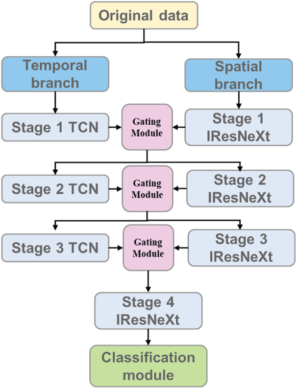
Figure 1: Schematic of the TCN–IResNeXt architecture

2.1 Temporal Feature Extraction at Multiple Scales Using TCN

TCN is a deep learning model specifically designed for time series processing. It adopts a unique causal convolutional architecture, ensuring that the output at the current time step depends solely on the current and past inputs, thereby preserving the temporal order of the sequence [26]. The structural composition of the TCN is illustrated in Fig. 2. For a one-dimensional input time series, the operation of a dilated causal convolution layer can be mathematically formulated as Eq. (1):

H(t)=∑s=0S−1w(s)⋅xt−d⋅s(1)

where, H(t) denotes the output feature at time step t, w(s) represents the s-th weight of the convolutional kernel, xt−d⋅s refers to the input value at time t − d⋅s, d denotes the dilation factor, and S denotes the size of the convolution kernel. After the dilated causal convolution operation, features extracted from different network layers are subsequently integrated via residual connections to mitigate the vanishing gradient problem and enhance feature propagation.

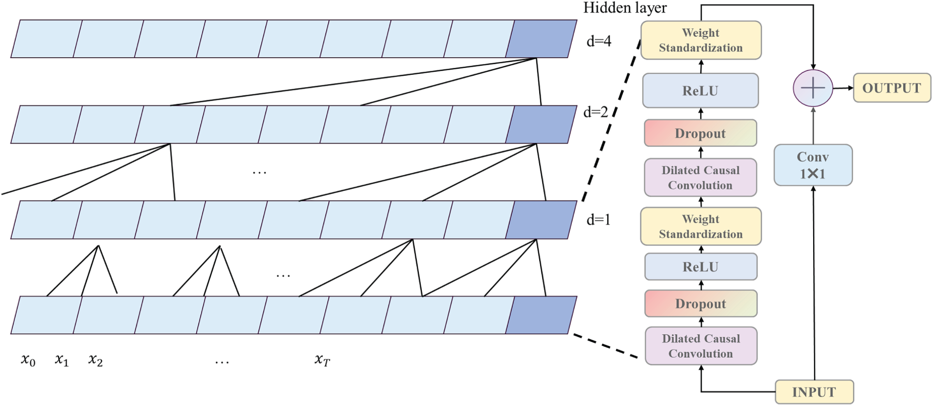
Figure 2: TCN network structure

Given that the evolution of power system transient processes adheres to swing equations with time as the independent variable, the TCN constructs multi-scale temporal receptive fields through the combined effect of varying dilation factors and convolution kernel sizes. Specifically, a base receptive field with d = 1 captures short-term temporal dependencies, an expanded receptive field with d = 2 extracts medium-term temporal relationships, and a large receptive field with d = 4 captures long-term evolutionary patterns. In this paper, features from convolutional layers with different receptive fields are hierarchically integrated, enabling comprehensive extraction of multi-scale temporal characteristics from power system data.

2.2 Multi-Dimensional Spatial Feature Extraction Based on Improved ResNeXt

While the TCN model exhibits remarkable effectiveness in capturing temporal features and time-varying correlations among sensitive electrical quantities during fault transient intervals, modeling the complex spatial coupling relationships among these parameters remains equally essential for transient stability assessment of power systems.

ResNeXt is a deep residual network that enhances spatial feature extraction by stacking multiple residual blocks, enabling feature representation from local to global scales [27]. However, since all convolutional kernels in the original ResNeXt share the same weights, the model lacks adaptability to enhance or suppress spatial features across different regions. To address this limitation, we introduce a Triplet Attention module into the residual structure of ResNeXt. This module uses a triple-branch architecture to capture interactions among channel-wise, temporal, and spatial dimensions of the input tensor, thereby dynamically recalibrating channel weights through attention mechanisms [28]. The structure of the proposed improved ResNeXt network is shown in Fig. 3.

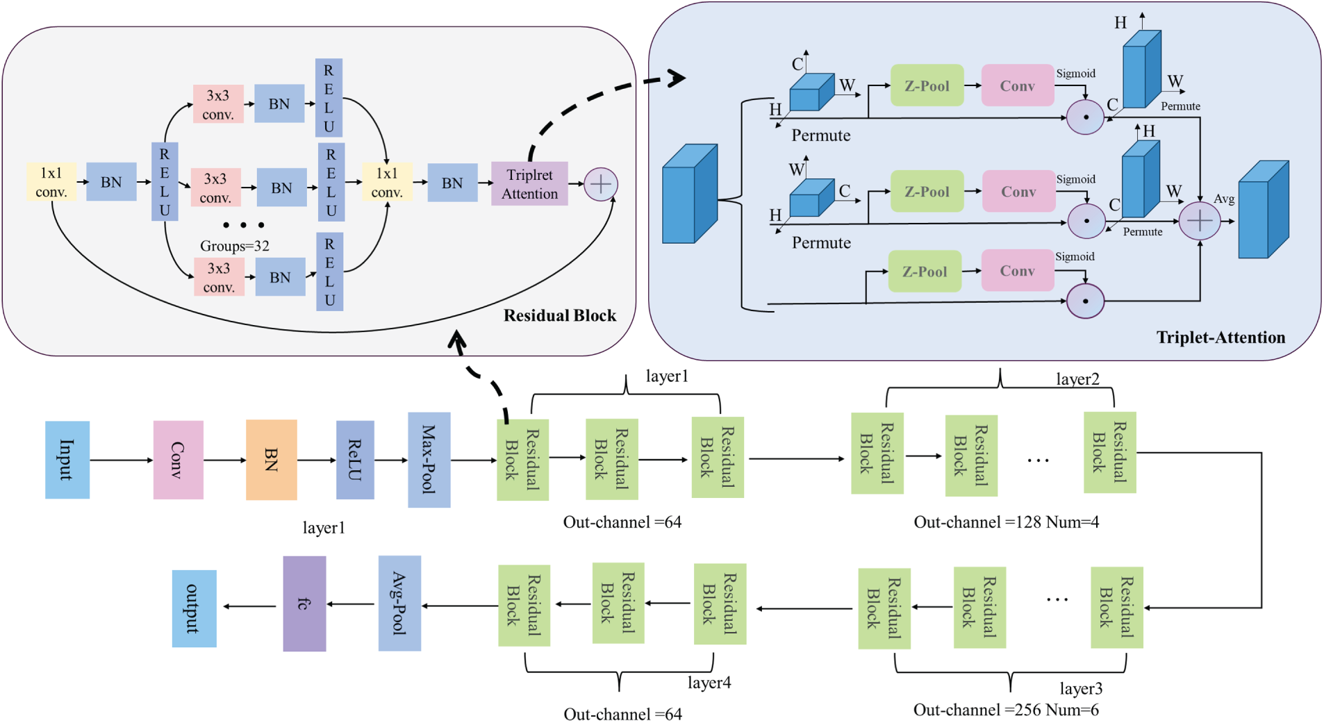
Figure 3: Improved ResNeXt network structure

As shown in Fig. 3, each residual block adopts a grouped convolution design, which reduces the number of parameters while enhancing the model’s expressive capacity. An identity mapping mechanism is incorporated to ensure stable gradient propagation throughout the network. The hierarchical feature transformation within the residual network can be expressed by Eq. (2):

XL=X0+∑i=0L−1Fi(Xi,Wi)(2)

where, XL denotes the output features of the current stage, L represents the number of residual blocks in an arbitrary stage, X0 refers to the input feature to the stage, and Xi and Wi correspond to the input features and weights of the i-th residual unit, respectively. Fi denotes the nonlinear transformation within the residual block.

The chain rule of gradients for the residual blocks is given by Eq. (3):

∂E∂Xl=∂E∂XL(1+∂∂Xl∑i=lL−1Fi(Xi,Wi))(3)

where E denotes the loss function and ∂E∂XL represents the gradient of the final output of the current stage. This formulation ensures that the identity mapping term ∂E∂XL has at least one propagation path without attenuation, thereby effectively mitigating the gradient explosion problem.

In this paper, a Triplet Attention module is integrated into the residual block to enhance the network’s ability to capture critical information through dynamic feature weight reassignment. The specific implementation is illustrated in the top-right subfigure of Fig. 3: For an input tensor denoted as x ∈ R(C × H × W), the Triplet Attention module first performs dimension permutation to form three branches, each computing attention weights in a differently oriented tensor space.

In the first branch, x is transposed to form x1 ∈ R(W × H × C), which is then processed through a pooling layer and a standard convolutional layer. The pooling layer consists of two parallel paths—max pooling and average pooling—that perform down-sampling on x1. The outputs of these two paths are concatenated and passed into a standard convolutional layer to generate spatial attention. This convolutional layer is composed of a 2D convolution (Conv2d), batch normalization (BN), and a ReLU activation, with a kernel size of 7. Finally, a sigmoid activation is applied to produce the attention weight ω1 of this branch. The second branch transposes x into x2 ∈ R(H × C × W) and repeats the same procedure to obtain attention weight ω2. The third branch operates directly on the original input x without transposition, similarly producing an attention weight denoted ω3. The output tensor Y, enhanced by attention, is obtained by multiplying the input tensor of each branch with its corresponding attention weight, followed by average aggregation. This process can be expressed by Eq. (4):

Y=13(x1ω1¯+x2ω2¯+xω3)(4)

where (∙)¯ denotes the transpose operation.

2.3 Multi-Scale Spatio-Temporal Feature Extraction Network Based on TCN-IResNeXt

This paper proposes combining TCN with IResNeXt to construct a multi-scale spatiotemporal feature extraction network. Through hierarchical feature interaction, this network achieves synergistic perception of data, enabling the fusion of temporal and spatial features from power-related data across multiple scales. The structure of the proposed feature extraction network is illustrated in Fig. 4.

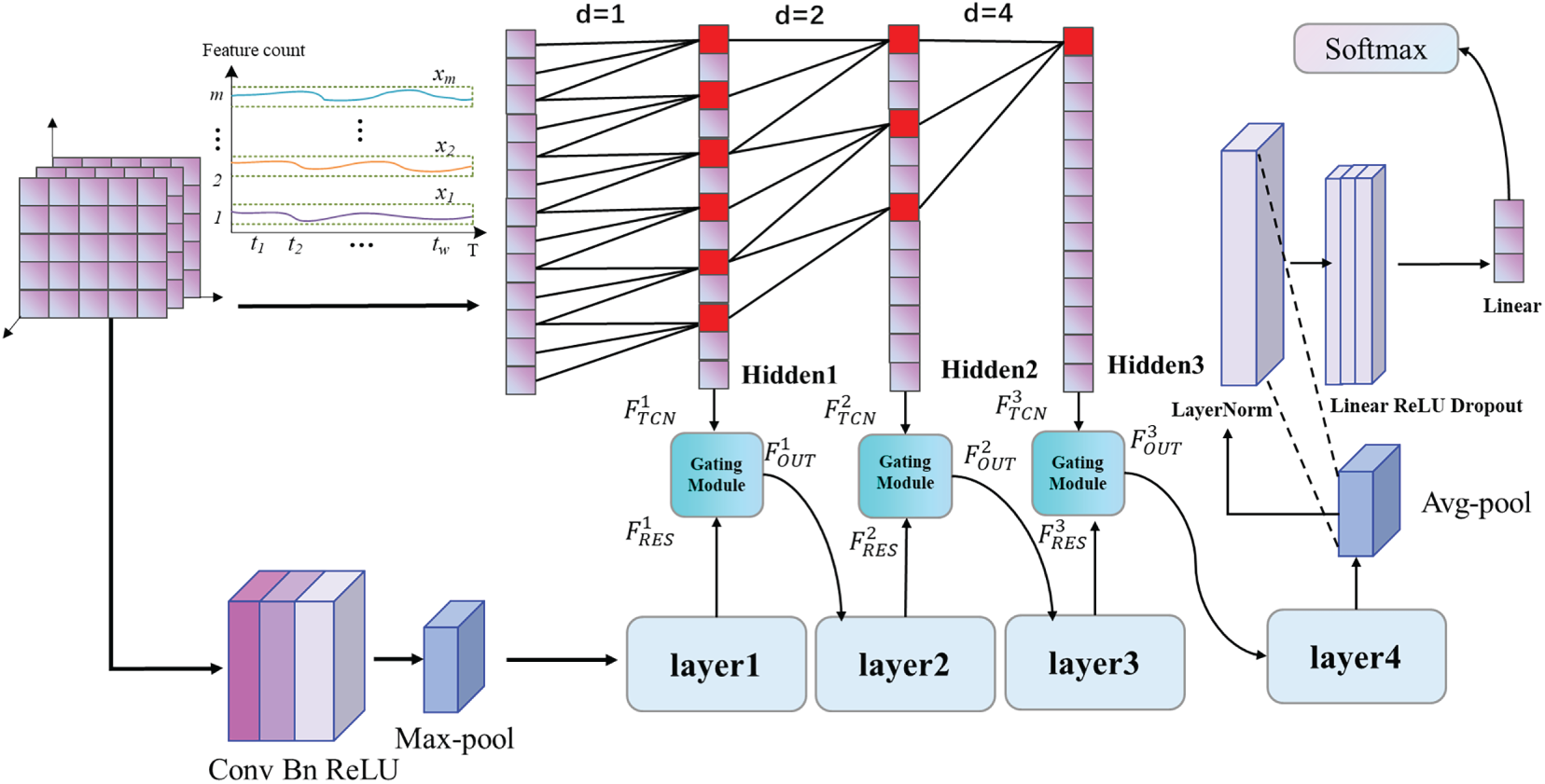
Figure 4: TCN-IResNeXt feature extraction network

The multi-scale feature extraction process is carried out as follows: Sampled data are fed into the feature extraction network. The TCN branch performs multi-scale temporal analysis through causal convolutional layers with exponentially increasing dilation rates. The IResNeXt branch consists of four sequentially connected residual block groups, which progressively expand the receptive field to construct structural relational representations. The outputs from each hidden layer of the TCN branch, denoted as FTCNi (i∈(1,2,3)), are extracted and fused with the outputs from the first three residual block groups of the IResNeXt branch, denoted as FRESi (i∈(1,2,3)).

To achieve effective fusion of the outputs from the TCN and IResNeXt branches, a gating unit is introduced as illustrated in Fig. 5. To ensure dimensional consistency, each FTCNi is first upsampled via interpolation to match the spatial size and dimensionality of the corresponding FRESi, followed by a 1 × 1 convolution for feature alignment and concatenation. The aligned features are then processed through another 1 × 1 convolution and a Softmax activation function for normalization to generate a spatially-aware weight distribution. The weight calculation is expressed by Eq. (5):

G=Softmax(Wgatei∗[FRESi||FTCNi])(5)

where Wgatei denotes the gating convolutional weights, initialized using the Kaiming method.

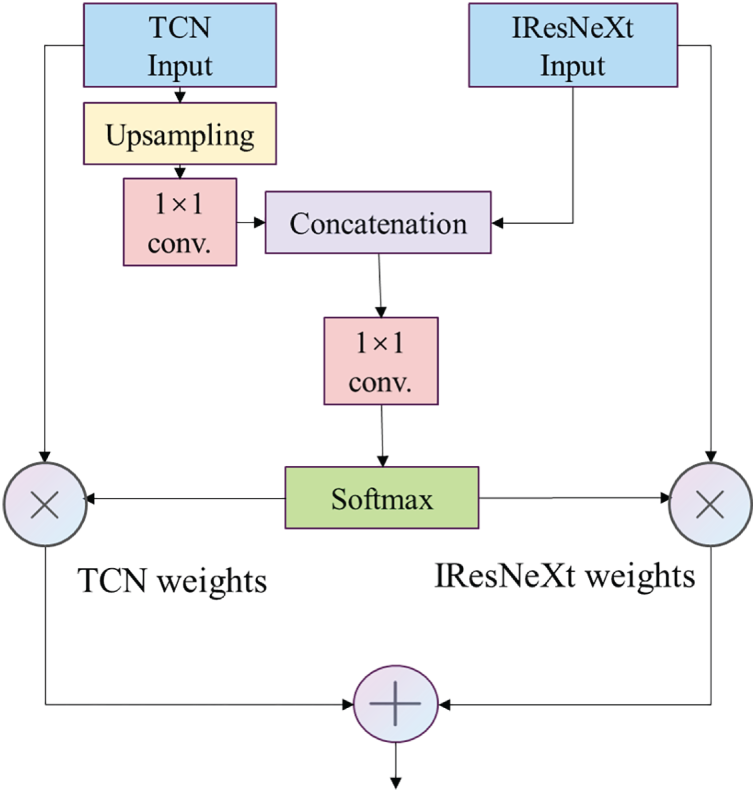
Figure 5: Gated fusion unit

The fused feature FOUTi is obtained by adaptively weighting the spatial and temporal features using G, and then passing the result to the next stage of the IResNeXt network. This process can be formulated as:

FOUTi=G0⊙FRESi+G1⊙FTCNi(6)

where G0 and G1 represent the weight vectors assigned to the IResNeXt branch and the TCN branch, respectively.

This fusion mechanism offers two key advantages. Firstly, it comprehensively captures both the inherent temporal dependence and spatial correlation in the power data, enabling multi-scale feature extraction from local to global levels. Secondly, it enhances the discriminative ability of spatiotemporal features, improves the model’s sensitivity to critical patterns, and facilitates effective multi-scale integration. Consequently, the fused features preserve the complete spatial structure of the original data while seamlessly incorporating temporal dynamics, thereby achieving joint spatiotemporal optimization across multiple network levels.

3  A Multi-Stage TSA Based on the Dual-Tower Transformer

Modern power systems possess high robustness, often enabling automatic recovery to a stable state following disturbances. Consequently, stable samples dominate the dataset, leading to a pronounced class imbalance problem. In transient stability classification tasks, model gradients are predominantly influenced by samples of the majority class (stable cases). This imbalance tends to obscure the decision boundary and compromise the model’s accuracy in identifying critical samples near the classification boundary—samples that typically belong to the minority class (unstable cases). To address this issue, an improved loss function is introduced to refine the decision boundary, encouraging the model to focus more on minority class samples. Consequently, the recognition and representation of critically unstable instances are significantly enhanced.

3.1 Feature Set Construction

When the system is subjected to disturbances such as three-phase short-circuit faults or transmission line outages, the rotor angles of synchronous generators undergo large-scale oscillations. If a rotor angle exceeds its critical threshold during the first swing, the system loses synchronism due to energy imbalance, resulting in first-swing instability. If the stability limit is breached after several oscillations, multi-swing instability occurs. Conversely, if the oscillation amplitude of the rotor angle gradually decays and converges to an equilibrium value, the system returns to a stable state. The power angle curves corresponding to these three scenarios are illustrated in Fig. 6.

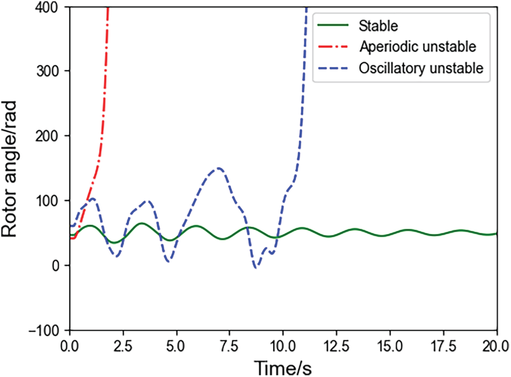
Figure 6: Curve of power angle variation

In the context of renewable energy integration, multi-swing instability occurs with increasing frequency. During voltage dips triggered by large-scale disturbances, grid-forming converters inject reactive current to support voltage and maintain connectivity. Following fault clearance, these converters gradually restore active power output and suppress power angle oscillations. If the post-fault power angle does not exceed the critical value, or the system damping is sufficient to dissipate oscillation energy, the power angle will return to equilibrium in 1–2 cycles, and the system remains transiently stable. Otherwise, if repeated voltage drops trigger multiple mode transitions, or if the coordination between converters and synchronous generators is inadequate, the rotor angle may undergo multi-cycle oscillations. This process eventually leads to the disconnection of renewable energy clusters and causes multi-swing instability [29]. Given that different instability modes are governed by distinct mechanisms and require specific control measures (e.g., mitigating first-swing instability relies on faster fault clearance, whereas addressing multi-swing instability requires enhanced damping), it is essential to distinguish between these two instability modes and implement appropriate preventive and control strategies. This ensures the security and stability of the power system.

3.2 Loss Function Improvement Considering Boundary Samples

During the training of the multi-class assessment model, the posterior probability distribution of the samples contains rich information about the classification process. The posterior probability distribution of an input sample over all classes, derived via the Softmax function, reflects the model’s confidence in its prediction. In addition to this, it also implicitly encodes the class imbalance present in the training data and the distribution characteristics of the samples in the feature space. Building on this insight, an improved loss function scheme that leverages posterior probability distribution is proposed. The specific implementation steps are as follows:

1.    Calculation of Posterior Probability Distribution: The posterior probability distribution of an input sample is given by Eq. (7):

P(y=c|z)=ez(k)∑k=13ez(k),k∈{1,2,3}(7)

where z=[z1,z2,z3] denotes the outputs of the fully-connected layer, c=[0,1,2] represents the sample labels, and k is the index of the target class.

2.    Entropy and Boundary Sample Identification: The uncertainty of the probability distribution can be quantified by its entropy. The sample entropy H(z), computed from the posterior probabilities, is defined by Eq. (8):

H(z)=−∑c=02P(y=c|z)log⁡P(y=c|z)(8)

Samples with high entropy values in their posterior probability distributions are identified as critical boundary samples requiring heightened model attention. These typically correspond to instability cases involving oscillatory instability leading to power grid disconnection. The identification of boundary samples is achieved by comparing the entropy value against a dynamically updated threshold τ, which follows a linear decay learning schedule:

τ(t)=max(0.1,τ(0)−η⋅t)(9)

where τ(0) is the initial threshold value, η is the decay rate, empirically set to 0.01, and t denotes the current training iteration. A sample is identified as a boundary sample if its entropy H(z) exceeds the threshold τ. For the transient stability assessment model proposed in this paper, a sensitivity analysis of the initial threshold τ(0) performed within the range (0.1, 0.5). The optimal value of τ(0) is determined based on the model’s evaluation performance, and the relationship between τ(0) and the model’s accuracy is illustrated in Fig. 7.

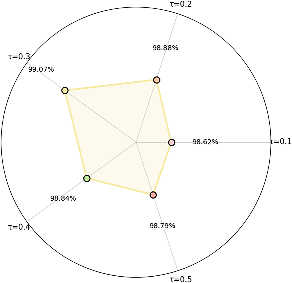
Figure 7: Impact of τ on Accuracy of the modle

Experimental results indicate that the proposed assessment model achieves the highest classification accuracy (99.07%) when the initial threshold τ(0) is set to 0.3. Therefore, τ(0) is fixed at 0.3 in all subsequent simulation analyses.

3.   Boundary Sample Augmentation and Loss Function Improvement: In the conventional cross-entropy loss, the weighting scheme assumes a uniform distribution across all classes, which often results in the misclassification of samples near ambiguous decision boundaries. To address this issue, we propose an enhanced loss function that incorporates the entropy of the posterior probability distribution. The improved loss function is defined as follows:

Loss=1N∑i=1Nwi⋅CE(zi,yi)(10)

CE(z,y)=−∑k=13y(k)⋅log⁡(exp⁡(z(k))∑k=13exp⁡(z(k)))(11)

wi={α1if H (zi)>τotherwise}(12)

As can be seen from Fig. 8, the model achieves the optimal classification performance when the initial value of α is set to 2.0. The linear decay mechanism of α can effectively adjust the weight of augmented data in the overall optimization objective, thereby enhancing the learning of boundary features in the early stage of training and ensuring stable convergence in the later stage, which avoids overfitting to the augmented samples.

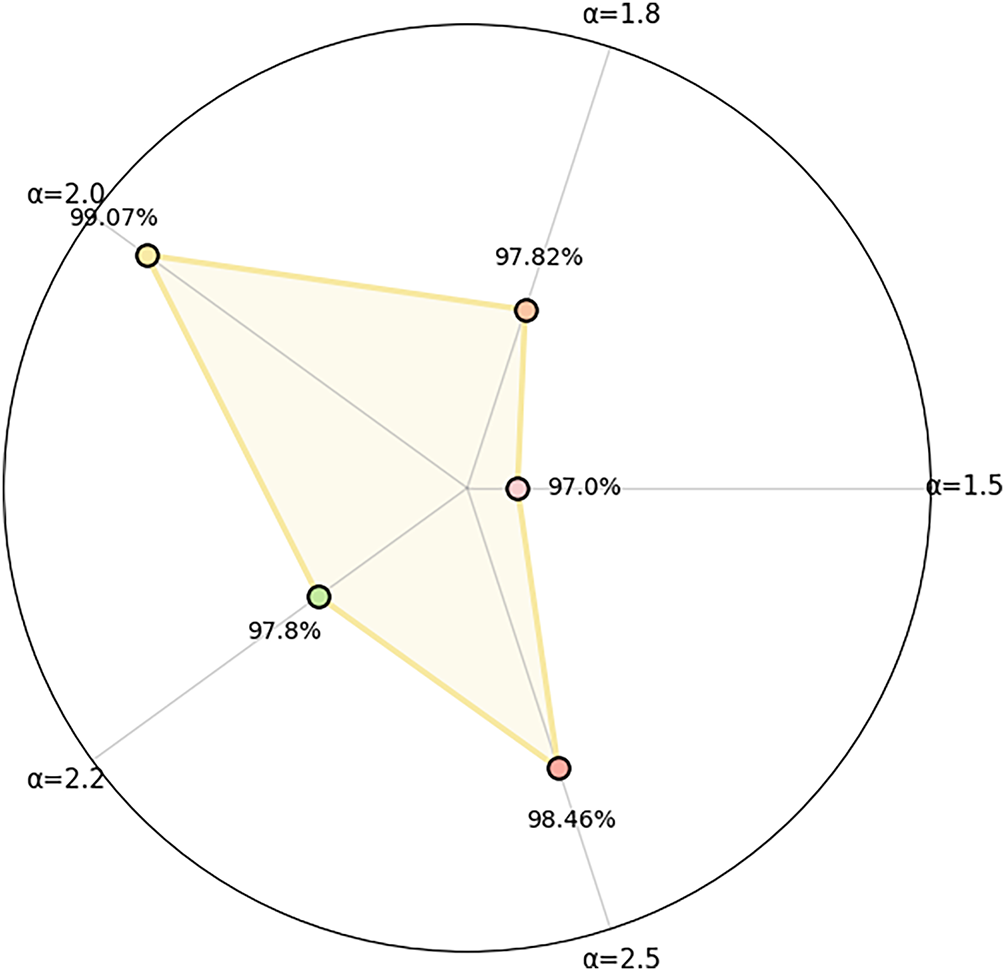
Figure 8: Impact of α on Accuracy of the modle

The loss function is adaptively adjusted via wi: when boundary samples are detected, dynamic data augmentation (by adding noise) is applied specifically to these samples within each training batch. The augmented cross-entropy loss Laug is recalculated using Eq. (11), which greater emphasis placed on boundary samples at high risk of misclassification. The total loss Ltotal for the evaluation model is given by Eq. (13):

Ltotal=N⋅Loss+αM⋅LaugN+αM(13)

where M denotes the number of boundary samples.

4  Transient Stability Assessment

4.1 Dataset Construction

For the transient stability assessment task, the construction of a high-quality dataset follows these fundamental principles: first, selecting electrical parameters that are strongly correlated with the mechanism of transient stability analysis; second, ensuring that these parameters are readily obtainable directly from phasor measurement units (PMUs).

In the mechanistic analysis of direct methods for system stability assessment, the transient energy function is closely related to the system’s stability status [30]. When the dissipation term is ignored, the energy function consists of a network term Vnet, a generator term Egen, and a load term Eload, as expressed in Eq. (14):

W=Vnet+Egen+Eload(14)

where Vnet relates to nodal voltage magnitudes and phase angles, and can be written as:

Vnet=−12∑BiiVi2−∑i<jBijViVjcos⁡θij(15)

here, Bij represents the admittance, V the voltage magnitude, and θij the phase angle difference. Meanwhile, Egen and Eload are functions of voltage magnitudes, phase angles, and the active and reactive power of generators and loads, as given in Eq. (16):

Egen+Eload=−∑gen(∫Pgidθi+Qgidln⁡Vi)+∑load(∫PLidθi+QLidln⁡Vi)(16)

From Eqs. (15) and (16), it is evident that electrical quantities such as bus voltage magnitudes, phase angles, and generator active/reactive power are highly correlated with the system’s transient stability level and directly reflect its energy balance state. Therefore, this paper selects these key electrical quantities to construct the assessment dataset. The sampling period covers three critical stages: pre-fault steady-state operation, fault occurrence, and the dynamic process after fault clearance.

The stability label of each sample is determined based on the Transient Stability Index (TSI), which is derived from the generator rotor power angles after fault clearance, as defined in Eq. (17):

TSI=(360∘−|Δδmax|)/(360∘+|Δδmax|)(17)

where Δδmax denotes the maximum power angle difference between any two generators relative to the reference generator. A sample is classified as transiently stable if the maximum relative rotor angle difference among all generators remains below 360° and the power angle difference curve exhibits an oscillatory and decaying trend. Otherwise, it is considered transiently unstable. Furthermore, for unstable samples, first-swing instability and multi-swing instability are distinguished based on the oscillation damping ratio of the power angle difference, as proposed in [31].

4.2 Assessment Framework

To effectively enhance the classification performance of the model and reduce the probability of missed detections of instability, this paper proposes a multi-stage transient stability assessment method. The framework consists of three phases: dataset generation, model training, and online assessment, as illustrated in Fig. 9.

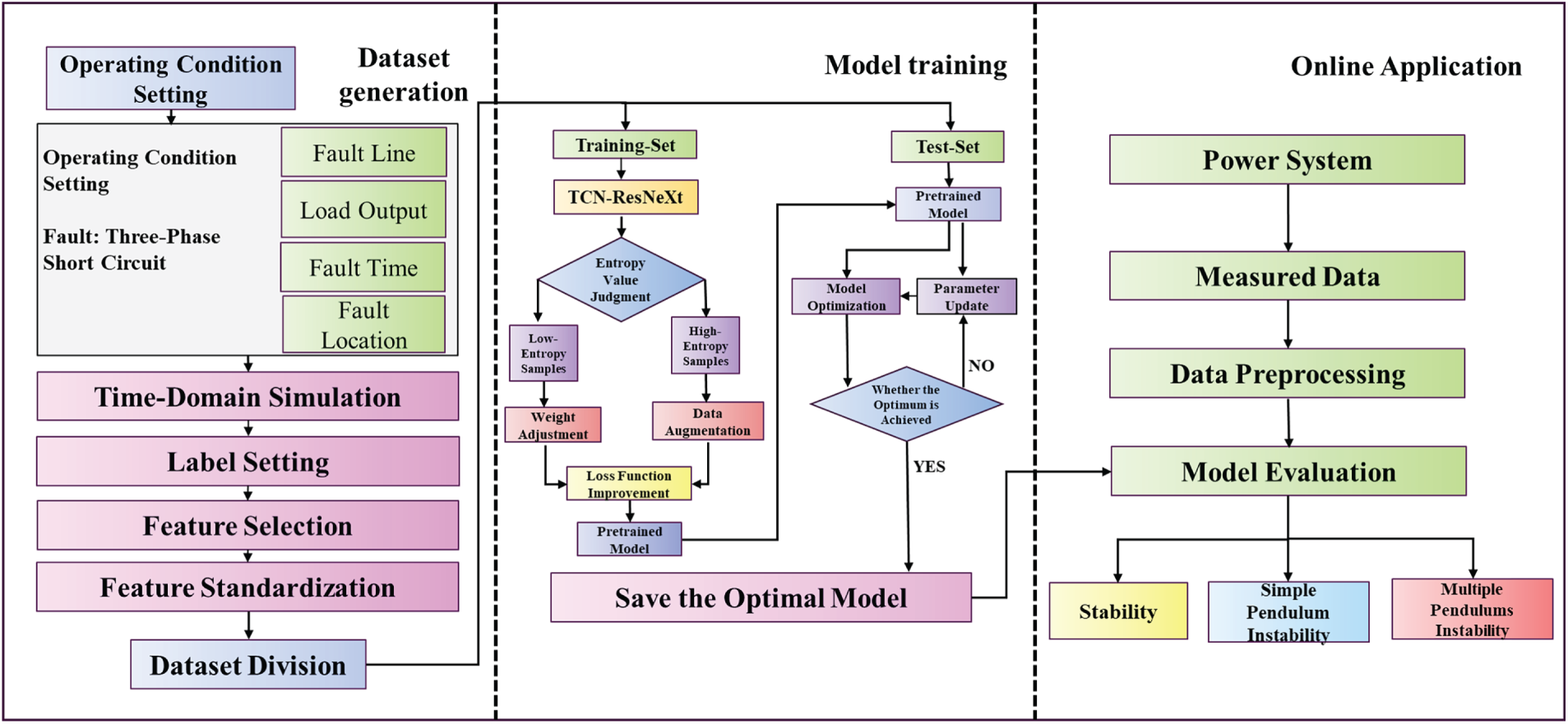
Figure 9: Transient stability assessment flowchart

Various operating conditions are configured by adjusting load levels, fault locations, fault lines, and fault durations. Time-domain simulations are performed to generate sample data. The fault type is set to the severe three-phase short-circuit fault. System load levels are set to 80%, 85%, …, 120%, totaling nine levels. Faults are applied to lines connected to each busbar, at locations of 0%, 20%, 40%, 60%, and 80% along the line. The fault duration is randomly set within the range of 0.1–0.2 s, and the total simulation time is 20 s. After labeling the samples using the TSI criterion, the data are normalized via Eq. (18):

Z=a−μσ(18)

where Z is the normalized value, a is the input data, μ is the mean, and σ is the standard deviation. The generated dataset is split into training and testing sets in an 8:2 ratio.

The model is initially trained on a large-scale dataset. The TCN-IResNeXt feature extraction network, with its hierarchical architecture, captures multi-scale temporal and spatial features, enabling comprehensive characterization of the data. To further optimize performance, a modified cross-entropy loss function is employed as the cost function. By augmenting high-entropy samples and introducing a boundary loss term, the model’s sensitivity to boundary samples is enhanced. The NAdam optimization algorithm is adopted to dynamically update model parameters. Finally, the pre-trained model is fine-tuned on the training set, and the multi-class assessment model is derived using the parameters yielding optimal accuracy.

During the online assessment phase, real-time grid data are sampled and evaluated by the trained model, which computes the probability values P0, P1, and P2 corresponding to the stable, first-swing unstable, and multi-swing unstable classes, respectively. The sample is classified as stable if P0 exceeds both P1 and P2; as first-swing unstable if P1 is the highest; and as multi-swing unstable if P2 dominates the probability output.

5  Case Analysis

5.1 Data Set and Assessment Indicators

The simulations were implemented in Python using the PyTorch deep learning framework. Experiments were conducted on two test systems: the CSEE-DAS system and the IEEE 140-bus system. Three-phase short-circuit faults were applied with parameters configured as described in Section 4.2. In the CSEE-DAS dataset, the distribution among the three classes was approximately 6.8:2.2:1, corresponding to 5878 stable, 1901 first-swing unstable, and 864 multi-swing unstable samples. In the IEEE 140-bus system, the distribution among the three classes was approximately 7.9:0.5:1, corresponding to 18,434 stable, 2458 first-swing unstable, and 1229 multi-swing un-stable samples. This distribution aligns with the expected statistical characteristics of the N-1 security criterion, which requires power systems to generally remain stable under single-element contingencies.

The CSEE-DAS system has a total installed capacity of 4.8 GW from renewable sources and 6.0 GW from conventional generation. This configuration reflects a high penetration level of renewable energy, rendering it particularly suitable for studying “double-high” power grids with high power electronics penetration. Single-line diagrams of both test systems are provided in Appendix Fig. A1.

To comprehensively evaluate model performance, multi-class evaluation metrics are defined as shown in Eqs. (19)–(22):

PACC=T00+T11+T22T0+T1+T2×100%(19)

F1i=2×TiiT0i+T1i+T2i×TiiTi0+Ti1+Ti2TiiT0i+T1i+T2i+TiiTi0+Ti1+Ti2(20)

Recalli=TiiTi0+Ti1+Ti2(21)

Gmean=(Recall0×Recall1×Recall2)1/3(22)

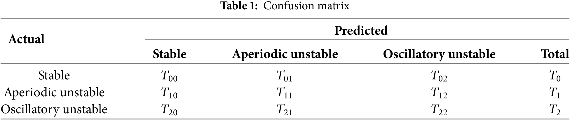
where Tij denotes the number of samples whose true class is i and predicted class is j, as defined in the confusion matrix (Table 1). PACC represents the overall accuracy, reflecting the model’s general classification performance. F1i is the harmonic mean of precision and recall: precision indicates the reliability of the model, while recall measures its ability to identify positive samples. The metric Recall denotes the true positive rate, and Gmean is the geometric mean of recall values across all classes. Both F1 and Gmean are crucial metrics for evaluating classification performance under imbalanced sample distributions.

5.2 Comparison of Assessment Performance among Different Models

To validate the superiority of the proposed TCN-IResNeXt hybrid architecture in power system transient stability assessment, a rigorous comparative experimental scheme was designed. Five representative benchmark models were selected as controls: a standard TCN model, a ResNeXt model, an LSTM model [32], a Transformer model [33], and an XGBoost-DF model [22]. The model parameters were configured as follows: In the TCN-IResNeXt model, the TCN branch employs a 3-layer dilated causal convolution with dilation factors [1, 2, 4]; the ResNeXt branch adopts a 4-layer residual structure with a cardinality of 32. The standalone TCN model maintains the same structure as the TCN branch within our proposed model. The standalone ResNeXt model uses the standard ResNeXt-50 configuration. The LSTM model has 4 hidden layers with 256 units each. The Transformer model uses 8 attention heads and 4 encoder sub-layers.

All deep learning models were optimized using the Nadam optimizer and trained for 200 epochs with a batch size of 128. The initial learning rate was set to 0.0002, which was reduced upon observing no improvement in validation loss for five consecutive epochs. The results is the average of 20 experiments. The evaluation performance of each model on the CSEE-DAS system is shown in Table 2.

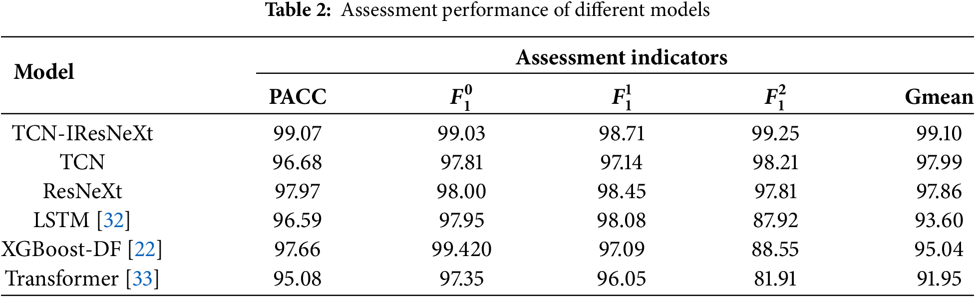
Experimental results demonstrate that the proposed model achieves improvement across all performance metrics for transient stability assessment compared to conventional deep learning models. This enhancement is primarily attributed to the designed dual-branch feature extraction architecture: the temporal modeling branch effectively captures multi-scale temporal dependencies through dilated causal convolutions, while the spatial modeling branch, with its grouped convolution structure, extracts deep nonlinear spatial correlations among key parameters such as voltage and power angle. The integration of temporal and spatial information is further enhanced by a gated fusion unit, enabling dynamic and complementary feature interaction. Notably, the model shows improved performance in identifying minority classes such as multi-swing instability, with the F12 score increasing by 1.04% compared to the best baseline model. These results validate the practical applicability and robustness of the proposed fusion model in complex power system scenarios.

To further verify the generalizability of the proposed model in conventional power systems, additional simulations were conducted on the IEEE 140-bus system. The results are summarized in Table 3.

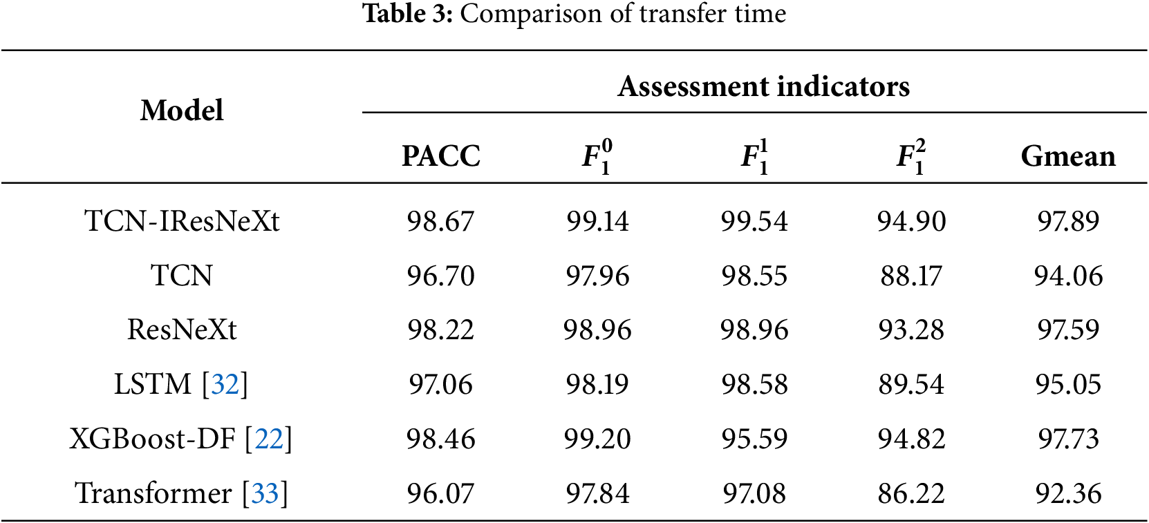
As shown in the table, the proposed model maintains high classification accuracy even in this large-scale traditional system, outperforming all other benchmark models. Furthermore, significant improvements are observed across all evaluation metrics, particularly for minority-class samples. These results demonstrate the strong adaptability and generalization capability of the proposed model across different grid configurations.

5.3 Clustering Visualization of Sample Features

To validate the effectiveness of the hierarchical feature extraction in the proposed dual-branch network, the output features FOUTi from each layer were visualized using t-SNE for dimensionality reduction. The results are shown in Fig. 10.

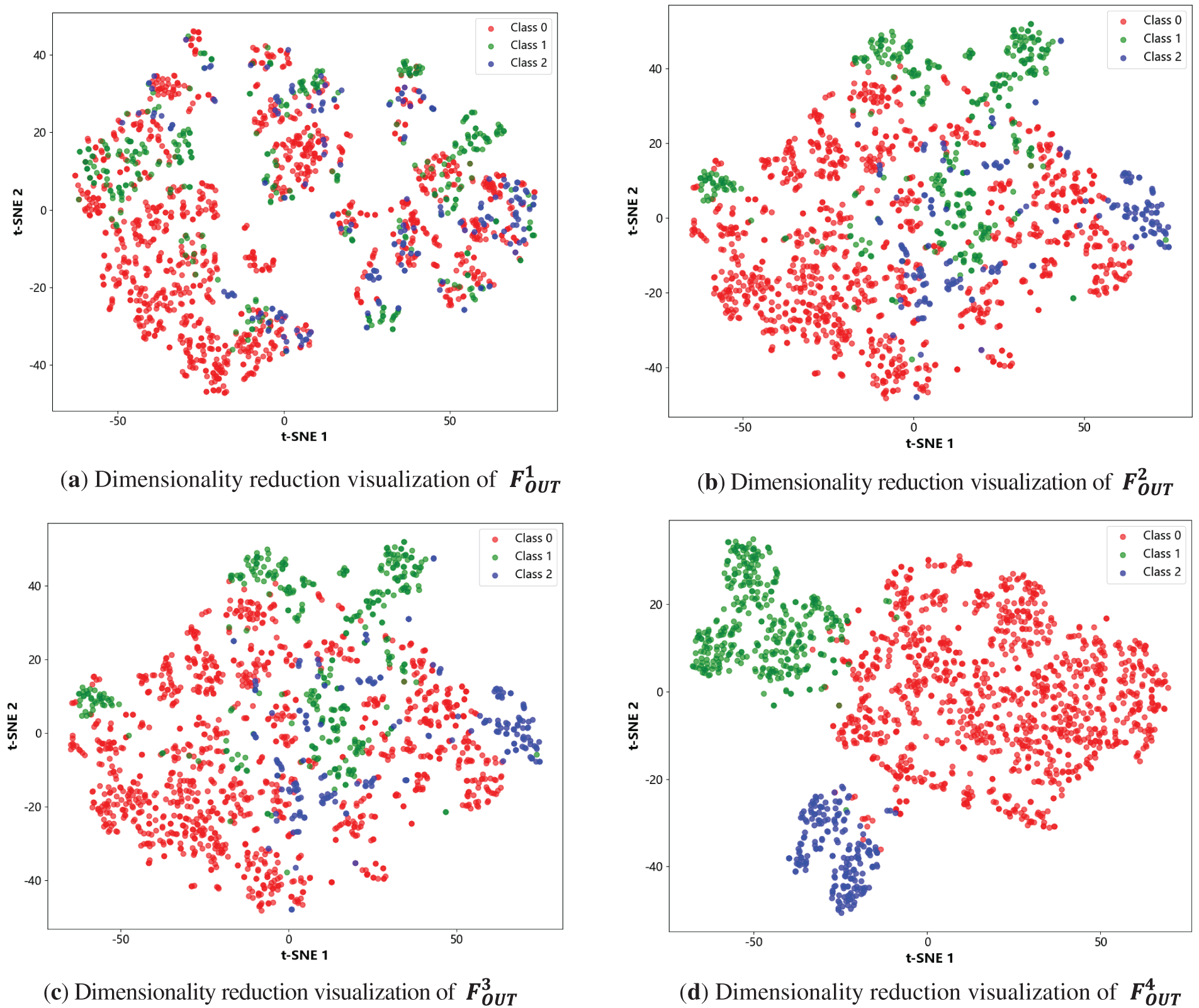
Figure 10: Dimensionality reduction visualization

As depicted in Fig. 10, the t-SNE visualizations of features from Layer 1 to Layer 4 demonstrate a clear evolution in clustering performance. As the network depth increases, the clustering effect becomes increasingly distinct: samples belonging to the same class gradually aggregate into more compact and separable groups. In the first layer, features from different classes are heavily intermixed. While the second and third layers begin to form preliminary cluster structures, significant overlap persists near decision boundaries. By the fourth layer, the features form well-separated, spherical clusters with minimal inter-class confusion. This result demonstrates that the model’s classification performance improves progressively with each layer, and the multi-scale fusion architecture effectively captures feature representations from local patterns to global contexts.

5.4 Comparative Analysis of the Impact of Loss Functions on Classification Performance

To validate the superiority of the proposed improved loss function over conventional loss functions, a comparative analysis was conducted using confusion matrices derived from different loss functions. The loss functions compared include cross-entropy loss, L1 loss, and binary cross-entropy loss. Simulations were performed on the CSEE-DAS system, with the experimental results presented in Fig. 11.

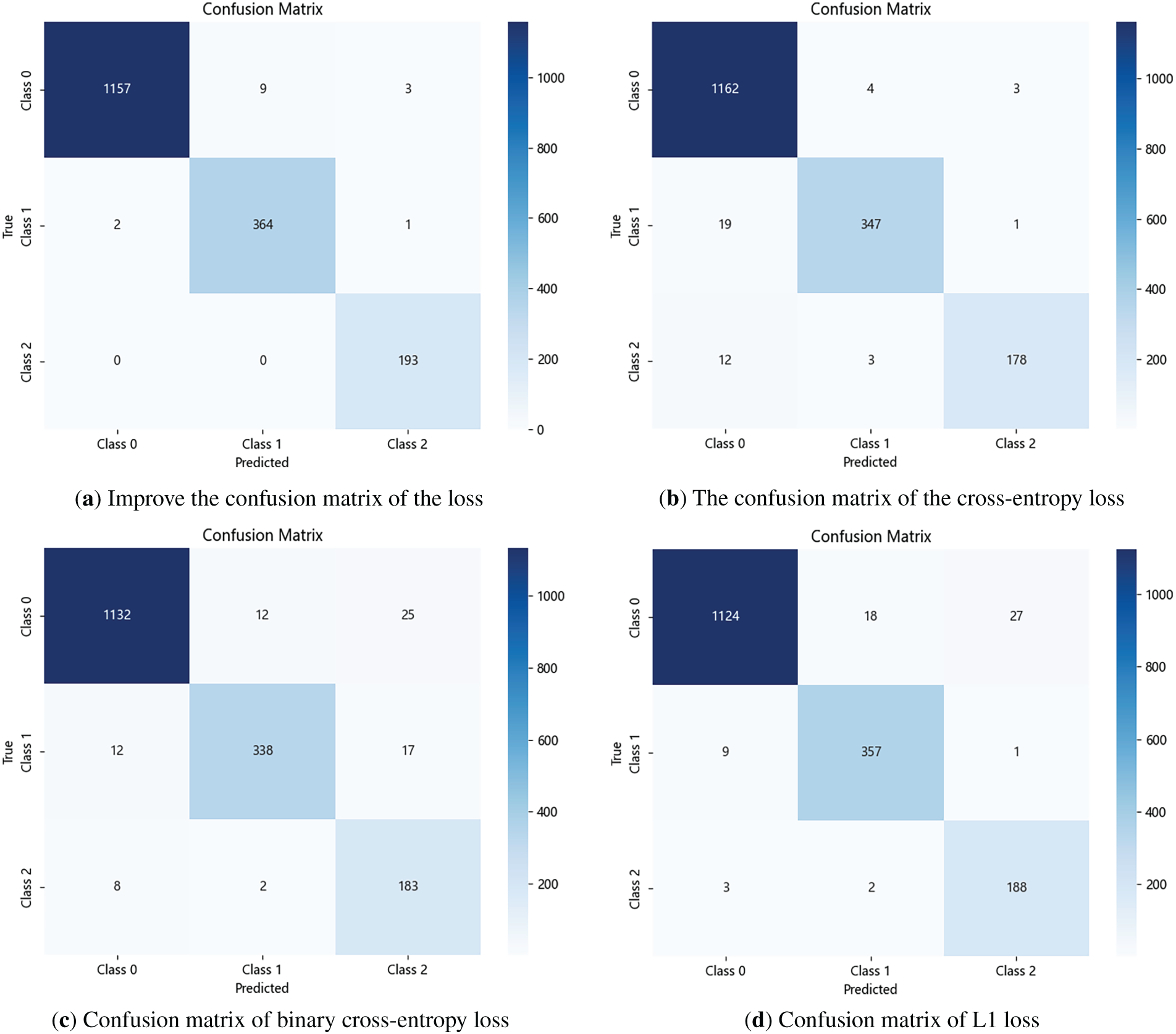
Figure 11: Confusion matrix

By examining the number of misclassified samples in the confusion matrices, it is evident that the model trained with the proposed loss function exhibits superior performance in reducing misclassification errors.

The Kappa coefficient (K) is a statistical metric used to evaluate the consistency and reliability of classification models, particularly in scenarios with class imbalance. It is defined as follows:

K=P−Pe1−Pe(23)

where P represents the overall classification accuracy, and Pe denotes the sum of the expected values along the diagonal of the confusion matrix. Let T be the total number of samples in the confusion matrix, Tm,: the total number of samples in the m-th row, and T:,m the total number of samples in the m-th column.

The expected agreement Pe is computed as:

Pe=∑m=03(Tm,:×T:,m)(T)2(24)

A comparison of the Kappa coefficient values across different loss functions is shown in Fig. 12.

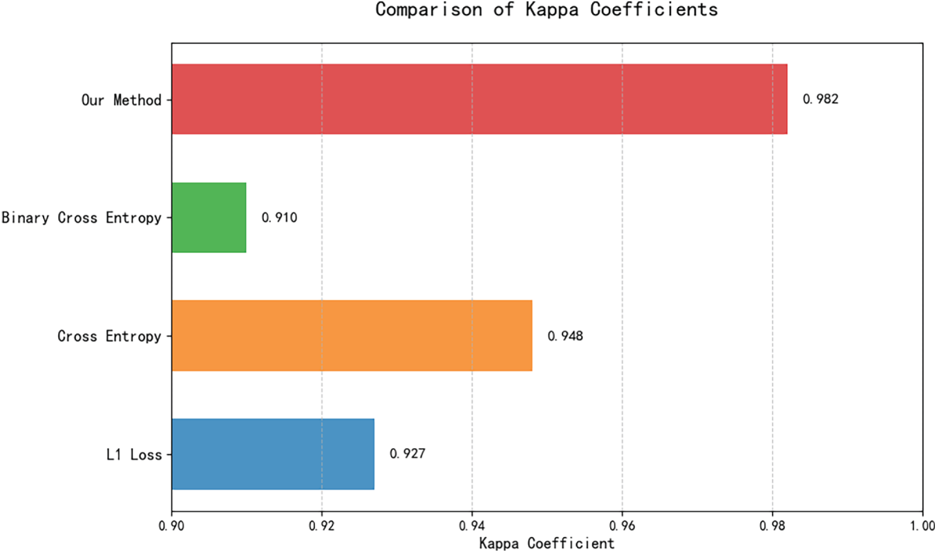
Figure 12: Transient stability assessment flowchart

Experimental results demonstrate that the proposed loss function achieves a higher Kappa coefficient compared to other loss functions, confirming its enhanced ability to learn minority class samples in imbalanced scenarios.

5.5 Noise Reduction Performance Analysis

5.5.1 Model Performance Analysis under Gaussian Noise

Tests were performed by injecting AWGN at SNRs of [30, 25, 20, 15 dB] into the experimental data. Simulations were carried out using the CSEE-DAS test case, and the results are illustrated in Fig. 13.

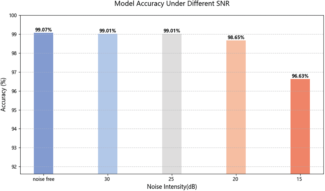
Figure 13: Visualization of classification performance under AWGN

As shown in Fig. 13, the classification accuracy of the proposed model experiences a slight decline as the SNR decreases. Nevertheless, even at an SNR of 15 dB, the model maintains a high accuracy of 96.63%, demonstrating its remarkable robustness under severe noise interference.

To further validate the noise immunity of the proposed model, comparative experiments were conducted against five other benchmark models under the same noisy conditions. The results are summarized in Table 4.

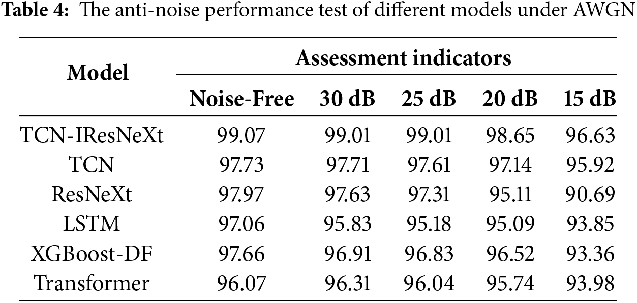
As evidenced by Table 4, the proposed TCN-ResNeXt model significantly outperforms all comparative models in terms of noise robustness, demonstrating superior stability and generalization capability in noisy environments.

5.5.2 Model Performance Analysis under Impulse Noise

The proposed classification assessment model was tested under impulse noise with SNRs set to [40, 30, 20 dB]. The experimental results are shown in Fig. 14.

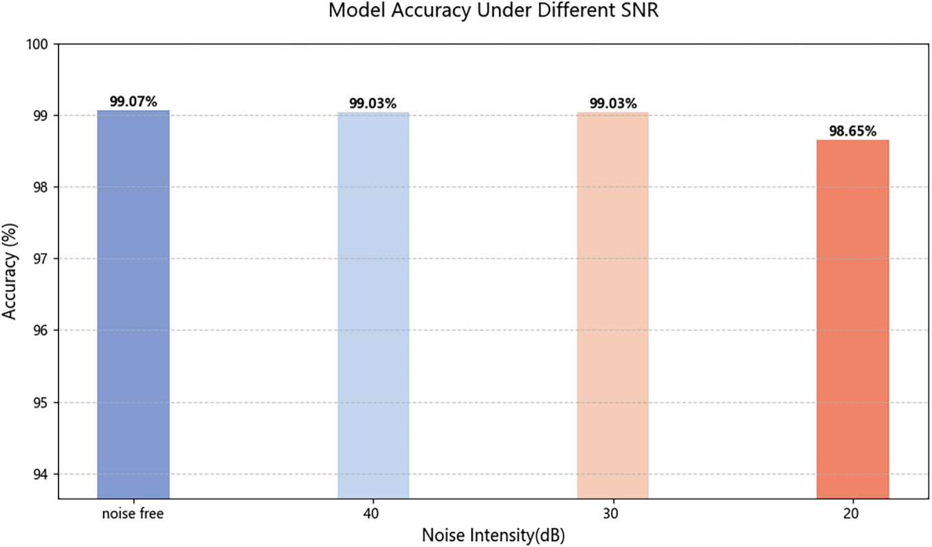
Figure 14: Visualization of classification performance under impulse noise

As shown in Fig. 14, the proposed model exhibits strong robustness against impulse noise, with only a minor decline in classification accuracy as the SNR decreases. Even at a low SNR of 20 dB, the model maintains a high accuracy of 98.65%. A comparative analysis was conducted with the five benchmark models listed in Table 5.

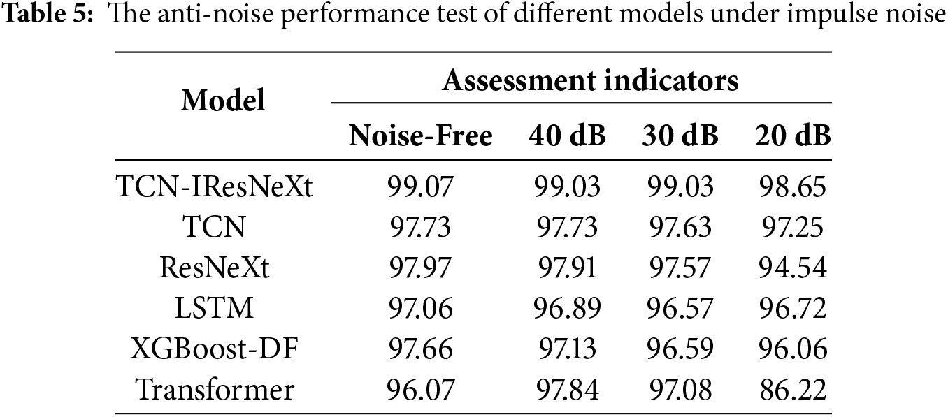
The noise immunity results under impulse noise conditions are summarized in Table 5. As clearly demonstrated in Table 5, the proposed classification assessment model significantly outperforms all comparative models in resisting impulse noise disturbances.

6  Conclusions

To enhance the evaluation performance of multi-class models under imbalanced sample conditions, a novel solution incorporating boundary sample loss is proposed. By leveraging the complementary strengths of TCN and IResNeXt, a hybrid multi-scale feature extraction network is constructed, which significantly enhances the accuracy of transient stability assessment for power systems. Extensive experiments conducted on both the CSEE-DAS and IEEE 140-bus systems validate the effectiveness of the proposed approach, with the main conclusions summarized as follows:

(1)   The designed TCN-IResNeXt multi-scale feature extraction network can dynamically extract comprehensive features spanning from local to global scales and both temporal and spatial dimensions. This design significantly enhances the model’s ability to represent and model complex power system data. Moreover, the incorporated attention mechanism dynamically focuses on critical features, thereby improving the physical interpretability of the model.

(2)   A solution for sample imbalance integrating boundary sample loss is proposed. This approach identifies boundary samples by evaluating the entropy of posterior probabilities and introduces a boundary loss term to increase the model’s cost sensitivity toward these critical samples. It effectively reduces the misdetection of unstable instances and further improves the classification accuracy for minority classes.

Although the model demonstrates superior performance in static and N-1 scenarios, its accuracy may degrade under substantial topological changes (e.g., simultaneous N-2 and N-3 outages). This performance profile clearly delineates the model’s capabilities: it excels in systems with localized perturbations but requires further enhancement to handle extensive topological changes effectively. Therefore, future work will focus on developing adaptive strategies, such as transfer learning-based model-updating mechanisms, to maintain strong generalization capability amid evolving grid conditions and significant topological reconfigurations.

Acknowledgement: Not applicable.

Funding Statement: This project is funded by the National Natural Science Foundation of China (5227-7084).

Author Contributions: The authors confirm contribution to the paper as follows: Study conception and design: Nan Li, Yinan Wang; data collection: Nan Li, Yinan Wang; analysis and interpretation of results: Nan Li, Yinan Wang, Liang Huang, Guangyao Zhang, Yabin Zhu; draft manuscript preparation: Nan Li, Yinan Wang. All authors reviewed the results and approved the final version of the manuscript.

Availability of Data and Materials: The datasets used and/or analyzed during the current study are available from the corresponding author upon reasonable request.

Ethics Approval: Not applicable.

Conflicts of Interest: The authors declare no conflicts of interest to report regarding the present study.

Appendix A

The CSEE_DASS test case nodes used in the simulation of this paper are shown in the figure below, and the test cases are built on the PSD Power System Simulation and Analysis Platform.

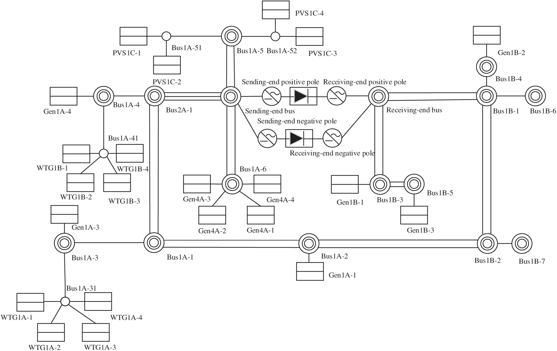
Figure A1: CSEE-DAS node graph

References

1. Xie L, Dong X, Lan Z. Evaluating the economic, security, and environmental values of renewable energy in the context of the new power system. In: Proceedings of the 2025 4th International Conference on New Energy System and Power Engineering (NESP); 2025 Apr 25–27; Fuzhou, China. p. 50–4. doi:10.1109/NESP65198.2025.11041604. [Google Scholar] [CrossRef]

2. Bi M, Fan H, Wang G, Fan Y, Li T, Ming H. Model-predictive-control based dispatching method for balancing resource in power grid. In: Proceedings of the 2023 5th International Conference on Smart Power & Internet Energy Systems (SPIES); 2023 Dec 1–4; Shenyang, China. p. 192–7. doi:10.1109/SPIES60658.2023.10475097. [Google Scholar] [CrossRef]

3. Shair J, Li H, Hu J, Xie X. Power system stability issues, classifications and research prospects in the context of high-penetration of renewables and power electronics. Renew Sustain Energy Rev. 2021;145:111111. doi:10.1016/j.rser.2021.111111. [Google Scholar] [CrossRef]

4. O’Sullivan J, Rogers A, Flynn D, Smith P, Mullane A, O’Malley M. Studying the maximum instantaneous non-synchronous generation in an island system—frequency stability challenges in Ireland. IEEE Trans Power Syst. 2014;29(6):2943–51. doi:10.1109/TPWRS.2014.2316974. [Google Scholar] [CrossRef]

5. Li W, Yang W, Zhang F, Wu S, Li Z. Extreme weather impact on carbon-neutral power system operation schemes: a case study of 2060 Sichuan province. Energy. 2024;313:133677. doi:10.1016/j.energy.2024.133677. [Google Scholar] [CrossRef]

6. Gao H, Jin T, Feng C, Li C, Chen Q, Kang C. Review of virtual power plant operations: resource coordination and multidimensional interaction. Appl Energy. 2024;357:122284. doi:10.1016/j.apenergy.2023.122284. [Google Scholar] [CrossRef]

7. Xiao D. A review on risk-averse bidding strategies for virtual power plants with uncertainties: resources, technologies, and future pathways. Technologies. 2025;13(11):488. doi:10.3390/technologies13110488. [Google Scholar] [CrossRef]

8. Lan J, Zhou Y, Guo Q, Sun H. A novel data-driven transient stability assessment of power systems based on uncertain data generation. In: Proceedings of the 2024 IEEE 7th International Electrical and Energy Conference (CIEEC); 2024 May 10–12; Harbin, China. p. 2973–8. doi:10.1109/CIEEC60922.2024.10583609. [Google Scholar] [CrossRef]

9. Xia S, Zhang C, Li Y, Li G, Ma L, Zhou N, et al. GCN-LSTM based transient angle stability assessment method for future power systems considering spatial-temporal disturbance response characteristics. Prot Control Mod Power Syst. 2024;9(6):108–21. doi:10.23919/PCMP.2023.000116. [Google Scholar] [CrossRef]

10. Massaoudi M, Zamzam T, Eddin ME, Ghrayeb A, Abu-Rub H, Refaat SS. Fast transient stability assessment of power systems using optimized temporal convolutional networks. IEEE Open J Ind Appl. 2024;5:267–82. doi:10.1109/OJIA.2024.3426334. [Google Scholar] [CrossRef]

11. Zhang L, An J, Zhou YB. Transient stability assessment of power system based on temporal convolution and graph attention network. Autom Electr Power Syst. 2023;47(7):114–22. (In Chinese). doi:10.7500/AEPS20220106003. [Google Scholar] [CrossRef]

12. Tan B, Yang J, Zhou T, Zhan X, Liu Y, Jiang S, et al. Spatial-temporal adaptive transient stability assessment for power system under missing data. Int J Electr Power Energy Syst. 2020;123:106237. doi:10.1016/j.ijepes.2020.106237. [Google Scholar] [CrossRef]

13. Zhan X, Han S, Rong N, Liu P, Ao W. A two-stage transient stability prediction method using convolutional residual memory network and gated recurrent unit. Int J Electr Power Energy Syst. 2022;138:107973. doi:10.1016/j.ijepes.2022.107973. [Google Scholar] [CrossRef]

14. Zhan X, Han S, Rong N, Cao Y. A hybrid transfer learning method for transient stability prediction considering sample imbalance. Appl Energy. 2023;333:120573. doi:10.1016/j.apenergy.2022.120573. [Google Scholar] [CrossRef]

15. Devi D, Biswas SK, Purkayastha B. Redundancy-driven modified Tomek-link based undersampling: a solution to class imbalance. Pattern Recognit Lett. 2017;93:3–12. doi:10.1016/j.patrec.2016.10.006. [Google Scholar] [CrossRef]

16. Krawczyk B, Koziarski M, Wozniak M. Radial-based oversampling for multiclass imbalanced data classification. IEEE Trans Neural Netw Learn Syst. 2020;31(8):2818–31. doi:10.1109/TNNLS.2019.2913673. [Google Scholar] [PubMed] [CrossRef]

17. Li N, Dong J, Tao L, Huang L. Transient stability assessment model and its updating based on dual-tower transformer. Energy Eng. 2025;122(7):2957–75. doi:10.32604/ee.2025.062667. [Google Scholar] [CrossRef]

18. Zhou X, Guan X, Sun D, Jiang H, Peng J, Jin Y, et al. Transient stability assessment based on gated graph neural network with imbalanced data in Internet of energy. IEEE Internet Things J. 2022;9(12):9320–31. doi:10.1109/JIOT.2021.3127895. [Google Scholar] [CrossRef]

19. Ouyang Y, Wang H. Adaptive denoising combined model with SDAE for transient stability assessment. Electr Power Syst Res. 2023;214:108948. doi:10.1016/j.epsr.2022.108948. [Google Scholar] [CrossRef]

20. Zhang T, Shen T, Hu G, Lu F, Du X. Stochastic reconstruction of digital cores using two-discriminator VAE-GAN. Geoenergy Sci Eng. 2024;236:212744. doi:10.1016/j.geoen.2024.212744. [Google Scholar] [CrossRef]

21. Yang M, Li Y, Li J, Lu G, Wang H, Fu Y, et al. Transfer learning-based updating method of transient stability assessment model. Energy Rep. 2024;12:442–52. doi:10.1016/j.egyr.2024.06.002. [Google Scholar] [CrossRef]

22. Li N, Zhang J. A transient stability assessment method of power system based on XGboost-DF. Electr Meas Instrum. 2024;61(10):119–27. (In Chinese). doi:10.19753/j.issn1001-1390.2024.10.016. [Google Scholar] [CrossRef]

23. Xie Z, Zhang D, Han X, Hu W. Power system transient stability preventive control optimization method driven by Stacking Ensemble Learning. Energy Rep. 2023;9:757–65. doi:10.1016/j.egyr.2023.05.106. [Google Scholar] [CrossRef]

24. Huang Y, Song Y, Cai Z. A supervised contrastive learning method with novel data augmentation for transient stability assessment considering sample imbalance. Reliab Eng Syst Saf. 2025;256:110716. doi:10.1016/j.ress.2024.110716. [Google Scholar] [CrossRef]

25. Li X, Liu C, Guo P, Liu S, Ning J. Deep learning-based transient stability assessment framework for large-scale modern power system. Int J Electr Power Energy Syst. 2022;139:108010. doi:10.1016/j.ijepes.2022.108010. [Google Scholar] [CrossRef]

26. Lea C, Vidal R, Reiter A, Hager GD. Temporal convolutional networks: a unified approach to action segmentation. In: Computer Vision—ECCV 2016 Workshops. Cham, Switzerland: Springer International Publishing; 2016. p. 47–54. doi:10.1007/978-3-319-49409-8_7. [Google Scholar] [CrossRef]

27. Xie S, Girshick R, Dollár P, Tu Z, He K. Aggregated residual transformations for deep neural networks. In: Proceedings of the 2017 IEEE Conference on Computer Vision and Pattern Recognition (CVPR); 2017 Jul 21–26; Honolulu, HI, USA. p. 5987–95. doi:10.1109/CVPR.2017.634. [Google Scholar] [CrossRef]

28. Misra D, Nalamada T, Arasanipalai AU, Hou Q. Rotate to attend: convolutional triplet attention module. In: Proceedings of the 2021 IEEE Winter Conference on Applications of Computer Vision (WACV); 2021 Jan 3–8; Waikoloa, HI, USA. p. 3138–47. doi:10.1109/WACV48630.2021.00318. [Google Scholar] [CrossRef]

29. Yang S, Li B, Hao Z, Hu Y, Xie H, Zhao T, et al. Multi-swing transient stability of synchronous generators and IBR combined generation systems. IEEE Trans Power Syst. 2025;40(1):1144–7. doi:10.1109/TPWRS.2024.3460421. [Google Scholar] [CrossRef]

30. Moon YH, Cho BH, Lee YH, Hong HS. Energy conservation law and its application for the direct energy method of power system stability. In: Proceedings of the IEEE Power Engineering Society. 1999 Winter Meeting; 1999 Jan 31–Feb 4; New York, NY, USA. p. 695–700. doi:10.1109/PESW.1999.747540. [Google Scholar] [CrossRef]

31. Devarapalli R, Bhattacharyya B. Power and energy system oscillation damping using multi-verse optimization. SN Appl Sci. 2021;3(3):383. doi:10.1007/s42452-021-04349-2. [Google Scholar] [CrossRef]

32. Li N, Zhu Y, Cui Y. AC-LSTM transient stability assessment considering cost-sensitivity. Power Syst Prot Control. 2022;50(22):160–9. (In Chinese). doi:10.19783/j.cnki.pspc.220217. [Google Scholar] [CrossRef]

33. Fang J, Liu C, Zheng L, Su C. A data-driven method for online transient stability monitoring with vision-transformer networks. Int J Electr Power Energy Syst. 2023;149:109020. doi:10.1016/j.ijepes.2023.109020. [Google Scholar] [CrossRef]