
 Login
Login Register
 Submit a Paper
 Propose a Special lssue
 Open Access
ARTICLE
Low-Carbon Economic Dispatch of a Virtual Power Plant Considering Concentrated Solar Power-Hydrogen Synergy and Asymmetric User Satisfaction
School of Intelligence Science and Technology, Xinjiang University, Urumqi, China
* Corresponding Author: Yue Meng. Email:
(This article belongs to the Special Issue: Integration of Renewable Energies with the Grid: An Integrated Study of Solar, Wind, Storage, Electric Vehicles, PV and Wind Materials and AI-Driven Technologies)
Energy Engineering 2026, 123(11), 21 https://doi.org/10.32604/ee.2026.083169
Received 30 March 2026; Accepted 08 June 2026; Issue published 24 September 2026
 View Full Text
 Download PDF
Abstract
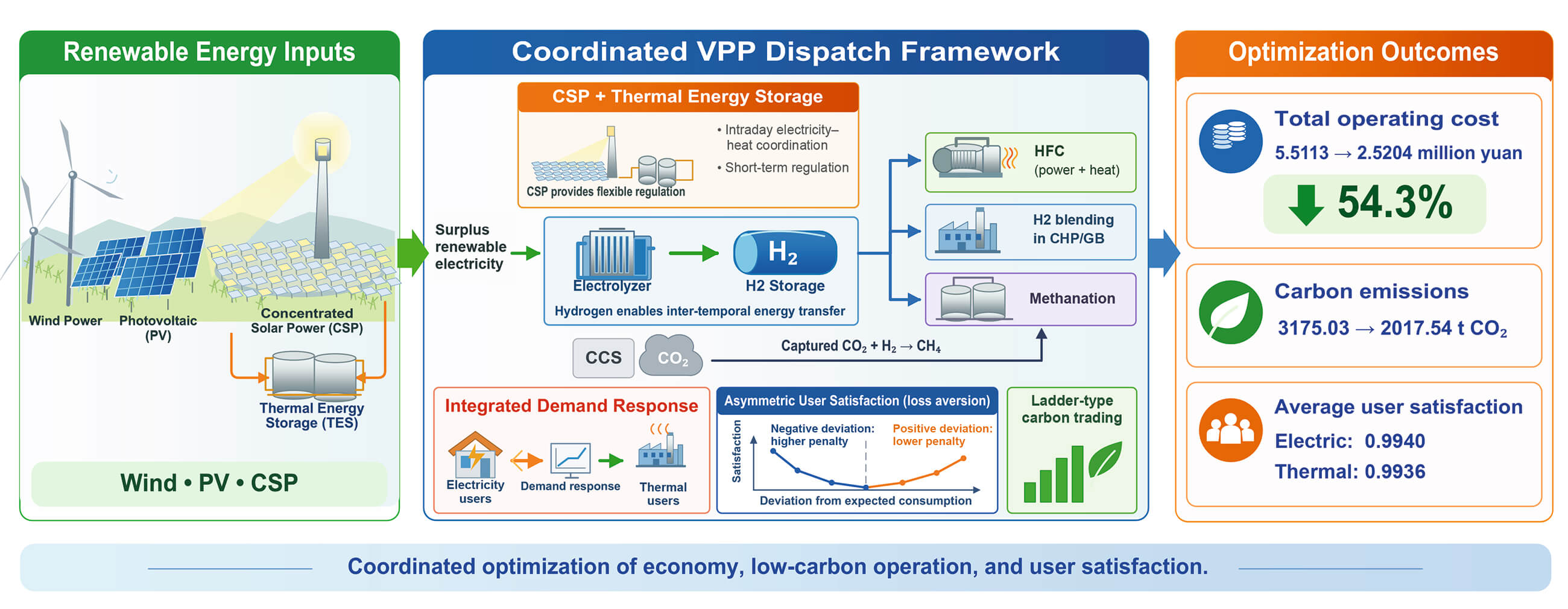
To address the difficulty of balancing economy, low-carbon performance, and user-side acceptability in virtual power plant operation under high penetration of renewable energy, this paper proposes a low-carbon optimal dispatch model for a virtual power plant considering concentrated solar power (CSP)-hydrogen synergy and asymmetric user satisfaction. First, a coordinated operation model of CSP and hydrogen energy is established by incorporating a CSP plant, hydrogen conversion devices, hydrogen-blended gas equipment, and multiple types of energy storage systems into a unified dispatch framework. Second, to overcome the limitation of conventional user satisfaction models in reflecting users’ differentiated perceptions of load deviations in different directions, an asymmetric user satisfaction model is developed based on loss aversion theory. Combined with an integrated demand response mechanism, the proposed model improves the rationality of user response characterization. On this basis, a ladder-type carbon trading mechanism is introduced, and an optimal dispatch model is established with the objective of minimizing the total operating cost over the scheduling horizon while simultaneously considering economy, low-carbon performance, and user satisfaction. Case study results show that, compared with the baseline operating scenario, the proposed model reduces the total operating cost by 54.3% and significantly decreases carbon emissions. Compared with the conventional symmetric user satisfaction model, the average satisfaction levels of both electric and thermal loads are improved, with a more pronounced enhancement observed for thermal loads. The results demonstrate that the proposed model can achieve coordinated optimization of low-carbon operation, economic dispatch, and user satisfaction while satisfying users’ basic energy demands.Graphic Abstract
Keywords
Under the ongoing push toward the “dual-carbon” goals and the development of new-type power systems, the installed capacity of renewable energy sources such as wind power and photovoltaics has continued to grow. However, the volatility, intermittency, and uncertainty of renewable generation have imposed greater challenges on secure and stable system operation as well as on system security, stability, and operational flexibility [1]. By aggregating distributed generators, energy storage devices, and flexible loads through advanced information and communication technologies, coordinated control, and optimal dispatch, virtual power plants (VPPs) can effectively exploit demand-side flexibility, improve renewable energy accommodation, and promote the transition of power systems from a traditional “generation-following-load” mode to a more interactive “source-load coordination” paradigm [2,3]. With the development of integrated energy technologies, the scope of VPP research has gradually expanded from the aggregation of conventional electric resources to multi-energy coordinated systems involving electricity, heat, gas, and hydrogen. Under such a multi-energy coupling framework, how to balance economic performance, low-carbon operation, and dispatch flexibility has become an important research issue.
Against this backdrop, CSP and hydrogen utilization provide new flexibility resources for multi-energy-coupled VPPs. Supported by thermal energy storage, CSP plants are well suited to intraday electricity-heat coordination and short-term peak shaving. By contrast, hydrogen systems enable inter-temporal energy transfer and long-duration storage through water electrolysis, hydrogen storage, and hydrogen utilization. These two technologies are highly complementary in both the regulation timescale and the energy utilization mode. Incorporating them into a unified VPP dispatch framework is therefore conducive to enhancing multi-energy coordinated operation and improving renewable energy utilization.
Considerable efforts have been made to investigate low-carbon optimal dispatch in multi-energy-coupled VPPs from different perspectives. Ref. [4] developed an optimal dispatch model for a VPP with P2G-CCS coupling and hydrogen blending under a ladder-type carbon trading mechanism, showing that hydrogen utilization and carbon recycling can improve low-carbon operation. Ref. [5] examined the optimal operation of an electricity-heat energy system including a CSP plant and pointed out that the thermal storage unit of CSP can strengthen electricity-heat coordination and peak regulation capability. Ref. [6] combined demand response with a ladder-type carbon trading mechanism and verified that the coordinated use of low-carbon market mechanisms and load-side regulation can effectively reduce both operating cost and carbon emissions. Ref. [7] further incorporated diversified hydrogen utilization into a low-carbon dispatch framework and analyzed its impact on system economy, carbon performance, and flexibility. Overall, existing studies have separately addressed the thermal storage regulation capability of CSP plants, the inter-temporal energy transfer capability of hydrogen systems, and the effects of carbon trading and demand response on system operation. However, the coordinated operation of CSP and hydrogen systems within a unified VPP framework has received relatively limited attention. In particular, the complementary relationship between CSP and hydrogen systems in terms of regulation timescale and energy utilization mode still lacks systematic modeling and coordinated optimization analysis.
In demand response modeling, increasing attention has also been paid to the behavioral characteristics of flexible user-side resources. Ref. [8] established an optimal VPP dispatch model based on refined demand response and characterized the response behaviors of different types of users, showing that a more detailed description of demand response resources and user response characteristics can improve both economic performance and operational flexibility. Ref. [9] investigated data-driven methods for modeling user demand response behavior, providing support for a more refined representation of flexible demand-side resources. Ref. [10] introduced a user satisfaction index into integrated demand response optimization to limit the adverse impacts of excessive adjustment on users’ energy-use experience. Ref. [11] further incorporated carbon emission trading and user satisfaction into the VPP optimal dispatch framework, thereby accounting for user-side acceptability while pursuing low-carbon operation. Nevertheless, most existing satisfaction models focus on static evaluations of comfort, compensation level, or aggregate utility, and remain limited in capturing users’ heterogeneous behavioral perceptions during demand response. In practice, users generally do not perceive load reduction and load compensation symmetrically. If satisfaction is still modeled in a symmetric manner, the sensitivity of users to negative load deviations may be underestimated, which weakens the model’s characterize actual response willingness and feasible response boundaries.
From the perspective of behavioral mechanisms, behavioral economics provides a useful theoretical basis for user response modeling in demand response. Ref. [12] pointed out that users responding to incentive signals do not always behave in a fully rational manner; instead, their decisions are often influenced by reference dependence and loss aversion. According to prospect theory as proposed in Ref. [13], decision-makers generally perceive losses more strongly than equivalent gains, implying that user acceptance may differ significantly across different directions of load deviation. Demand response is therefore not merely a process of load adjustment driven by price signals, but is also closely related to users’ behavioral perceptions. However, within the existing VPP optimal dispatch literature, relatively few studies have incorporated such asymmetric perceptions arising from loss aversion into user satisfaction modeling, or further coupled them with CSP-hydrogen coordinated operation and ladder-type carbon trading.
To address the above issues, this paper investigates the low-carbon economic dispatch of a VPP. First, CSP plants and hydrogen utilization units are jointly incorporated into a unified optimal dispatch framework of the VPP, and their complementary roles in regulation time scale, power regulation, and energy utilization mode are analyzed to characterize the coordinated operation of the system under multi-energy coupling. Second, considering that users perceive load deviations in different directions differently, an asymmetric user satisfaction model is introduced into demand response modeling to improve the realism of user response characterization. Finally, the ladder-type carbon trading mechanism is coupled with the multi-energy coordinated dispatch process to establish an optimal dispatch model that simultaneously considers economic performance, low-carbon operation, and user satisfaction. The results of this study can provide a useful reference for the low-carbon optimal dispatch of multi-energy-coupled VPPs.
2 VPP Framework Incorporating Demand Response and Asymmetric User Satisfaction
As shown in Fig. 1, the VPP framework developed in this study comprises five parts: upstream energy supply, multi-energy coupling, energy storage, end-use demand, and carbon capture with carbon constraints. On the demand side, the system includes electric and thermal loads. On the supply side, it integrates wind power, photovoltaic generation, a CSP plant, a combined heat and power (CHP) unit, a gas boiler (GB), a hydrogen fuel cell (HFC), and the upper-level power grid and natural gas network. To balance energy supply and demand and improve operational flexibility, electrical, thermal, and hydrogen storage systems are incorporated in the system.
In terms of energy conversion, renewable energy provides clean electricity for the VPP. Surplus electricity is converted into hydrogen through an electrolyzer. The produced hydrogen can be used directly in the HFC for CHP generation, or it can react with captured carbon dioxide in a methanation reactor to produce synthetic natural gas, which is then injected into the natural gas system. In this way, cascade utilization of hydrogen and recycling of carbon resources can be achieved. In addition, the CHP unit and gas boiler meet electricity and heat demand by consuming hydrogen-blended natural gas, which helps reduce the carbon intensity of energy supply. The consumption of fossil energy, together with carbon dioxide emissions and capture processes, is incorporated into a unified carbon-constrained framework, providing the basis for the low-carbon economic dispatch model developed in this paper.
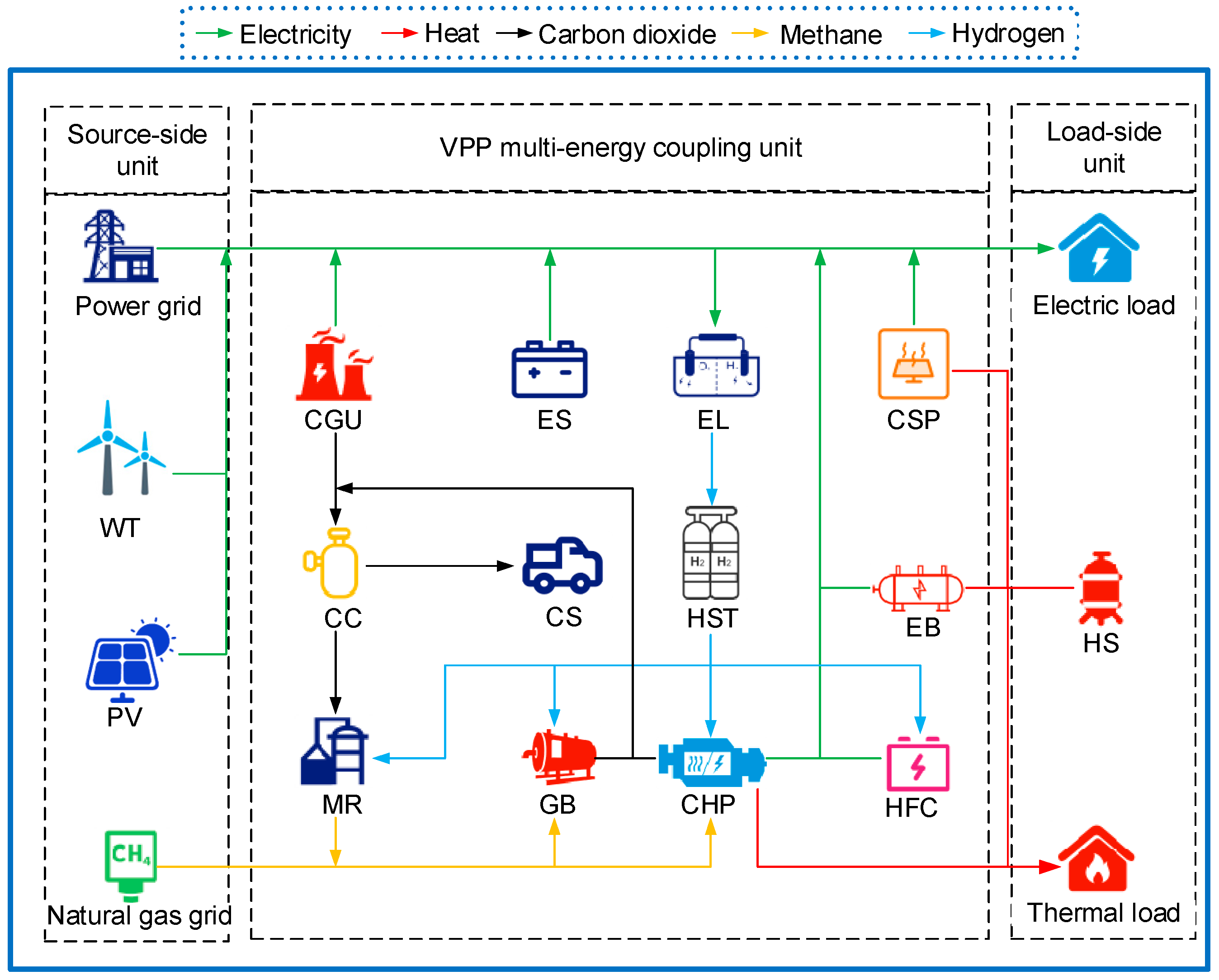
Figure 1: Schematic diagram of the virtual power plant system.
Demand response refers to the proactive adjustment of users’ energy consumption behavior under price signals or incentive mechanisms to reshape load profiles and improve system operational flexibility. Considering the regulation characteristics of electric and thermal loads in the virtual power plant, demand response in this paper is divided into two categories: price-based demand response and substitution-based demand response [14]. To characterize the flexibility of different loads, both electric and thermal loads are further classified into fixed loads, transferable loads, reducible loads, and substitutable loads. Among them, fixed loads do not participate in regulation; transferable loads can be shifted across different time periods; reducible loads can be curtailed within specified limits; and substitutable loads can be replaced through energy conversion between different energy forms. Based on this classification, price-based demand response and substitution-based demand response models are established, respectively.
2.1.1 Price-Based Demand Response Model
Price-based demand response mainly describes users’ load-shifting and load-curtailment behavior in response to price signals. In this paper, a demand price elasticity matrix is employed to characterize the sensitivity of loads to price variations [15]. The demand price elasticity matrix is denoted by
The transferable response amounts and reducible response amounts of electric and thermal loads are expressed as follows, respectively:
2.1.2 Substitution-Based Demand Response Model
Substitution-based demand response mainly describes users’ adjustment of energy consumption patterns under different energy price conditions, thereby enabling mutual substitution between electric and thermal loads [16]. Let
When
2.1.3 Integrated Demand Response Model
After jointly considering price-based demand response and substitution-based demand response, the electric load and thermal load after demand response can be expressed as follows, respectively:
2.2 Asymmetric User Satisfaction Model
During demand response, load adjustment can improve system operational flexibility, but excessive load deviation may adversely affect users’ energy-use experience. Therefore, user satisfaction constraints are introduced into the optimal dispatch model to prevent excessive adjustment from adversely affecting user-side energy-use experience [17]. Most existing satisfaction models treat the effects of load deviation on user experience symmetrically, which makes it difficult to reflect users’ differentiated perceptions of load deviations in different directions. In practice, when the adjusted load level is lower than the original demand level, users tend to exhibit stronger dissatisfaction; by contrast, when the adjusted load level exceeds the original demand level, the resulting negative perception is usually weaker. Based on this observation, this paper develops an asymmetric user satisfaction model grounded in loss aversion theory, and uses differentiated weighting factors to characterize the different effects of positive and negative deviations on user perception.
Let
On this basis, the user satisfaction levels for electric load and thermal load are defined as follows:
To ensure that users’ basic energy demand is satisfied, lower-bound constraints on user satisfaction are further imposed as follows:
The parameters in the asymmetric user satisfaction model are mainly used to characterize users’ differentiated perceptions of load deviations in different directions. Specifically, the positive deviation penalty coefficient is used to describe the variation in user satisfaction when the actual load is higher than the original load, while the negative deviation penalty coefficient is used to characterize the satisfaction loss when the actual load is lower than the original load. According to loss aversion theory, users are generally more sensitive to load reduction or insufficient energy supply than to load increase. Therefore, the negative deviation penalty coefficient is set larger than the positive deviation penalty coefficient in this paper. The minimum user satisfaction threshold is introduced to ensure the basic energy-use experience of users after demand response. Considering that industrial park users differ in production processes, energy-use continuity, and response willingness, it is difficult to represent the relevant parameters using unified fixed values. Therefore, the parameter settings in this paper are mainly determined by referring to existing demand response studies and considering the load regulation characteristics of industrial parks. In the case study, the positive deviation penalty coefficients for electric and thermal loads are both set to 0.08, the negative deviation penalty coefficients are both set to 0.15, and the minimum user satisfaction threshold is set to 0.85.
To further quantify the impact of demand response on users’ energy-use experience, user satisfaction loss is converted into an economic penalty cost and incorporated into the objective function. Considering that electric and thermal loads may exhibit different sensitivities to satisfaction variations, the satisfaction penalty cost is defined as follows:
3 Ladder-Type Carbon Trading Mechanism Model
Carbon trading allocates carbon emission rights through market-based mechanisms and guides emission entities to actively reduce their carbon emissions. It is an important means of achieving low-carbon system operation. In this paper, the carbon trading mechanism model is established from three aspects, namely the initial carbon emission allowance, actual carbon emissions, and ladder-type carbon trading cost [18].
3.1 Initial Carbon Emission Allowance Model
In the current carbon trading market, the initial carbon emission allowance is usually allocated based on the benchmark method. Considering the operational structure of the virtual power plant, electricity purchased from the upper-level grid, the CHP unit, the gas boiler, the coal-fired unit, and natural gas consumption are regarded as the main sources of carbon emissions within the carbon accounting boundary of the VPP. Therefore, the total initial carbon emission allowance of the system over the scheduling horizon can be expressed as follows:
3.2 Actual Carbon Emission Model
Considering that grid-purchased electricity, the CHP unit, the GB, the coal-fired unit, and natural gas consumption within the carbon accounting boundary of the system all contribute to carbon emissions, while the CCS unit can capture a portion of CO2 emissions, the actual carbon emission model of the system can be expressed as follows:
To further clarify the CO2 flow boundary of the system, Fig. 2 illustrates the CO2 flow boundary of the system. The direct CO2 emissions within the system mainly originate from the CHP unit, gas boiler, and coal-fired unit. Among them, the CO2 emissions from the CHP unit and gas boiler are determined by the natural gas input in the mixed fuel, whereas hydrogen combustion does not directly generate CO2. The CO2 emissions associated with electricity purchased from the upper-level grid are regarded as external indirect emissions and are not involved in the local CCS capture process.
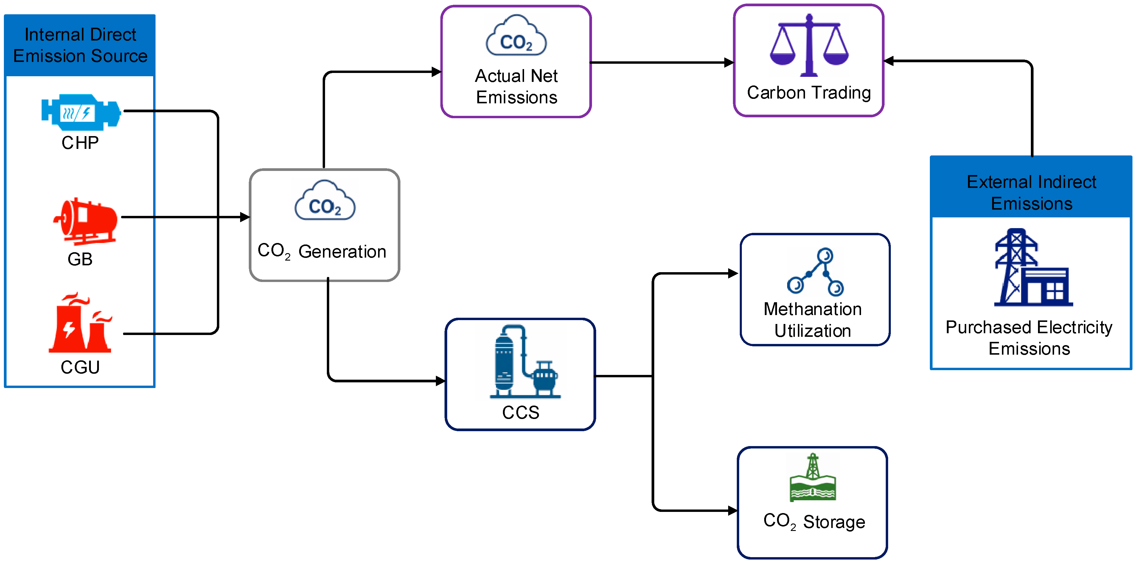
Figure 2: Schematic diagram of system CO2 flow boundary.
Part of the locally generated CO2 is captured by CCS and then supplied to the methanation reactor, where it reacts with H2 produced by the electrolyzer to synthesize CH4, thereby realizing CO2 resource utilization. Another part of the captured CO2 is transferred to the storage process, while the CO2 that is not captured or treated is regarded as the actual net emissions of the system. These net emissions are compared with the initial carbon allowance to calculate the carbon trading cost. The CO2 used for methanation is considered an internal destination of captured CO2 and is therefore not repeatedly deducted as an additional emission reduction.
3.3 Ladder-Type Carbon Trading Cost Model
To reflect both the penalty for excess carbon emissions and the revenue from surplus carbon allowances, a ladder-type carbon trading mechanism is introduced based on the benchmark carbon price. The deviation between the actual carbon emissions and the initial carbon emission allowance is divided into different intervals, and the carbon trading cost is calculated in a piecewise manner with increasing marginal prices. When the emission deviation is negative, it indicates that the system has surplus carbon allowances and can obtain revenue by selling the remaining allowances. The ladder-type carbon trading cost model is given as follows:
4.1 Constraints of the CSP Plant Model
The CSP plant mainly consists of three subsystems, namely solar collection, thermal energy storage, and power generation, and uses heat transfer fluid (HTF) as the medium for energy transfer to realize internal heat transfer and energy conversion. Considering that the CSP plant in this study simultaneously undertakes electricity and heat supply, its internal energy flow and coupling relationships are further established, as shown in Fig. 3.
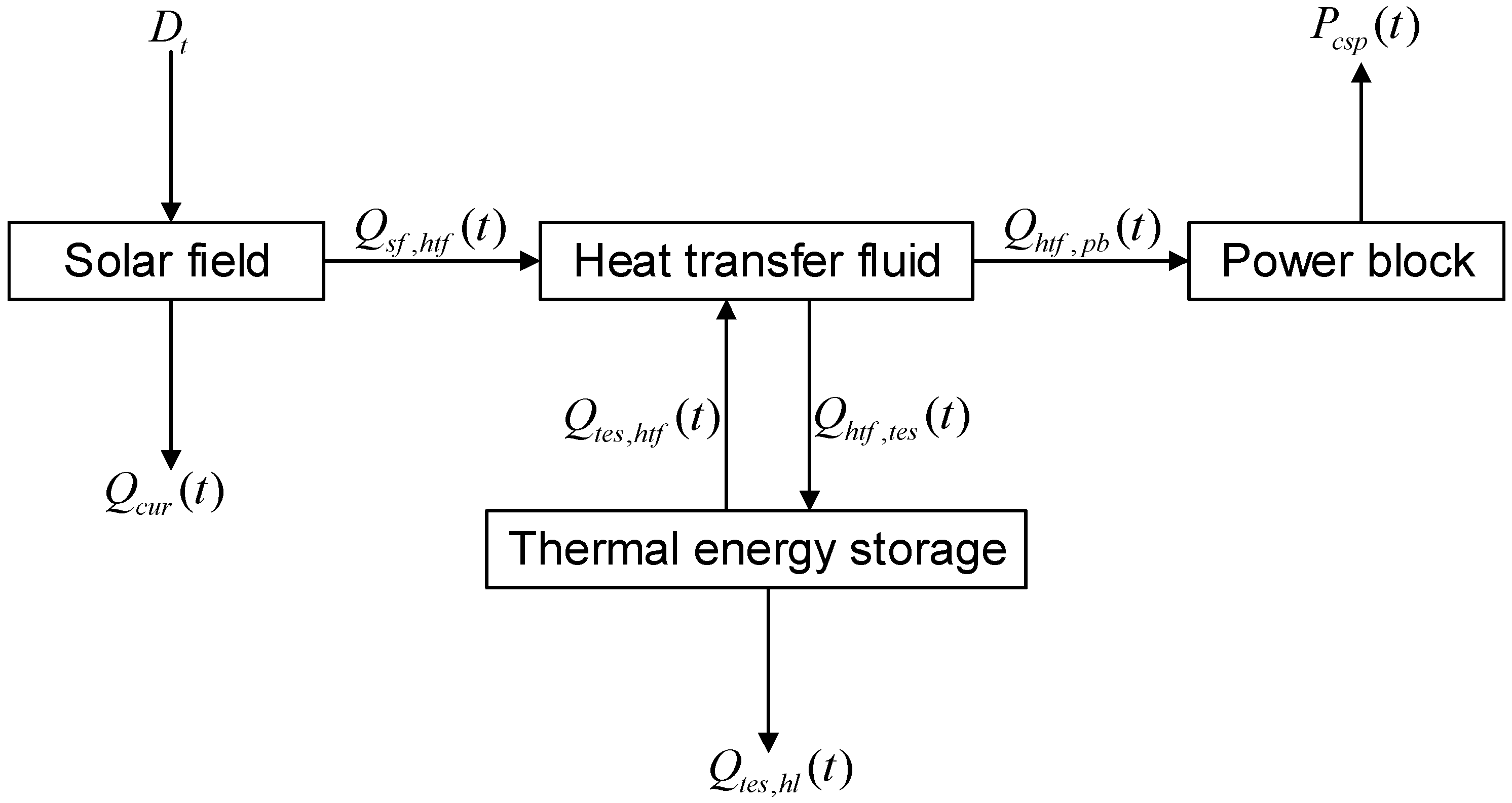
Figure 3: Schematic diagram of internal energy flow in CSP plant.
According to the internal energy transfer process of the CSP plant, its operation model can be divided into four stages: solar collection, heat transfer, thermal charging/discharging, and power generation [19].
- (1)Solar collection stage
- (2)Heat transfer stage
- (3)Thermal charging/discharging stage
- (4)Power generation stage
The power generation stage is modeled with the steam turbine as the core component, while considering output limits, ramp-rate limits, and start-up/shut-down constraints. The mathematical formulation is given as follows:
4.2 Wind Turbine Output Constraint
The constraint is expressed as follows:
4.3 Photovoltaic Unit Output Constraint
The constraint is expressed as follows:
4.4 Coal-Fired Unit Operating Constraints
As a conventional power generation unit in the system, the coal-fired unit is required to satisfy the upper and lower limits of power output as well as ramping constraints during the scheduling horizon [20]:
4.5 Constraints of the Electric Boiler Model
The electric boiler (EB) generates heat by consuming electricity, and its operating constraints can be expressed as follows:
4.6 Constraints of the Diversified Hydrogen Utilization Model
As a clean and efficient secondary energy carrier, hydrogen can enhance the system’s multi-energy coupling capability and inter-temporal regulation flexibility. In this paper, a hydrogen production and diversified utilization module composed of the electrolyzer, methanation reactor, carbon capture unit, HFC, and hydrogen-blended gas equipment is established to realize flexible conversion among electricity, hydrogen, gas, and heat.
- (1)Electrolyzer model
The electrolyzer (EL) converts input electricity into hydrogen. Its operating constraints include the conversion relationship between hydrogen production and input electric power, as well as the upper and lower bounds and ramping constraints of the EL input power, which can be expressed as follows:
- (2)Methanation reactor model
The methanation reactor (MR) synthesizes natural gas by using hydrogen produced by the electrolyzer and CO2 captured by the CCS unit. Its operating constraints include the natural gas output, CO2 consumption, and the upper and lower bounds and ramping constraints of the MR input power, which can be expressed as follows:
- (3)Carbon capture and storage model
To reduce the carbon emission level of the system, a carbon capture and storage (CCS) unit is introduced in this paper. The relationship between the carbon capture amount and the operating energy consumption can be expressed as follows:
- (4)Hydrogen fuel cell model
The HFC can convert the chemical energy of hydrogen into electric energy and simultaneously release part of the thermal energy. Its energy conversion relationship can be expressed as follows:
- (5)Hydrogen-blended gas turbine model
The hydrogen-blended gas turbine is an important device for realizing the coupled conversion of electricity, gas, and heat in the system. In this paper, its hydrogen-blended operation model is established with reference to Ref. [21] to characterize the power generation, heat supply, and hydrogen blending ratio constraints under natural gas–hydrogen mixed combustion conditions.
- (6)Hydrogen-blended gas boiler model
After the introduction of hydrogen blending technology, the gas boiler can further improve the flexibility of heat supply and reduce fossil energy consumption. In this paper, the hydrogen-blended gas boiler model is established with reference to Ref. [21], and its mathematical formulation is given as follows:
4.7 Energy Storage Operating Constraints
To enhance the system’s capability for inter-temporal energy regulation, electrical energy storage, the system-side thermal storage tank, and the hydrogen storage device are modeled in a unified manner in this paper [22].
- (1)Electric power balance constraint
The electric power balance of the system can be expressed as follows:
- (2)Thermal power balance constraint
The thermal power balance of the system can be expressed as follows:
- (3)Natural gas balance constraint
The natural gas balance of the system can be expressed as follows:
- (4)Hydrogen balance constraint
The hydrogen balance of the system can be expressed as follows:
To simultaneously consider system economy, low-carbon performance, and user-side response behavior, an optimization model is established in this paper with the objective of minimizing the total operating cost of the virtual power plant over the scheduling horizon:
- (1)Coal-fired unit cost
- (2)Carbon capture, storage, and trading cost
- (3)Wind and photovoltaic curtailment penalty cost
- (4)Electricity purchase cost
- (5)Natural gas purchase cost
- (6)Demand response and satisfaction penalty cost
- (7)CSP plant cost
To verify the effectiveness and feasibility of the proposed model and operating strategy, a case study is designed in this paper with a 24 h scheduling horizon and a 1 h basic scheduling interval. The electric and thermal load curves, as well as the renewable energy output profiles including wind power and photovoltaics, are shown in Fig. 4. The main parameter settings are as follows: the time-of-use electricity price is given in Table 1, and the natural gas price is set to 0.35 yuan/kWh. The equipment parameters are listed in Table 2. For the carbon trading mechanism, the benchmark carbon price is set to 215 yuan/t, the step length of each carbon trading interval is 50 t, the growth rate of the carbon trading price is 25%, and the unit carbon storage cost is 50 yuan/t. Based on historical operating experience and the load regulation characteristics of the industrial park, the proportions of reducible, transferable, and substitutable loads in both electric and thermal loads are set to 25%, 10%, and 5% of the total load, respectively.
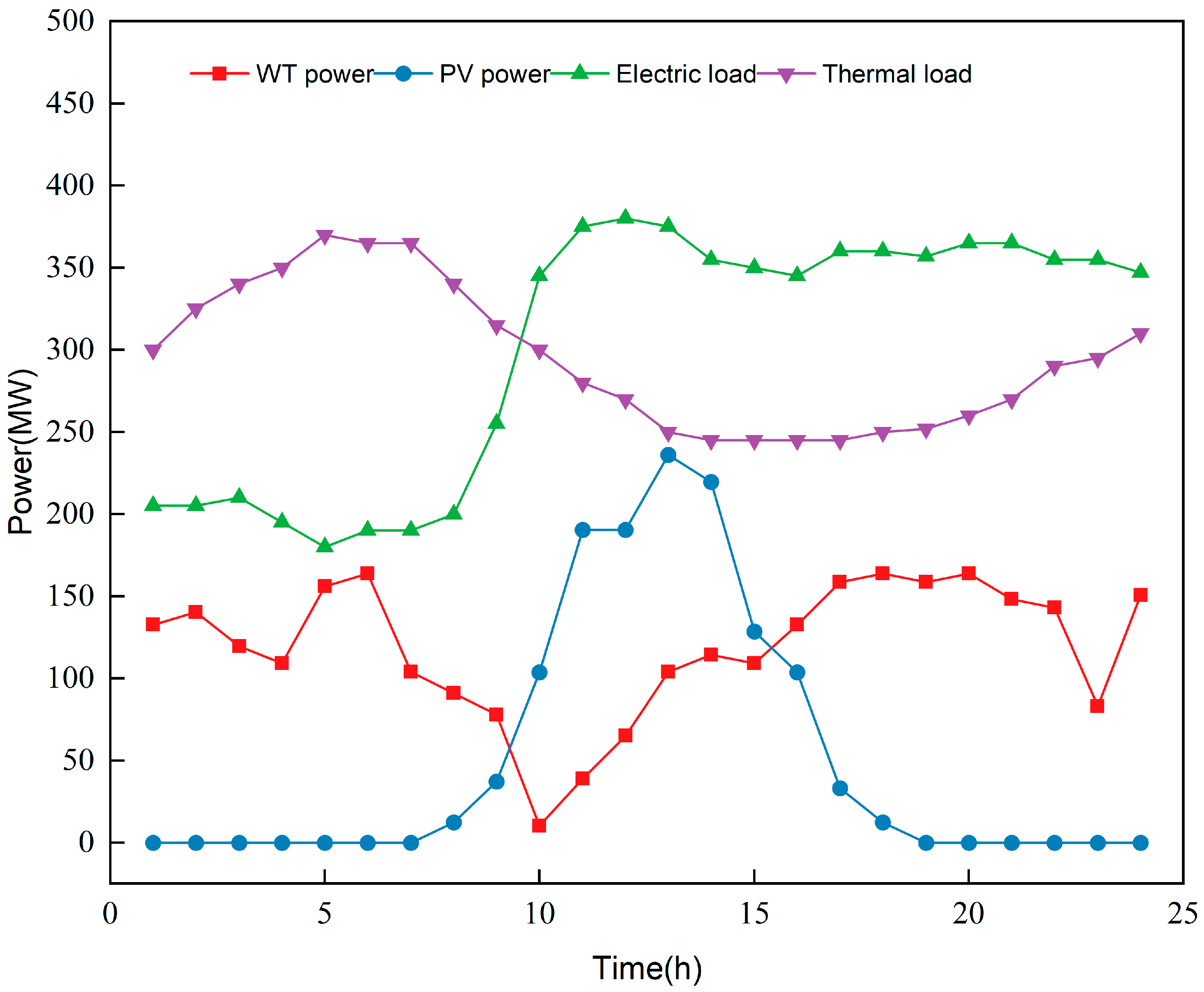
Figure 4: Load and renewable energy output curves.
Table 1: Time-of-use electricity prices.
| Time Period | Electricity Price (yuan) |
|---|---|
| 00:00–07:00 | 0.4438 |
| 08:00–14:00, 19:00–22:00 | 0.8118 |
| 15:00–18:00, 23:00–24:00 | 0.5713 |
Table 2: Operating parameters of each equipment.
| Device | Parameter | Value |
|---|---|---|
| CHP | Maximum/Minimum electric power output (MW) | 350/0 |
| Maximum/Minimum heat output power (MW) | 300/0 | |
| Total ramp-up/ramp-down limits (MW/h) | 150/−150 | |
| Heat-to-electric efficiency | 0.40/0.35 | |
| GB | Maximum/Minimum heat output power (MW) | 80/0 |
| Heat output ramp-up/ramp-down limits (MW/h) | 25/−25 | |
| Conversion efficiency | 0.92 | |
| EB | Maximum/Minimum electric power consumption (MW) | 40/0 |
| Electric power ramp-up/ramp-down limits (MW/h) | 10/−10 | |
| Conversion efficiency | 0.90 | |
| TH | Maximum/Minimum electric power output (MW) | 160/0 |
| Electric power ramp-up/ramp-down limits (MW/h) | 100/−100 | |
| P2G | Power-to-hydrogen efficiency | 0.85 |
| Maximum/Minimum electric power consumption (MW) | 120/0 | |
| Methanation efficiency | 0.7 | |
| HFC | Maximum/Minimum electric power output (MW) | 50/0 |
| Maximum/Minimum heat output power (MW) | 30/0 | |
| Output ramp-up/ramp-down limits (MW/h) | 15/−15 | |
| Heat-to-electric efficiency | 0.5/0.3 | |
| CSP | Solar collection efficiency | 0.3 |
| Power generation efficiency | 0.4 | |
| Thermal storage efficiency | 0.9 | |
| Power output range (MW) | 150/0 |
5.2 Benefit Analysis of Different Operating Strategies
To verify the effectiveness of the proposed VPP model and to analyze the impact of different functional modules on the operation results of the VPP, six progressive operating scenarios and one additional ablation scenario are designed for comparative analysis under the same load data, renewable energy output, energy prices, equipment capacity limits, and operating constraints. These scenarios are constructed by gradually introducing different functional modules, and Scenario 6 represents the complete dispatch model proposed in this paper. Scenario 7 is designed as an additional ablation scenario and is mainly used in the subsequent CSP–hydrogen coordinated operation analysis to further quantify the independent and combined effects of the CSP plant and the hydrogen energy chain. The settings of each scenario are as follows:
Scenario 1: A conventional VPP optimal operation model is established as the benchmark case.
Scenario 2: A CSP plant is introduced into the conventional VPP model.
Scenario 3: A P2G-CCS system is further introduced on the basis of Scenario 2.
Scenario 4: Hydrogen blending equipment and fuel cell units are introduced on the basis of Scenario 3.
Scenario 5: Demand response and user satisfaction modules are introduced on the basis of Scenario 4.
Scenario 6: An asymmetric user satisfaction model is further introduced on the basis of Scenario 5.
Scenario 7: A complete hydrogen energy chain, including P2G-CCS, hydrogen fuel cells, and hydrogen blending, is introduced based on Scenario 1, without introducing the CSP plant.
Table 3 presents the optimal dispatch results of the VPP under different operating scenarios. Overall, with the gradual introduction of system functional modules, the operational economy of the VPP is significantly improved, and the complete model achieves the best performance in terms of carbon emission control. From Scenario 1 to Scenario 6, the total operating cost decreases from 5.5113 million yuan to 2.5204 million yuan, representing a reduction of 54.3%, while carbon emissions decrease from 3175.03 t to 2017.54 t. This indicates that, under the case-study conditions of this paper, multi-energy coupling and demand-side coordinated optimization can improve the overall operational performance of the system. It should be noted that the effects of different functional modules on the total carbon emissions of the system are not strictly monotonic. In some intermediate scenarios, phased fluctuations in carbon emissions may occur due to factors such as the output of coal-fired units, grid-purchased electricity, the power source for hydrogen production, and the amount of CO2 captured by CCS.
Table 3: Comparison of optimal scheduling results for Scenarios 1–7.
| Scenario 1 | Scenario 2 | Scenario 3 | Scenario 4 | Scenario 5 | Scenario 6 | Scenario 7 | |
|---|---|---|---|---|---|---|---|
| Total cost | 5,511,275.32 | 3,203,007.70 | 2,785,108.65 | 2,744,643.77 | 2,583,592.01 | 2,520,357.65 | 4,685,012.5 |
| Coal unit cost | 298,565.62 | 353,983.94 | 338,458.65 | 448,465.58 | 435,644.95 | 376,138.43 | 375,340.72 |
| Carbon cost | 221,914.88 | 219,548.95 | 163,300.52 | 233,225.74 | 255,100.81 | 173,646.76 | 294,924.81 |
| Curtailment penalty | 435,133.40 | 58,014.22 | 5130.00 | 0 | 0 | 0 | 29,519.09 |
| Gas purchase cost | 4,517,745.05 | 2,232,774.40 | 1,974,780.44 | 1,753,928.14 | 1,384,785.59 | 1,543,567.53 | 3,985,227.9 |
| Power purchase cost | 37,916.37 | 50,603.60 | 26,051.28 | 55,359.35 | 15,179.36 | 13,308.19 | 0 |
| DR & satisfaction cost | - | - | - | - | 235,348.19 | 127,871.98 | - |
| CSP cost | - | 288,082.59 | 277,387.76 | 253,664.96 | 257,533.10 | 285,824.77 | - |
| Carbon emissions | 3175.03 | 2204.14 | 2045.70 | 2475.80 | 2310.26 | 2017.54 | 3785.02 |
| Avg. electric satisfaction | - | - | - | - | 0.97435 | 0.99404 | - |
| Avg. thermal satisfaction | - | - | - | - | 0.88547 | 0.99361 | - |
After the CSP plant is introduced in Scenario 2, the total operating cost of the system decreases significantly compared with Scenario 1, and the penalty cost for wind and photovoltaic curtailment is substantially reduced. This is because the CSP plant has flexible heat supply and thermal storage capabilities, which can alleviate the conventional electricity–heat coupling constraints, improve the coordinated operation of electricity and heat, enhance wind and photovoltaic power accommodation, and reduce part of the external energy purchase demand.
After the P2G-CCS system is further introduced in Scenario 3, both the total operating cost and carbon emissions of the system continue to decrease. The P2G unit can convert surplus wind and photovoltaic power into hydrogen during periods of renewable energy surplus and realizes electricity–gas coupling and CO2 resource utilization through the methanation process. As a result, the system’s gas purchase demand is reduced and its low-carbon operation capability is enhanced.
After hydrogen blending and fuel cells are introduced in Scenario 4, the system forms a hydrogen utilization chain of “hydrogen production–hydrogen storage–hydrogen consumption”. Hydrogen can be used not only for methanation and hydrogen blending in gas-fired equipment, but also for combined heat and power generation through fuel cells. This further improves system flexibility, enhances renewable energy accommodation, and reduces dependence on conventional fossil energy. It should be noted that hydrogen blending mainly reduces the direct carbon emissions generated by natural gas combustion in CHP units and gas boilers. However, the total carbon emissions of the system are also affected by factors such as the output of coal-fired units, grid-purchased electricity, the power source for hydrogen production, and the amount of CO2 captured by CCS. Therefore, although the gas purchase cost in Scenario 4 decreases from 1.9748 million yuan to 1.7539 million yuan, and the penalty cost for wind and photovoltaic curtailment is reduced to zero, indicating the positive role of hydrogen utilization in natural gas substitution and renewable energy accommodation, the coal-fired unit cost and electricity purchase cost increase compared with Scenario 3, leading to a phased increase in total carbon emissions. This result shows that the impact of the hydrogen utilization module on the low-carbon performance of the system is not a simple linear superposition, but should be comprehensively analyzed in terms of the source-side output structure, the power source for hydrogen production, and the carbon capture level.
In Scenarios 5 and 6, demand response and user satisfaction mechanisms are further introduced to achieve source–load coordinated optimization. Demand response can improve load distribution and source–load matching by reducing and shifting part of the load demand, thereby reducing the system’s energy purchase demand and optimizing the equipment output structure. Compared with the symmetric user satisfaction model in Scenario 5, after adopting the asymmetric user satisfaction model in Scenario 6, the average satisfaction of electric load increases from 0.97435 to 0.99404, and the average satisfaction of thermal load increases from 0.88547 to 0.99361. Meanwhile, the total operating cost of the system further decreases to 2.5204 million yuan, and carbon emissions decrease to 2017.54 t, which is the lowest among all scenarios. The results indicate that the asymmetric user satisfaction model can further improve the comprehensive operational performance of the VPP while ensuring user-side acceptability.
Based on the above scenario comparison results, CSP plants, P2G-CCS, hydrogen blending, hydrogen fuel cells, demand response, and the asymmetric user satisfaction model have differentiated impacts on the economic performance, low-carbon performance, and user-side satisfaction of the system. The introduction of all modules does not necessarily lead to a monotonic decrease in carbon emissions. Overall, Scenario 6, as the complete dispatch model proposed in this paper, achieves better comprehensive performance in terms of total operating cost, carbon emissions, and user satisfaction. Considering that the hydrogen blending ratio directly affects the degree of natural gas substitution, the hydrogen production burden, and the subsequent optimal dispatch results of the system, the effects of different hydrogen blending ratios on system operational performance are further analyzed based on Scenario 6, so as to provide a parameter basis for the subsequent analysis of typical daily operation results.
5.3 Analysis of System Operating Performance under Different Hydrogen Blending Ratios
In the complete VPP dispatch model proposed in this paper, the hydrogen blending operation modes of the CHP unit and gas boiler directly affect the level of natural gas substitution, hydrogen production demand, and carbon emission performance of the system. To further reveal the influence of hydrogen blending parameters on system operation, a sensitivity analysis is conducted based on Scenario 6. Specifically, the hydrogen blending ratio of the gas boiler is fixed at 4%, 8%, 12%, 16%, and 20%, while the hydrogen blending ratio of the CHP unit is varied from 10% to 22%, and the corresponding changes in total system cost and carbon emissions are examined.
As shown in Fig. 5a, when the hydrogen blending ratio of the gas boiler is fixed, the total system cost generally decreases with the increase in the hydrogen blending ratio of the CHP unit. The total cost reaches its minimum when the CHP unit hydrogen blending ratio is 20%, and then rises slightly when the ratio further increases to 21% and 22%. This is because an excessively high hydrogen blending ratio increases the system demand for hydrogen, which in turn raises the energy consumption and operating burden of the hydrogen production process, thereby weakening the economic benefit brought by natural gas substitution. Meanwhile, as the fixed hydrogen blending ratio of the gas boiler increases, the total cost curves shift downward as a whole, indicating that increasing the hydrogen blending level of the gas boiler also helps reduce the system operating cost.
As shown in Fig. 5b, system carbon emissions generally decrease as the hydrogen blending ratio of the CHP unit increases, and reach the minimum at 20%. When the hydrogen blending ratio further increases to 21% and 22%, carbon emissions show a slight rebound. This is mainly because under a high hydrogen blending ratio, the burden of hydrogen production becomes heavier, so the emission reduction effect obtained by further increasing the blending ratio is weakened. At the same time, a higher fixed hydrogen blending ratio of the gas boiler results in a lower overall carbon emission curve, indicating that increasing the boiler hydrogen blending ratio is also beneficial to improving the low-carbon operating performance of the system.
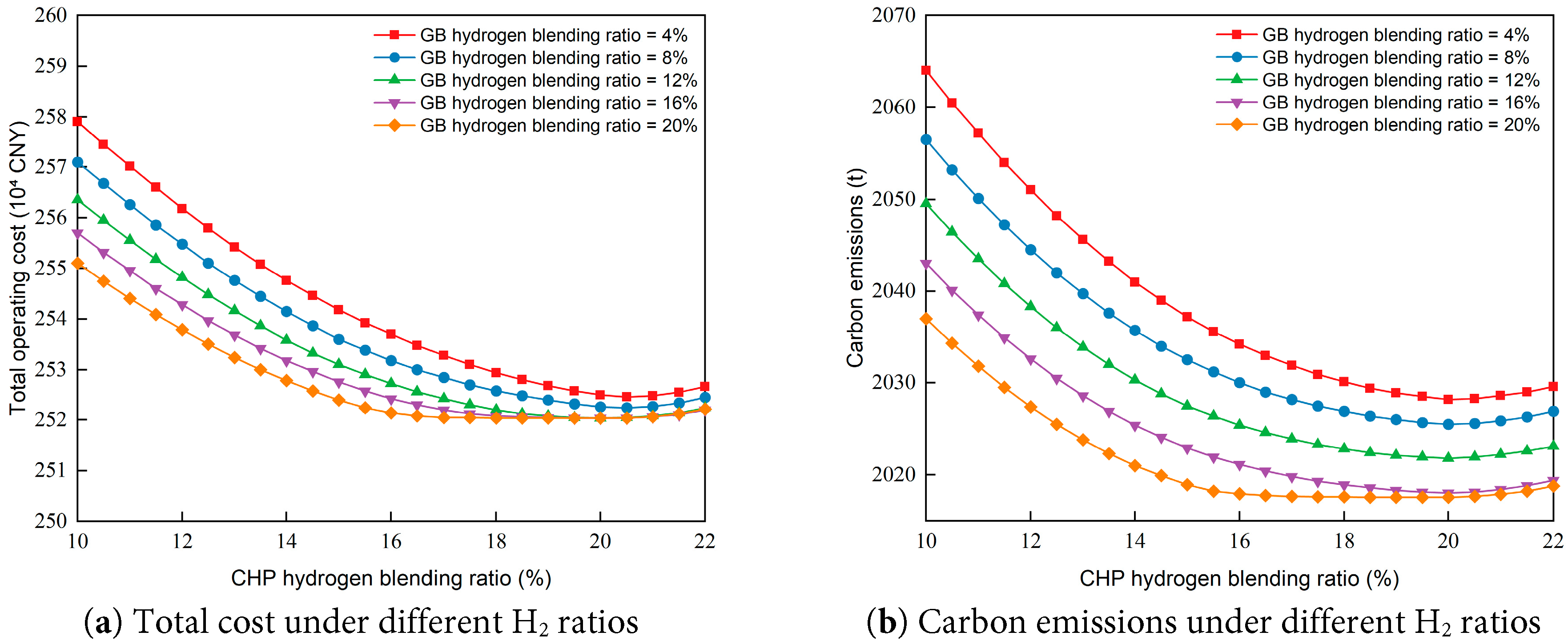
Figure 5: Variations in total system cost and carbon emissions under different hydrogen blending ratios.
Therefore, hydrogen blending can improve both the economic and low-carbon performance of the system, but a higher blending ratio does not necessarily lead to better results. For the case studied in this paper, the system achieves the best overall performance in terms of both total cost and carbon emissions when the hydrogen blending ratio of the CHP is 20%. Based on the above analysis, the optimal dispatch results of the proposed VPP model over a typical day are further analyzed under the hydrogen blending parameters with better overall performance, in order to reveal the coordinated operating mechanism of electricity, heat, gas, and hydrogen in the system.
5.4 Operating Results of the Proposed VPP Model
Fig. 6a presents the optimal electric power dispatch results of the VPP over a typical day. During the nighttime period from 1:00 to 5:00, photovoltaic generation is unavailable, and the electric load is mainly supplied by wind power, the CHP unit, the coal-fired unit, and the CSP plant. The CSP plant can still maintain a certain level of power output at night by utilizing the thermal energy collected during the daytime and stored in the thermal storage system, thereby enhancing the system’s intertemporal regulation capability. During this period, the electrolyzer, the CCS unit, and the energy storage system are also in operation, and their electricity demand is supplied through the coordinated dispatch of internal power sources. As photovoltaic output gradually increases during the daytime 6:00–14:00, the share of renewable energy in the power supply continues to increase. The system absorbs surplus renewable electricity by increasing the power consumption of the electrolyzer and the charging power of the energy storage system, which helps improve renewable energy utilization. After 14:00, as photovoltaic output gradually decreases, the outputs of the CHP unit and the coal-fired unit increase accordingly, while the energy storage system shifts from charging to discharging for peak regulation. During the evening peak period from 18:00 to 21:00, the CHP unit and the coal-fired unit undertake the main power supply task, while energy storage discharging and CSP generation jointly maintain the electric power balance of the system.
Fig. 6b shows the optimal thermal power dispatch results of the VPP over a typical day. During the nighttime period, the thermal load is mainly supplied by the CSP plant, the gas boiler, and the recovered waste heat from the CHP unit. During the daytime, with changes in the system operating state, the CSP plant and the thermal storage unit participate coordinately in thermal regulation, thereby reducing the heat supply burden of the gas boiler. When the thermal load increases in the evening, the CSP plant, the gas boiler, and the thermal storage unit jointly provide heat to maintain the thermal balance of the system.
Fig. 6c shows the natural gas balance of the system over a typical day. Natural gas in the system is mainly obtained from external gas purchase and methanation production, and is primarily consumed by the CHP unit and the gas boiler. With load variations, the amount of externally purchased natural gas and the gas consumption of the related equipment fluctuate accordingly. The methanation reactor converts hydrogen produced by the electrolyzer and CO2 captured by the CCS unit into synthetic natural gas. This process not only reduces the demand for external natural gas purchase, but also promotes CO2 utilization and hydrogen consumption, thereby helping lower the carbon-related cost of the system and improve its low-carbon operating performance.
Fig. 6d presents the hydrogen balance of the system over a typical day. Hydrogen is mainly produced by the electrolyzer and is used for methanation, hydrogen blending in gas-fired equipment, and combined heat and power generation through the HFC. Meanwhile, the hydrogen storage device achieves intertemporal balancing through hydrogen charging and discharging. The introduction of the hydrogen energy chain enhances the system’s cross-period energy shifting capability and improves the utilization of surplus wind and photovoltaic power.
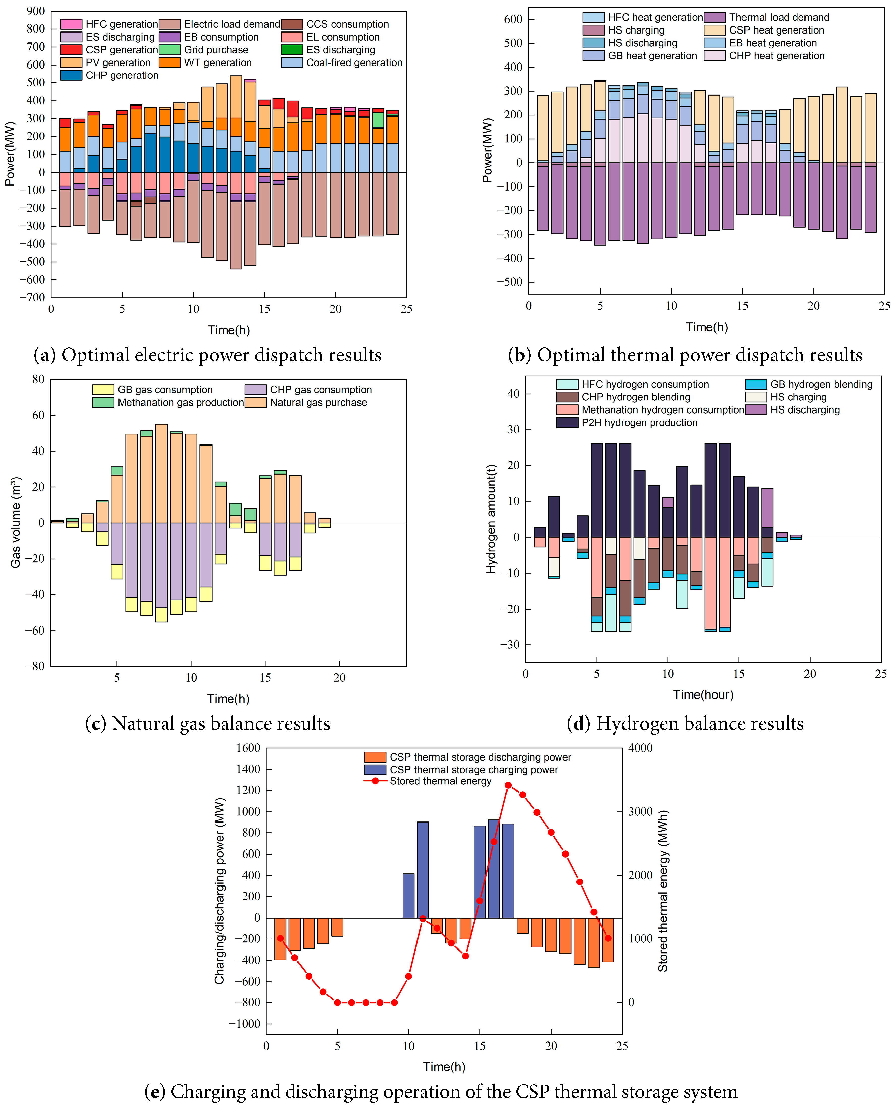
Figure 6: Multi-energy optimal dispatch results of the virtual power plant in Scenario 6.
Fig. 6e illustrates the operating state of the thermal storage system and the variation of stored thermal energy over a typical day. During the nighttime period from 1:00 to 8:00, the thermal load demand is relatively high, and the thermal storage unit continuously releases heat to participate in heat supply. As a result, the discharging power remains at a relatively high level, and the stored thermal energy gradually decreases, reaching a low level during 6:00–8:00. As the system operating state changes during the daytime, the thermal storage unit starts charging during 9:00–11:00 by storing surplus thermal energy, and the stored thermal energy gradually recovers. During 12:00–14:00, the thermal storage unit enters the discharging state again to meet the thermal load demand and maintain thermal power balance. During 15:00–17:00, the thermal energy supply is relatively sufficient, and the thermal storage unit resumes charging. The charging power reaches a relatively high level, and the stored thermal energy increases rapidly, reaching its peak at 17:00. During the evening period from 18:00 to 24:00, as the thermal load rises again, the thermal storage unit gradually releases the stored heat for heat supply regulation. Accordingly, the discharging power increases and the stored thermal energy decreases.
5.5 Comparative Analysis of the Conventional User Satisfaction Model and the Proposed Model
To verify the effectiveness of the proposed asymmetric user satisfaction model, the conventional user satisfaction model in Ref. [23] is selected as the comparison model. Under the same demand response conditions, the load adjustment results and the corresponding changes in user satisfaction under the two models are compared and analyzed.
Fig. 7 shows the demand response results of electric and thermal loads under the conventional user satisfaction model and the proposed model. It can be seen that, compared with the original load curves, both electric and thermal loads are adjusted to different extents in the two models, indicating that the established demand response model is capable of achieving a certain degree of load shifting. On this basis, after different user satisfaction models are adopted, noticeable differences can be observed in the load adjustment results during some periods. The conventional user satisfaction model treats load deviations symmetrically, whereas the proposed model takes into account users’ differentiated perceptions of load deviations in different directions. As a result, the load adjustment process can be optimized in a more targeted manner, and the demand response results are more consistent with actual user response characteristics.
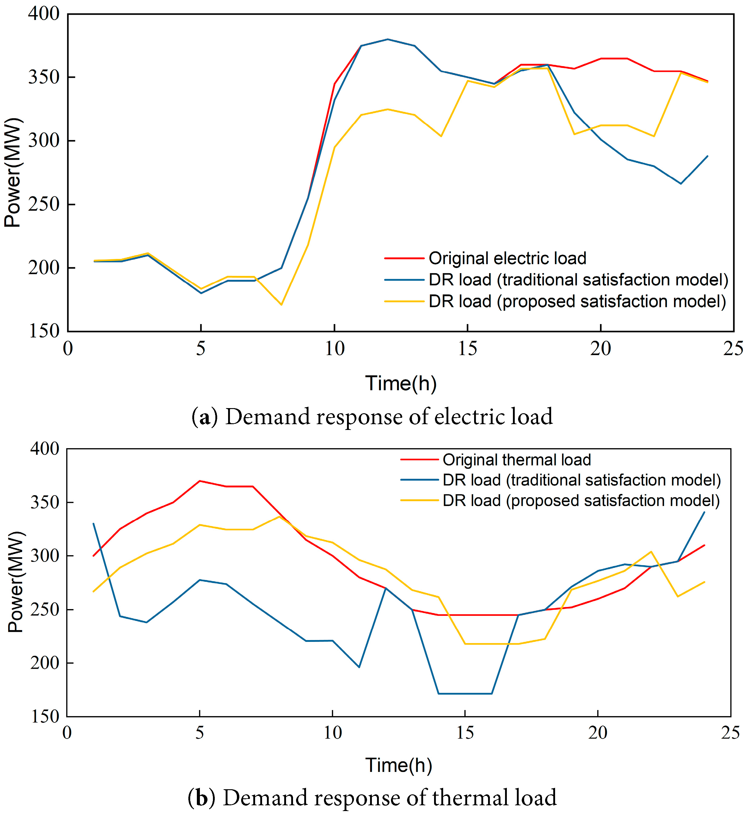
Figure 7: Comparison of electric and thermal load demand response results under different user satisfaction models.
Fig. 8 further presents the variations in user satisfaction of electric and thermal loads under the two user satisfaction models, where Fig. 8a and Fig. 8b show the temporal curves of electric load satisfaction and thermal load satisfaction, respectively. It can be seen that, under both models, user satisfaction in all periods remains above the minimum satisfaction constraint, indicating that the demand response model developed in this paper can satisfy users’ basic use requirements. On this basis, compared with the conventional user satisfaction model, the proposed asymmetric user satisfaction model maintains electric and thermal load satisfaction at a generally higher level, with relatively smaller fluctuations. In particular, during periods with more pronounced load adjustment, user satisfaction under the conventional model tends to decline more obviously, whereas the proposed model is still able to maintain a relatively high satisfaction level.
Further evidence can be found from Table 3, which shows that the average satisfaction levels of both electric and thermal loads under the proposed model are higher than those under the conventional user satisfaction model. This indicates that the proposed asymmetric user satisfaction model can more reasonably capture users’ differentiated responses to load deviations in different directions. While meeting the requirements of demand response regulation, it can effectively mitigate the adverse impact of load adjustment on users’ energy-use experience, thereby improving the rationality of demand response modeling.
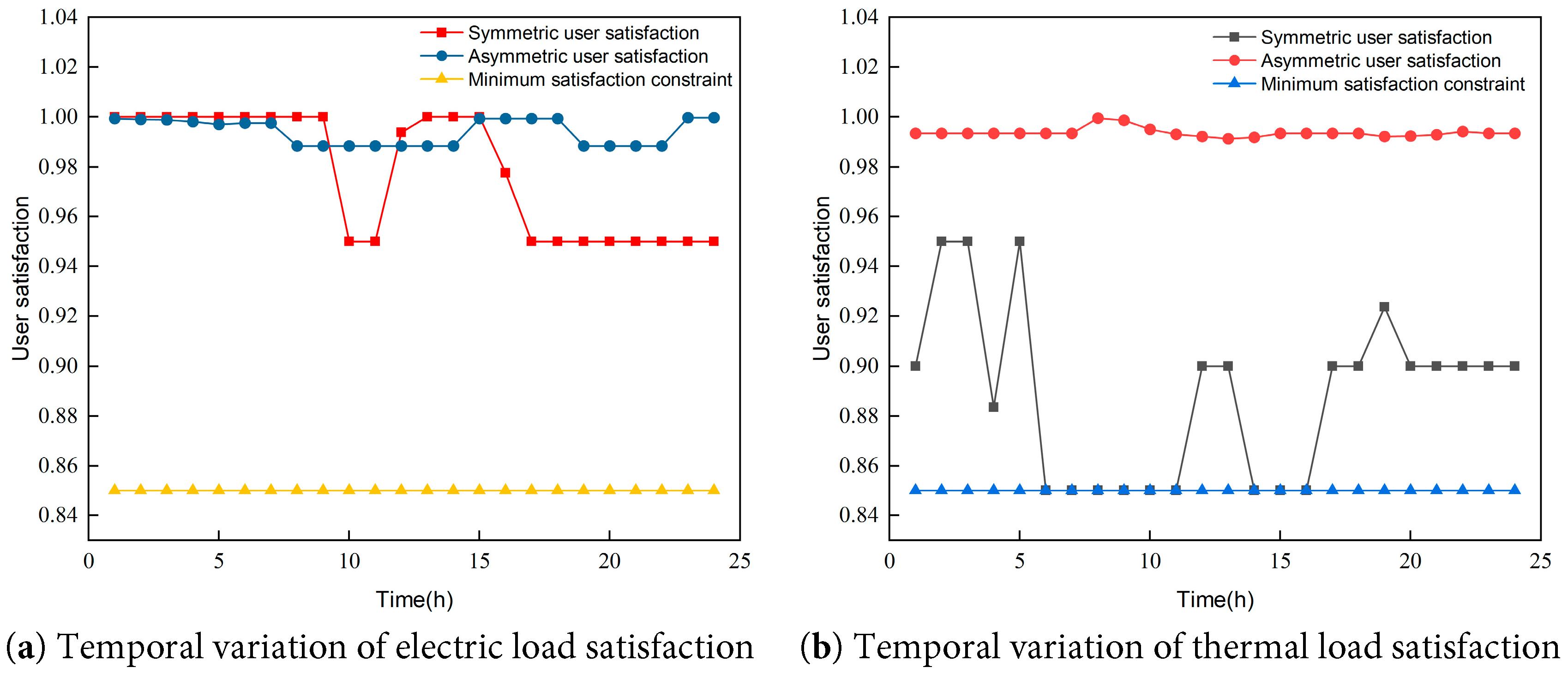
Figure 8: Temporal variations of electric and thermal load satisfaction under different user satisfaction models.
5.6 Comparative Analysis of CSP–Hydrogen Synergistic Operation
To further quantify the complementary effects of the CSP plant and the hydrogen energy system in terms of regulation timescale and energy utilization mode, this paper conducts a comparative analysis of CSP–hydrogen coordinated operation based on the relevant scenarios in Table 3. Specifically, Scenario 1 represents the traditional VPP benchmark model, Scenario 2 represents the case in which only the CSP plant is introduced, Scenario 7 represents the case in which only the complete hydrogen energy chain is introduced, and Scenario 4 represents the joint operation of the CSP plant and the hydrogen energy chain. By comparing the total operating cost, wind and photovoltaic curtailment penalty cost, carbon emissions, and gas purchase cost under these scenarios, the effects of the CSP plant, the hydrogen energy chain, and their joint configuration on the VPP operation results are analyzed.
As shown in Table 3, after the CSP plant is introduced into the traditional VPP in Scenario 2, the total system cost decreases from 5.5113 million yuan to 3.2030 million yuan, corresponding to a reduction of 41.9%. Meanwhile, the wind and photovoltaic curtailment penalty cost decreases from 0.4351 million yuan to 0.0580 million yuan. This indicates that the CSP plant can provide flexible heat supply and power regulation through its thermal storage system, thereby alleviating electricity–heat coupling constraints and effectively improving wind and photovoltaic power accommodation.
Scenario 7 represents the case in which only the complete hydrogen energy chain is introduced without the CSP plant. In this scenario, the wind and photovoltaic curtailment penalty cost decreases from 0.4351 million yuan in Scenario 1 to 0.0295 million yuan, and the electricity purchase cost is reduced to zero. This indicates that the hydrogen energy chain can absorb surplus wind and photovoltaic power through electrolytic hydrogen production and realize energy conversion and reuse through hydrogen storage, fuel cells, hydrogen blending, and methanation, thereby expanding the accommodation pathways of renewable energy. However, carbon emissions in Scenario 7 increase from 3175.03 t in Scenario 1 to 3785.02 t. The main reason is that the operation of electrolytic hydrogen production and carbon capture equipment increases the system electric load. In the absence of the intraday flexible regulation capability provided by the CSP plant, the additional electric load is mainly supplied by coal-fired units, resulting in increases in both coal-fired unit cost and carbon emissions.
When the CSP plant and the hydrogen energy chain are simultaneously introduced in Scenario 4, the total system cost further decreases to 2.7446 million yuan, and the wind and photovoltaic curtailment penalty cost is reduced to zero. Compared with Scenario 7, in which only the hydrogen energy chain is introduced, carbon emissions in Scenario 4 decrease from 3785.02 t to 2475.80 t, representing a reduction of 34.6%. Compared with Scenario 2, in which only the CSP plant is introduced, Scenario 4 shows a certain increase in carbon emissions, but the gas purchase cost is further reduced, and the wind and photovoltaic curtailment penalty cost decreases to zero. These results indicate that the joint operation of the CSP plant and the hydrogen energy chain enables a comprehensive trade-off among reducing gas purchase cost, improving renewable energy accommodation, and controlling carbon emissions.
Further analysis shows that the CSP plant and the hydrogen energy chain are complementary in terms of power regulation and energy utilization mode. The CSP plant participates in intraday electricity–heat coordination through its thermal storage system, providing short-term peak regulation and electricity–heat decoupling capability. In contrast, the hydrogen energy chain realizes the cross-period utilization of surplus wind and photovoltaic power through electrolytic hydrogen production, hydrogen storage, fuel cells, and hydrogen blending. Under their coordinated operation, the system can improve renewable energy accommodation during periods of surplus wind and photovoltaic generation and provide multi-energy complementary support during peak load periods or periods of insufficient renewable generation, thereby improving the comprehensive operational performance of the system.
Further comparison between Scenarios 5 and 6 shows that, after demand response and the user satisfaction mechanism are introduced on the basis of CSP–hydrogen coordinated operation, source–load coordinated optimization is further achieved. Compared with the symmetric satisfaction model in Scenario 5, the asymmetric user satisfaction model adopted in Scenario 6 increases the average electric load satisfaction from 0.97435 to 0.99404 and the average thermal load satisfaction from 0.88547 to 0.99361. Meanwhile, the total system cost decreases to 2.5204 million yuan, and carbon emissions decrease to 2017.54 t. These results indicate that the asymmetric user satisfaction model can further improve the comprehensive operational performance of the system while ensuring users’ energy-use experience.
Therefore, the CSP plant and the hydrogen energy chain are not simply connected to the system in parallel, but form complementary regulation capabilities within a unified optimal dispatch framework. The CSP plant mainly contributes to intraday electricity–heat coordination and short-term regulation, whereas the hydrogen energy chain mainly undertakes surplus wind and photovoltaic power conversion and cross-period energy utilization. Under the case-study conditions of this paper, their joint operation can improve renewable energy accommodation and reduce system operating cost. In the complete model, they further cooperate with demand response and the asymmetric user satisfaction mechanism to achieve coordinated optimization among economic performance, low-carbon operation, and user satisfaction.
5.7 Sensitivity Analysis of Asymmetric Satisfaction Parameters
To further analyze the influence of key parameters in the asymmetric user satisfaction model on the optimization results, the ratio of the negative to positive deviation penalty coefficients, λs = α−/α+, is selected as the sensitivity analysis parameter. Here, α+ denotes the penalty coefficient for positive load deviation, while α− denotes the penalty coefficient for negative load deviation. When λs = 1.0, the same penalty coefficient is adopted for positive and negative load deviations, and the model degenerates into the traditional symmetric satisfaction model. When λs > 1, it indicates that users are more sensitive to load curtailment or insufficient energy supply than to load increase, and the model therefore exhibits asymmetric satisfaction characteristics.
With the other parameters kept unchanged, λs is set to 1.0, 1.5, 2.0, and 2.5, respectively. The total operating cost, carbon emissions, DR and satisfaction penalty cost, average satisfaction of electric load, and average satisfaction of thermal load are compared, and the results are shown in Table 4.
As can be seen from Table 4, when λs = 1.0, the same penalty coefficient is adopted for positive and negative load deviations, and the model degenerates into the traditional symmetric satisfaction model. In this case, the average satisfaction of electric load and thermal load is 0.97435 and 0.88547, respectively, and the DR and satisfaction penalty cost is 235,348.19 yuan. This indicates that when positive and negative load deviations are treated symmetrically, the model cannot fully reflect users’ differentiated perception of load deviations in different directions, especially resulting in relatively low thermal load satisfaction.
Table 4: Sensitivity analysis results of asymmetric penalty coefficient ratio.
| Asymmetric Penalty Coefficient Ratio | Total Operating Cost | Carbon Emissions | DR & Satisfaction Cost | Avg. Electric Satisfaction | Avg. Thermal Satisfaction |
|---|---|---|---|---|---|
| 1.0 | 2,586,592.01 | 2310.26 | 235,348.19 | 0.97435 | 0.88547 |
| 1.5 | 2,548,654.05 | 2285.38 | 165,239.20 | 0.98761 | 0.96243 |
| 2.0 | 2,520,357.65 | 2017.54 | 127,871.98 | 0.99404 | 0.99361 |
| 2.5 | 2,539,874.48 | 2176.29 | 132,588.37 | 0.99520 | 0.99413 |
When λs increases from 1.0 to 2.0, the average satisfaction of electric load increases from 0.97435 to 0.99404, and the average satisfaction of thermal load increases from 0.88547 to 0.99361. Meanwhile, the DR and satisfaction penalty cost decreases from 235,348.19 yuan to 127,871.98 yuan, the total operating cost decreases from 2,586,592.01 yuan to 2,520,357.65 yuan, and carbon emissions decrease from 2310.26 t to 2017.54 t. These results indicate that an appropriate increase in the negative deviation penalty coefficient can make the model place greater emphasis on users’ sensitivity to negative load deviations, such as load curtailment, thereby improving the demand response regulation results and making load adjustment more consistent with users’ actual energy-use perception. While improving user satisfaction, the system operating cost and carbon emissions are also reduced.
When λs further increases to 2.5, the average satisfaction of electric load and thermal load increases to 0.99520 and 0.99413, respectively. However, the total operating cost increases from 2,520,357.65 yuan to 2,539,874.48 yuan, carbon emissions increase from 2017.54 t to 2176.29 t, and the DR and satisfaction penalty cost also increases from 127,871.98 yuan to 132,588.37 yuan. This indicates that an excessively large negative deviation penalty coefficient strengthens the user satisfaction constraint, compresses the feasible space for load regulation, and consequently weakens the optimization effect of demand response on system economy and low-carbon performance.
Therefore, the asymmetric satisfaction parameter is not necessarily better when it is larger. Instead, there exists a trade-off among economic performance, low-carbon performance, and user satisfaction.
Overall, when λs = 2.0, the system achieves the best comprehensive performance in terms of total operating cost, carbon emissions, DR and satisfaction penalty cost, and average satisfaction of electric and thermal loads. This result demonstrates that the parameter setting of the asymmetric satisfaction model adopted in this paper can effectively balance user-side energy-use experience and the low-carbon economic operation requirements of the system, thereby verifying the rationality of the proposed asymmetric user satisfaction model parameters.
In this paper, an optimal dispatch model for a CSP-hydrogen coordinated virtual power plant considering asymmetric user satisfaction is established. Based on the integrated consideration of the operational constraints of the CSP plant, hydrogen energy system, carbon capture, and demand response, the model is optimized with the objective of minimizing the total operating cost of the system. The case study results show that the proposed model can simultaneously take into account the economy, low-carbon performance, and user satisfaction of the virtual power plant. The main conclusions are as follows:
- (1)The CSP plant and the hydrogen energy system exhibit good complementarity in terms of regulation timescale and energy utilization mode. The CSP plant mainly undertakes intra-day electricity–heat coordination and short-term regulation, while the hydrogen energy system mainly provides inter-temporal energy transfer. Their coordinated operation within a unified optimal dispatch framework enhances the multi-energy regulation capability of the system and helps improve operating economy under the case-study conditions of this paper.
- (2)The coordinated operation of CSP and hydrogen energy helps improve the accommodation of wind and photovoltaic power, and reduces wind and photovoltaic curtailment as well as external energy purchase demand. Meanwhile, the carbon capture and methanation processes promote carbon dioxide utilization, reduce the system’s carbon emission pressure and carbon trading cost, and improve the low-carbon operating performance of the virtual power plant.
- (3)The proposed asymmetric user satisfaction model can better reflect users’ differentiated perceptions of load regulation in different directions. Compared with the conventional satisfaction model, the proposed model achieves more reasonable load adjustment while satisfying user satisfaction constraints, and further improves the level of user satisfaction.
Acknowledgement:
Funding Statement: This work was supported by the Natural Science Foundation of Xinjiang Uygur Autonomous Region (2023D01C187), the Tianshan Innovation Team Program of Xinjiang Uygur Autonomous Region for the Innovation Team on Basic Theory and Key Technologies of New Energy Power Systems (2025D14009), and the “Tianchi Talent” Introduction Program of Xinjiang Uygur Autonomous Region.
Author Contributions: The authors confirm contribution to the paper as follows: study conception and design, data collection, model development, simulation, analysis and interpretation of results, and draft manuscript preparation: Longwei Ma; supervision and manuscript revision: Yue Meng; review and editing: Xinkai Li, Cong Wang, and Ping Ma. All authors reviewed and approved the final version of the manuscript.
Availability of Data and Materials: The authors confirm that the data supporting the findings of this paper are available within the article.
Ethics Approval: Not applicable.
Conflicts of Interest: The authors declare no conflicts of interest.
Abbreviations
| VPP | Virtual power plant |
| WT | Wind turbine |
| PV | Photovoltaic |
| CSP | Concentrated solar power |
| CCS | Carbon capture and storage |
| CHP | Combined heat and power |
| HFC | Hydrogen fuel cell |
| EB | Electric boiler |
| GB | Gas boiler |
| EL | Electrolyzer |
| MR | Methanation reactor |
| ES | Electrical energy storage |
| HS | Heat storage tank |
| P2G | Power-to-gas |
References
1. Ren D , Xiao J , Hou J , Du E , Jin C , Liu Y . Construction and evolution of China’s new power system under dual carbon goal. Power Syst Technol. 2022; 46( 10): 3831– 9. [Google Scholar]
2. Sun Q , Jia Y , Wang Y . From virtual power plant to real electricity: summary and prospect of virtual power plant research. Power Gener Technol. 2023; 44( 5): 583– 601. [Google Scholar]
3. Peng D , Shui J , Wang D , Zhao H . Review of virtual power plant under the background of “dual carbon”. Power Gener Technol. 2023; 44( 5): 602– 15. [Google Scholar]
4. Ni Q , Xu C , Cai Z , Zhou Y , Lai LL . Optimal dispatch of integrated energy system with CCUS-P2G coupling and hydrogen-doped gas equipment based on ladder-type carbon trading mechanism. Energy. 2025; 336: 138397. doi:10.1016/j.energy.2025.138397. [Google Scholar] [CrossRef]
5. Li H , Lu X , Zhou K , Shao Z . Distributionally robust optimal dispatching method for integrated energy system with concentrating solar power plant. Renew Energy. 2024; 229: 120792. doi:10.1016/j.renene.2024.120792. [Google Scholar] [CrossRef]
6. Wei X , Xu Y , Sun H , Bai X , Chang X , Xue Y . Day-ahead optimal dispatch of a virtual power plant in the joint energy-reserve-carbon market. Appl Energy. 2024; 356: 122459. doi:10.1016/j.apenergy.2023.122459. [Google Scholar] [CrossRef]
7. Ma C , Hu Z . Low-carbon economic scheduling of integrated energy system considering flexible supply–demand response and diversified utilization of hydrogen. Sustainability. 2025; 17( 4): 1749. doi:10.3390/su17041749. [Google Scholar] [CrossRef]
8. Li Q , Zhou Y , Wei F , Li S , Wang Z , Li J , et al. Multi-time scale scheduling for virtual power plants: integrating the flexibility of power generation and multi-user loads while considering the capacity degradation of energy storage systems. Appl Energy. 2024; 362: 122980. doi:10.1016/j.apenergy.2024.122980. [Google Scholar] [CrossRef]
9. Li Y , Han M , Shahidehpour M , Li J , Long C . Data-driven distributionally robust scheduling of community integrated energy systems with uncertain renewable generations considering integrated demand response. Appl Energy. 2023; 335: 120749. doi:10.1016/j.apenergy.2023.120749. [Google Scholar] [CrossRef]
10. Lu Q , Guo Q , Zeng W . Optimization scheduling of integrated energy service system in community: A bi-layer optimization model considering multi-energy demand response and user satisfaction. Energy. 2022; 252: 124063. doi:10.1016/j.energy.2022.124063. [Google Scholar] [CrossRef]
11. Wu Q , Li C , Bai J . Optimal bidding strategy for multi-energy virtual power plant participating in coupled energy, frequency regulation and carbon trading markets. Int J Hydrogen Energy. 2024; 73: 430– 42. doi:10.1016/j.ijhydene.2024.06.067. [Google Scholar] [CrossRef]
12. Good N . Using behavioural economic theory in modelling of demand response. Appl Energy. 2019; 239: 107– 16. doi:10.1016/j.apenergy.2019.01.158. [Google Scholar] [CrossRef]
13. Kahneman D , Tversky A . Prospect theory: an analysis of decision under risk. In: Handbook of the fundamentals of financial decision making: part I. Singapore: World Scientific; 2013. p. 99– 127. [Google Scholar]
14. Duan J , Tian Q , Liu F , Xia Y , Gao Q . Optimal scheduling strategy with integrated demand response based on stepped incentive mechanism for integrated electricity-gas energy system. Energy. 2024; 313: 133689. doi:10.1016/j.energy.2024.133689. [Google Scholar] [CrossRef]
15. Duan X , Cheng Z , Zhang D , Duan X . Optimal scheduling of an integrated energy system considering demand response and two-stage P2G. J Syst Simul. 2025; 37( 8): 2139– 51. [Google Scholar]
16. Tian L , Zhu C , Deng T . Day-ahead scheduling of SMR integrated energy system considering heat-electric-cold demand coupling response characteristics. Energy Rep. 2022; 8: 13302– 19. doi:10.1016/j.egyr.2022.10.005. [Google Scholar] [CrossRef]
17. Zhou K , Peng N , Yin H , Hu R . Urban virtual power plant operation optimization with incentive-based demand response. Energy. 2023; 282: 128700. doi:10.1016/j.energy.2023.128700. [Google Scholar] [CrossRef]
18. Shi L , Liang C , Zhou J , Li Y , Liu J , Wu F . Optimal scheduling of integrated energy systems with a ladder-type carbon trading mechanism and demand response. Front Energy Res. 2024; 12: 1363285. doi:10.3389/fenrg.2024.1363285. [Google Scholar] [CrossRef]
19. Dong Y , Han Z , Li X , Ma S , Gao F , Li W . Joint optimal scheduling of renewable energy regional power grid with energy storage system and concentrated solar power plant. Front Energy Res. 2022; 10: 941074. doi:10.3389/fenrg.2022.941074. [Google Scholar] [CrossRef]
20. Cui M , Qiao X , Lu G , Yang S , Wang Y , Yang B . Consideration of low-carbon dispatching of electrothermal systems for ultra-supercritical power plants with carbon capture. In: Proceedings of the 2024 Second International Conference on Cyber-Energy Systems and Intelligent Energy (ICCSIE); 2024 May 17–19; Shenyang, China. New York, NY, USA: IEEE; 2024. p. 1– 6. [Google Scholar]
21. Chen D , Liu F , Liu S . Optimization of virtual power plant scheduling coupling with P2G-CCS and doped with gas hydrogen based on stepped carbon trading. Power Syst Technol. 2022; 46( 6): 2042– 54. [Google Scholar]
22. Chen J , Hu Z , Chen Y , Chen J , Chen W , Gao M , et al. Thermoelectric optimization of integrated energy system considering ladder-type carbon trading mechanism and electric hydrogen production. Electr Power Autom Equip. 2021; 41( 9): 48– 55. [Google Scholar]
23. Wang L , Liu X , Li Y , Chang D , Ren X . Low-carbon optimal dispatch of integrated energy system considering demand response under the tiered carbon trading mechanism. arXiv:2310.03056. 2023. [Google Scholar]
Cite This Article
 Copyright © 2026 The Author(s). Published by Tech Science Press.
This work is licensed under a Creative Commons Attribution 4.0 International License , which permits unrestricted use, distribution, and reproduction in any medium, provided the original work is properly cited.
 Downloads
 Citation Tools
