Stochastic Differential Equation-Based Dynamic Imperfect Maintenance Strategy for Wind Turbine Systems

1  Introduction

As a clean and sustainable renewable energy source, wind power has become a pillar industry in China’s new energy sector. However, the increasing structural and functional complexity of wind turbines, coupled with their unique installation sites and operational environments, has led to significantly elevated maintenance costs [1–3]. Traditional post-failure maintenance, characterized by passive response patterns and high-cost limitations, can no longer meet modern wind power operation and maintenance demands. Preventive maintenance, which reduces equipment failure probability and decreases downtime losses, has been widely adopted in engineering practice [4–6]. Preventive maintenance encompasses two primary methodologies: time-based maintenance (TBM) and condition-based maintenance (CBM). TBM constitutes scheduled maintenance interventions executed according to predetermined temporal intervals, whereas CBM involves continuous monitoring of equipment parameters, with maintenance actions triggered when operational conditions fall below established threshold values [7–9].

In existing research on preventive maintenance for wind turbines, several significant achievements have been realized. Byon et al. developed a condition-based maintenance strategy utilizing Markov properties, which enables the formulation of adaptive maintenance protocols based on real-time component status [10]. Wu et al. based on proportional hazard models, this study comprehensively incorporates diverse maintenance strategies while systematically examining their synergistic implementation mechanisms within maintenance decision-making frameworks. Employing multi-attribute decision theory, three critical performance indicators—maintenance cost rate, reliability, and availability—are optimally integrated to formulate a unified objective function. Through the development of a bi-level optimization algorithm, dynamic maintenance threshold function curves are ultimately derived upon establishing the weighting coefficients for each objective function [11,12]. Liu et al. developed a condition-based maintenance model for repairable systems subject to dependent failure processes, encompassing soft failures induced by system degradation and hard failures caused by random shocks. The model demonstrates excellent compatibility while incorporating the adverse or beneficial maintenance effects resulting from inspection, preventive maintenance, and corrective maintenance activities [13]. Li et al., based on real-time operational data of high-speed train gearboxes, developed a Weibull proportional hazard model to assess reliability, integrated entropy weighting and whitening weight functions to quantify maintainability, employed fuzzy analytic hierarchy process for safety evaluation, and constructed a multidimensional RAMS (Reliability, Availability, Maintainability, Safety) assessment framework for high-speed train gearboxes. The validity of this methodology in optimizing preventive maintenance cycles has been empirically verified [14,15]. Yu et al. employed the Cox proportional hazards model to integrate real-time degradation of critical wind turbine components, maintenance costs, power generation losses, and monitoring data into a dynamically updatable preventive maintenance scheduling framework [16]. El-Naggar et al. have proposed a phased decision-making framework predicated upon large-scale field failure-maintenance databases, with the objective of aligning the optimal maintenance strategies with each subsystem of wind turbines [17]. However, most of these studies assume that equipment can be fully restored to its initial state post-maintenance, neglecting the common occurrence of imperfect repairs in practical scenarios. Additionally, existing research inadequately characterizes the stochastic disturbances encountered during wind turbine operation, limiting the models’ ability to accurately fit the actual degradation trajectories. Fei Siqi et al. addressed the over-maintenance and under-maintenance issues of distributed energy supply equipment by proposing a preventive maintenance strategy based on an improved entropy-weighted hierarchical method [18]; however, their approach failed to explicitly incorporate reliability constraints and inadequately considered the accelerating degradation trends of equipment. Li et al. have achieved notable progress in reliability-based maintenance interval optimization research [19,20]; however, their preventive replacement initiation criteria are constrained to component replacement at the conclusion of the final preventive maintenance cycle and post-failure replacement. Lin et al. developed a preventive maintenance model utilizing boundary strength processes to characterize wind turbine component degradation. While ensuring reliability constraints, their iterative algorithm dynamically determines optimal PM intervals and frequencies to minimize operational costs per unit time [21]. However, their approach lacks an analytical methodology for reliability threshold-driven dynamic maintenance scheduling, instead relying on algorithmic optimization procedures. Yi et al. established a multi-objective optimization model using RAMS metrics as the primary framework, incorporating age-degradation and failure rate escalation factors to determine reliability thresholds and maintenance strategies following fourth-level overhauls [22]. However, their approach failed to provide analytical solutions for reliability threshold-driven non-periodic maintenance intervals and did not achieve a unified framework for component-level imperfect repair coordination with system-level techno-economic reliability optimization. Zhang et al. developed health indicators that maintain comparability under variable rotational speeds through rotational speed slicing and deviation compensation, but their work remained limited to condition assessment without establishing degradation models incorporating stochastic disturbances, integrating imperfect maintenance mechanisms, or embedding reliability-cost collaborative optimization frameworks, thus failing to address the fundamental issues of dynamic maintenance decision-making and lifecycle economic optimization [23]. Szubartowski et al. developed a semi-Markov preventive maintenance model for the Enercon E82-2 wind turbine, optimizing maintenance intervals using profitability and asymptotic availability as performance metrics [24]; however, their framework implicitly assumes “as-good-as-new” restoration and piecewise constant failure rates, failing to characterize nonlinear degradation trajectories driven by stochastic perturbations, neglecting to incorporate imperfect maintenance mechanisms such as age reduction and increasing failure rates, and omitting reliability thresholds from dynamic interval optimization and life-cycle cost trade-offs, thereby presenting limitations in accelerated degradation scenarios and integrated economic-reliability decision-making.

To address the aforementioned bottlenecks, this paper proposes a dynamic imperfect maintenance strategy incorporating reliability constraints based on stochastic differential equations (SDE). The core contributions are manifested in: 1. At the degradation modeling level, Brownian motion terms and state-dependent rate functions are introduced, explicitly coupling stochastic perturbations into the failure processes of critical wind turbine components for the first time. Compared to conventional ODE/semi-Markov frameworks, residuals are reduced by 16%, significantly enhancing trajectory fitting accuracy; 2. At the maintenance mechanism level, age reduction factors and failure rate increase factors are integrated, transcending the “as-good-as-new” assumption to characterize the engineering reality of “post-maintenance condition between new and old states,” making the strategy more aligned with the technical boundaries of irreversible damage accumulation; 3. At the decision optimization level, reliability thresholds Rp and Rr serve as dual-driving parameters to establish analytical formulas for dynamic maintenance intervals, incorporating replacement, imperfect maintenance, minimal repair, and downtime losses into the life-cycle cost function to achieve synergistic optimization of reliability and economics. Validation using gearbox data from Jiuquan Wind Farm demonstrates that compared to conventional fixed-interval strategies, the optimized TBIM extends service life by 4.4% and reduces average maintenance costs by 4.16% at Rp = 0.8; under high-reliability scenarios at Rp = 0.9, life extension reaches 17.2% with cost reduction of 14.6%. In summary, the proposed model provides an integrated solution of “precise degradation characterization-imperfect repair modeling-reliability-economic synergistic optimization” for wind turbine preventive maintenance, effectively addressing systematic deficiencies in existing research regarding stochastic perturbation representation, imperfect repair characterization, and dynamic decision analytics.

2  Degradation Model of Wind Turbine Equipment Condition

2.1 Construction of the Stochastic Differential Equation (SDE)

In constructing a condition degradation model for wind turbine equipment, and acknowledging the stochastic disturbances from external forces, this paper develops a state degradation model based on stochastic differential equations. Prior to modeling, the following definitions and assumptions are specified.

Definitions:

Definition 1: x(t) represents the state of the equipment at time t, with changes in x(t) signifying the evolution of the equipment’s condition throughout its lifecycle. Specifically, x(t) = 1 indicates the equipment is in a brand-new state, while x(t) = 0 denotes a completely failed state.

Definition 2: The failure rate of equipment is influenced by both its operational state and service time, where the impact of stochastic interventions (e.g., inspections, maintenance) is state-dependent.

Assumptions:

Assumption 1: The stochastic disturbances affecting the equipment at different times are independent and identically distributed, with an expected value of zero.

Assumption 2: Equipment maintenance can be completed instantaneously, with each maintenance event initiating a new operational lifecycle for the equipment. The function x(t) characterizes the state evolution process of the equipment throughout a single lifecycle period.

Assumption 3: Both TBM and CBM are replacement maintenance strategies, where the component is restored to an as-new condition post-replacement, effectively resetting the failure rate to zero.

Based on the aforementioned definitions and assumptions, the state degradation model for wind turbine equipment constructed using stochastic differential equations is presented in Eq. (1):

dx(t)=−λ(x(t),t)dt+u(x(t),t)dB(t)(1)

where λ(x(t), t) denoting the failure rate; u(x(t), t) is the stochastic perturbation coefficient; and B(t) is a Brownian motion, consistent with Assumption 1.

The aforementioned SDE degradation model comprises two components: −λ(x(t), t) characterizes intrinsic equipment deterioration (such as gearbox wear), while u(x(t), t)dB(t) quantifies stochastic perturbations (including inspection and maintenance activities), thereby addressing the limitation of conventional models that neglect environmental stochasticity.

Let λ(x(t), t) and u(x(t), t) be measurable functions defined on the domain of interest. There exists a constant K that satisfies Eqs. (2) and (3):

|λ(x(t),t)−λ(y(t),t)|+|μ(x(t),t)−μ(y(t),t)|≤K|x(t)−y(t)|(2)

|λ(x(t),t)|+|μ(x(t),t)|≤K(1+|x(t)|)(3)

where x(t) and y(t) represent the solutions to Eqs. (1)–(3) serve to establish the existence and uniqueness of the solution to Eq. (1). If both Eqs. (2) and (3) are satisfied, then Eq. (1) possesses a unique solution x(t), and this unique solution is continuous with respect to t [25].

2.2 Construction and Comparison of Condition-Based Maintenance (CBM) and Time-Based Maintenance (TBM) Models

Building upon the stochastic differential equation (SDE) framework established in the preceding section, this section proceeds from the macroscopic SDE degradation model as a foundation to develop refined condition-based maintenance (CBM) and time-based maintenance (TBM) models. Subsequently, leveraging the distinct characteristics of CBM and TBM approaches, corresponding state deterioration models are formulated, with comprehensive analysis of their intrinsic relationships and interdependencies.

2.2.1 Development of Degradation Models for Condition-Based Maintenance (CBM)

Condition-based maintenance (CBM) is a maintenance strategy that relies on real-time monitoring of equipment condition to trigger maintenance actions when the condition falls below a predefined preventive maintenance threshold, necessitating thorough consideration of the equipment’s condition data.

In this paper, the failure rate of equipment is conceptualized as comprising two components: the intrinsic failure rate and the state-dependent influence rate. The intrinsic failure rate represents the fundamental degradation process influenced by time, typically determined by the equipment’s lifetime distribution model. Among the prevailing lifetime distribution models, the Weibull distribution is particularly suitable due to its flexible shape and scale parameters, which allow it to accurately characterize failure rates that increase, decrease, or remain constant over time. This adaptability aligns well with the lifetime distributions of mechanical components in complex equipment. Extensive engineering practice has further demonstrated that the lifetime data of rotating machinery operating under complex load conditions, such as wind turbines, often exhibit typical Weibull characteristics. Therefore, this study adopts the Weibull distribution to model the intrinsic failure rate, as shown in Eq. (4):

h(t)=βη(tη)β−1(4)

where β is the shape parameter,determines the form of h(t); and η is the scale parameter, Determined the peak value and amplitude of h(t);. The specific effects of varying β and η on h(t) are illustrated in Figs. 1 and 2.

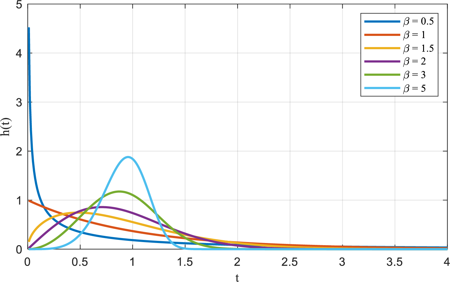
Figure 1: Images of h(t) under different η

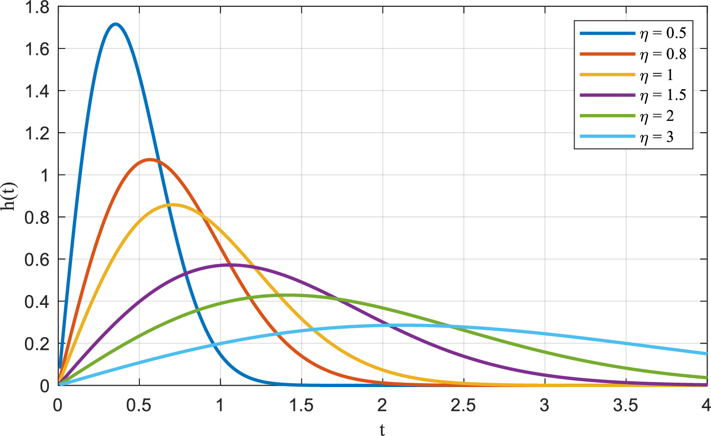
Figure 2: Images of h(t) under different η

As illustrated in Figs. 1 and 2, the Weibull distribution exhibits pronounced sensitivity to parameter variations, with the shape parameter β exerting a particularly significant influence. Depending on the value of β, the distribution can assume the form of several classical distributions: when β equals 1, it mirrors the characteristics of the exponential distribution; when β is 2, it approximates the Rayleigh distribution; and when β ranges from 3 to 4, its curve closely aligns with the normal distribution.

These observations underscore that, by accurately estimating the shape and scale parameters, the Weibull distribution can precisely characterize the lifetime behavior of wind turbine components. It is important to note that the applicability of this approach extends beyond the wind power sector; the Weibull model can effectively represent the life patterns of other complex, large-scale industrial components as well. Consequently, the model presented in this study is equally suitable for the state modeling of other major equipment.

The state influence rate, denoted as g(x(t)), accounts for the increase or decrease in the base failure rate due to the equipment’s condition. Assuming g(x(t)) is a continuous function with a domain of [0, 1], according to Weierstrass’s first approximation theorem, it is possible to construct a polynomial p(x(t))=a0+a1⋅x(t)+a2⋅x(t)2+⋯+an−1⋅x(t)n−1+an⋅x(t)n that uniformly approximates g(x(t)) arbitrarily closely. For any given polynomial p(x(t)), regardless of the value of x(t), there always exists an adjustable coefficient k such that q(x(t)) approaching p(x(t)), it can thus be considered that q(x(t)) asymptotically converges to g(x(t)).

q(x(t))=a0+ε⋅x(t)+(ε⋅x(t))2+⋯+(ε⋅x(t))k−1+(ε⋅x(t))k(5)

When x(t) = 0, the equipment has completely failed and no longer contributes to subsequent failure rates. Therefore, g(0) = 1, which leads to q(0) = a0 = 1. Consequently, q(x(t)) can be expressed as:

q(x(t))=1+ε⋅x(t)+(ε⋅x(t))2+⋯+(ε⋅x(t))k−1+(ε⋅x(t))k(6)

As indicated by Eq. (6), the expansion of q(x(t)) aligns with the Taylor series of g(x(t)), thus the expression for g(x(t)) can be represented as shown in Eq. (7):

g(x(t))=11−ε⋅x(t)(7)

where ε represents the parameter quantifying the impact of the equipment’s condition on the baseline failure rate, also known as the regression coefficient.

From Eqs. (4) and (7), the failure rate function is obtained as shown in Eq. (8):

λ(x(t),t)=βη(tη)β−1⋅11−ε⋅x(t)(8)

The stochastic disturbance in Eq. (1) is independent of time and space, depending only on the current operational state of the equipment; therefore, u(x(t), t) can be expressed as Eq. (9):

u(x(t),t)=k⋅x(t),(9)

where k denotes the stochastic perturbation parameter.

Substituting Eqs. (8) and (9) into Eq. (1), the condition-based maintenance (CBM) degradation model is formulated as Eq. (10):

dx(t)=−βη(tη)β−1⋅11−ε⋅x(t)⋅dt+k⋅x(t)dB(t)(10)

From an engineering perspective, the maintenance principle of CBM is to carry out maintenance when the state value of the equipment is lower than the preventive maintenance threshold. That is, let the preventive maintenance threshold be Xth, when the state value is less than Xth at a certain moment τ, the repair is carried out immediately, then τ should satisfy Eqs. (11) and (12).

x(τ)≤Xth,(11)

τ=inf{t>0;x(t)≤Xth<1}.(12)

It should be noted that this model explicitly defines only the preventive maintenance threshold Xth, without introducing an independent functional failure threshold. The primary reasons are as follows:

(1)   The lower bound of the state variable x(t) ∈ [0, 1], namely x = 0, is designated as an absorbing state. Once the trajectory reaches this boundary, it is regarded as a functional failure, triggering corrective replacement. Mathematically, this is equivalent to the “functional failure threshold” in conventional dual-threshold models;

(2)   Within the stochastic degradation framework, imposing a fixed hard threshold Xf ∈ (0, 1) leads to excessive variance in the first passage time, thereby undermining the robustness of decision-making;

(3)   In subsequent sections, this study dynamically quantifies failure risk using reliability thresholds Rp and Rr, which also provide a robust buffer for monitoring errors, making it unnecessary to explicitly introduce Xf.

However, the CBM model developed in this study incorporates a stochastic disturbance term, resulting in a component degradation process that no longer follows a single deterministic trajectory. The corresponding maintenance schematic is illustrated in Fig. 3.

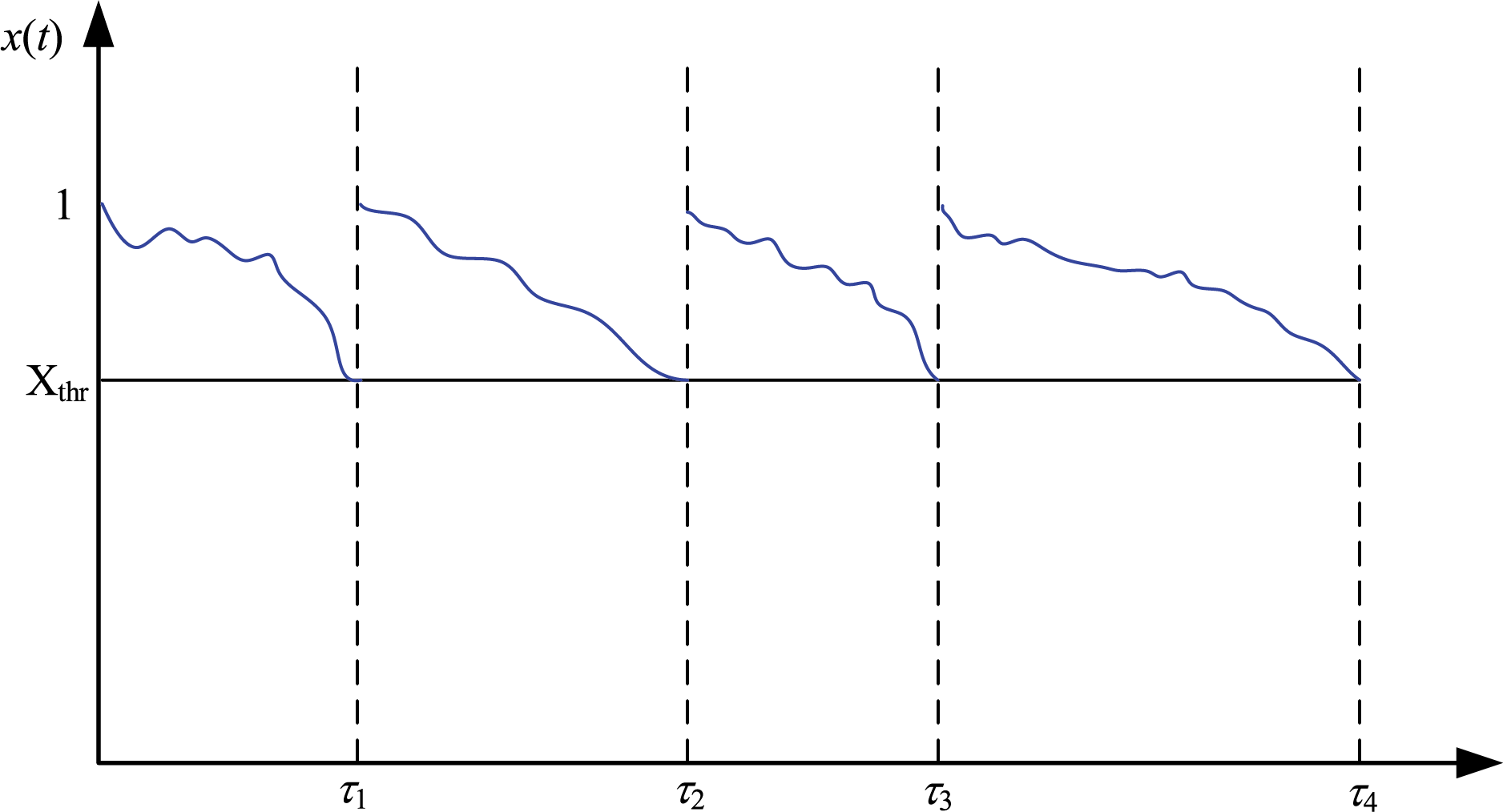
Figure 3: The principles of Condition-Based Maintenance (CBM)

As illustrated in Fig. 3, Condition-Based Maintenance (CBM) models primarily monitor the critical states of a system, initiating preventive maintenance upon breach of a predefined maintenance threshold. However, the inherent stochasticity in system states introduces unpredictability, thereby precluding precise forecasting of CBM implementation times. This uncertainty can lead to untimely or inadequate maintenance actions, resulting in equipment under-maintenance.

2.2.2 Development of Degradation Models for Condition-Based Maintenance (CBM)

In time-based maintenance (TBM), equipment is periodically maintained at predetermined intervals, as illustrated in Fig. 4. Consequently, the state function of a TBM model can be regarded as a fixed trajectory. Mathematically, the TBM model represents the expectation of the condition-based maintenance (CBM) model, where TBM is the average state trajectory of all CBM model state sample paths [25].

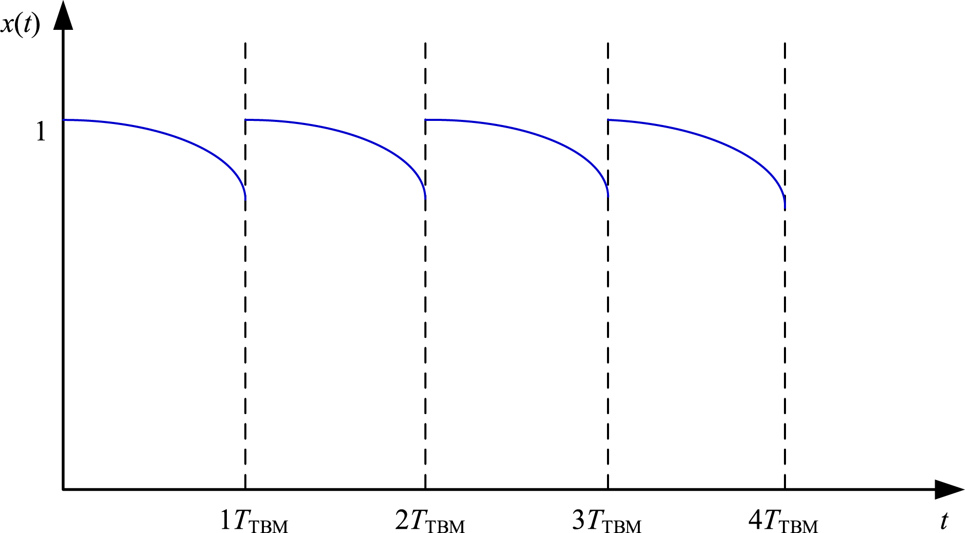
Figure 4: The principles of Time-Based Maintenance (TBM)

Based on assumption (1), the expected value of the stochastic disturbance is zero, causing the TBM degradation model to degenerate from a stochastic differential equation (SDE) to the ordinary differential equation presented in Eq. (13).

dx(t)=−λax(t)dt(13)

where lax(t) denotes the mean failure rate within the Condition-Based Maintenance (CBM) degradation model.

The function lax(t) represents the expected value of failure rates across various CBM samples, aiming to characterize the failure rate within the TBM degradation model by averaging the failure rates from all CBM degradation model trajectories. Current monitoring technologies and data transmission speeds are sufficient to ensure accurate information transfer between the CBM and TBM models.

At time t, the condition-based maintenance (CBM) sample path for a device is represented by x(wi, t), where i = 1, 2, …, n. Consequently, the historical data acquired from the Supervisory Control and Data Acquisition (SCADA) system yields lax(t), as expressed in Eq. (14).

λa(t)=E[1n∑i=1n1x(ωi,t)+1N∑i=1N1τi]=1n∑i=1n1Ex(ωi,t)+1N∑i=1N1τi(14)

By comparing Eqs. (10) and (13), it can be observed that the TBM degradation model averages the stochastic perturbations, resulting in a smoothed trajectory. This smoothed trajectory represents the mean of the CBM model’s trajectories in the presence of stochastic perturbations. When a sufficiently large number of sample trajectories are considered, the expectation of the CBM can be regarded as the TBM. It should be noted that while the failure rate lax(t) in the TBM degradation model is derived through statistical averaging of historical condition monitoring data from CBM, it operates independently of real-time condition monitoring during field implementation.

From the preceding analysis, it is inferred that as the sample path approaches infinity, the asymptotic relationship between TBM and CBM can be expressed as shown in Eq. (15).

x∗(TTBM)=Xth=x(τi)(15)

where x∗ represents the equipment’s condition at the TBM maintenance threshold.

From Eq. (15), it is evident that during TBM maintenance execution, the equipment condition x∗(TTBM) approaches the preventive maintenance threshold Xth established in the CBM model. Concurrently, this demonstrates that the equipment condition also approaches Xth upon reaching the CBM shutdown point. This indicates that equipment failures predominantly occur in proximity to TBM maintenance intervals, thereby validating the efficacy of the TBM model. therefore, core maintenance resources should be pre-positioned near these TBM time points. Alternative failure modes necessitate reliance on emergency repair mechanisms or the implementation of unconventional rapid replacement procedures for resolution.

2.3 Model Parameter Estimation and Validation Are Performed

2.3.1 Model Parameter Estimation Is Performed

1.   The failure rate parameter

From Eq. (8), the reliability function of the model is obtained as expressed in Eq. (16):

R(x(t),t)=exp⁡[−∫0tλ(x(t),t)dt]=exp⁡[−(tη)β11+ε⋅x(t)](16)

The likelihood function is constructed from the failure probability density function f(x(t),t)=λ(x(t),t)×R(x(t),t), as presented in Eq. (17).

L(β,η,ε)=∏i=1rβη(tiη)β−1⋅ε1+ε⋅x(ti)⋅∏i=1Nexp⁡[−(tiη)βε1+ε⋅x(ti)](17)

where N represents the total number of monitored data points; r denotes the count of fault data points within N, and x(ti) signifies the data detection value at time ti.

By taking the logarithm of both sides of Eq. (17) and simplifying, Eq. (18) is obtained:

ln⁡L(β,η,ε)=rln⁡βη+∑i=1n[(β−1)ln⁡(tiη)−ln⁡(1+εx(ti))]−∑j=1N[(tiη)β11+ε⋅x(ti)](18)

The parameters η, β, and ε of the failure rate model are solved using the Newton-Raphson iterative method [26].

2.   Stochastic perturbation parameter

To ascertain the stochastic perturbation parameter k, the stochastic differential equation is subjected to discretization and statistical analysis. Initially, the time interval (0, T) is discretized into tn = nΔt(n = 0, 1, …, N) using a step size of Δt. Over the interval Δt, the variation in the state value, denoted as Δxn(t), is recorded as shown in Eq. (19).

Δxn(t)=∫0Δtλ(x(t),t)dt+∫0Δtu(x(t),t)dB(t)(19)

Upon phase shifting, Eq. (20) is obtained:

∫0Δtkxn(t)dB(t)=Δxn(t)−∫0Δtλ(xn(t),t)dt(20)

As Δt approaches 0, the failure rate of the equipment is treated as a constant, λn(t), resulting in Eq. (21):

k=Δxn(t)−λn(t)⋅Δtxn(t)⋅Bn(t)(21)

By taking the expectation of Eq. (21), the parameter k is obtained as shown in Eq. (22):

k=kav=∑n=0NΔxn(t)−λn(t)⋅Δtxn(t)−Bn(t)N(22)

2.3.2 The Instance Is Validated

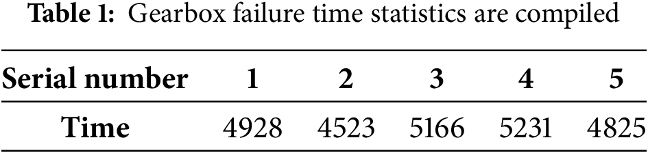
In this section, actual operation and maintenance data from a wind farm in Jiuquan is selected for simulation verification. Table 1 presents the lifespan data for five gearboxes, and Table 2 shows a portion of the monitoring data for Gearbox No. 4.

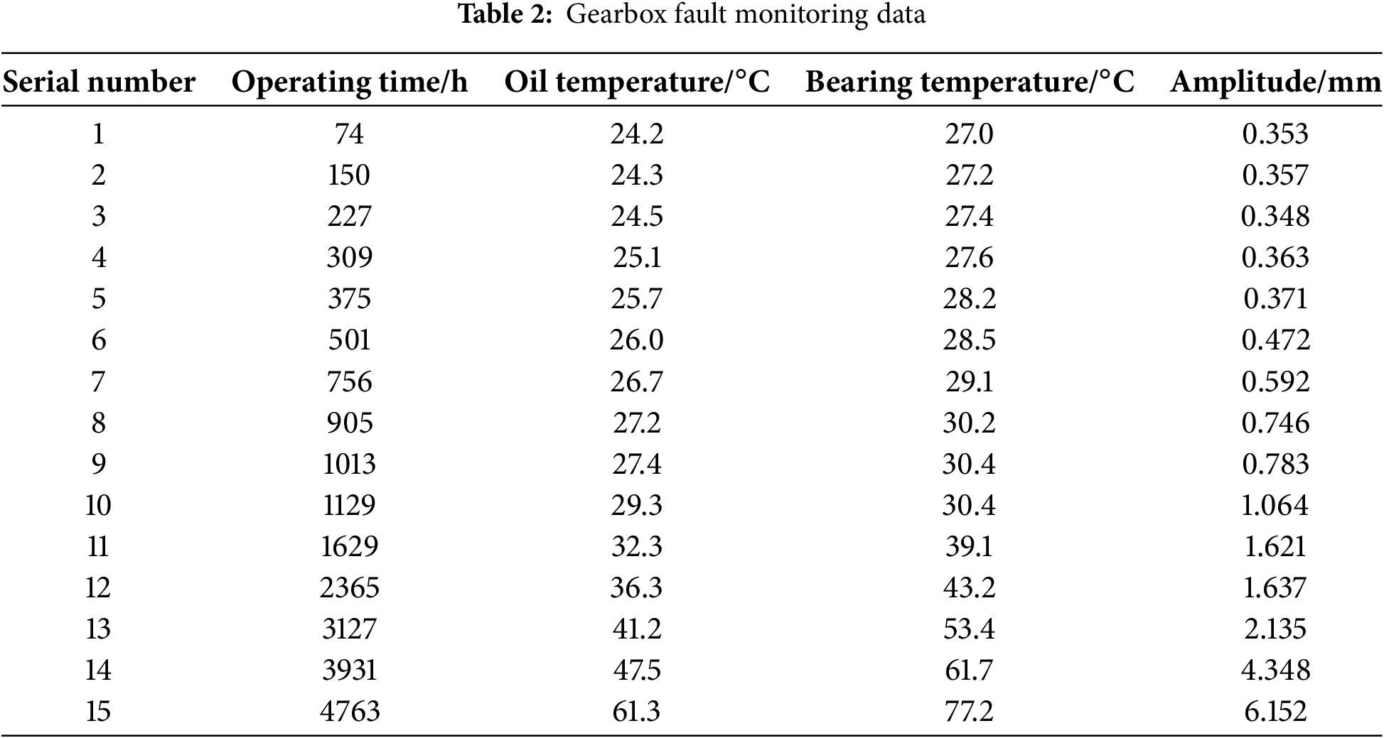
Due to the heterogeneity of units among the monitored indicators in the aforementioned dataset, the entropy weighting method [26] is employed to eliminate dimensional effects and assign weights to each indicator, thereby enabling the aggregation of multi-indicator data into a unified equipment condition index, denoted as x(t). Based on the monitoring data presented in Table 2, the following parameter values are obtained: β = 2.04; η = 10,258; ε = 0.43; k = 0.00127.

The condition-based degradation (CBM) model for the gearbox is formulated as shown in Eq. (23):

dx(t)=−2.0410258(t10258)1.04⋅11−0.43⋅x(t)dt+0.00127x(t)dB(t)(23)

By solving for the mean degradation rate, the time-based degradation (TBM) model is obtained as expressed in Eq. (24):

dx(t)=−[2.7316623(t16623)1.73⋅x∗(t)]dt(24)

The state degradation trajectories of the gearbox under Condition-Based degradation (CBM) and Time-Based degradation (TBM) models, as illustrated in Fig. 5, were obtained via MATLAB simulation. The actual condition of the gearbox was determined based on data processed by the Supervisory Control and Data Acquisition (SCADA) system.

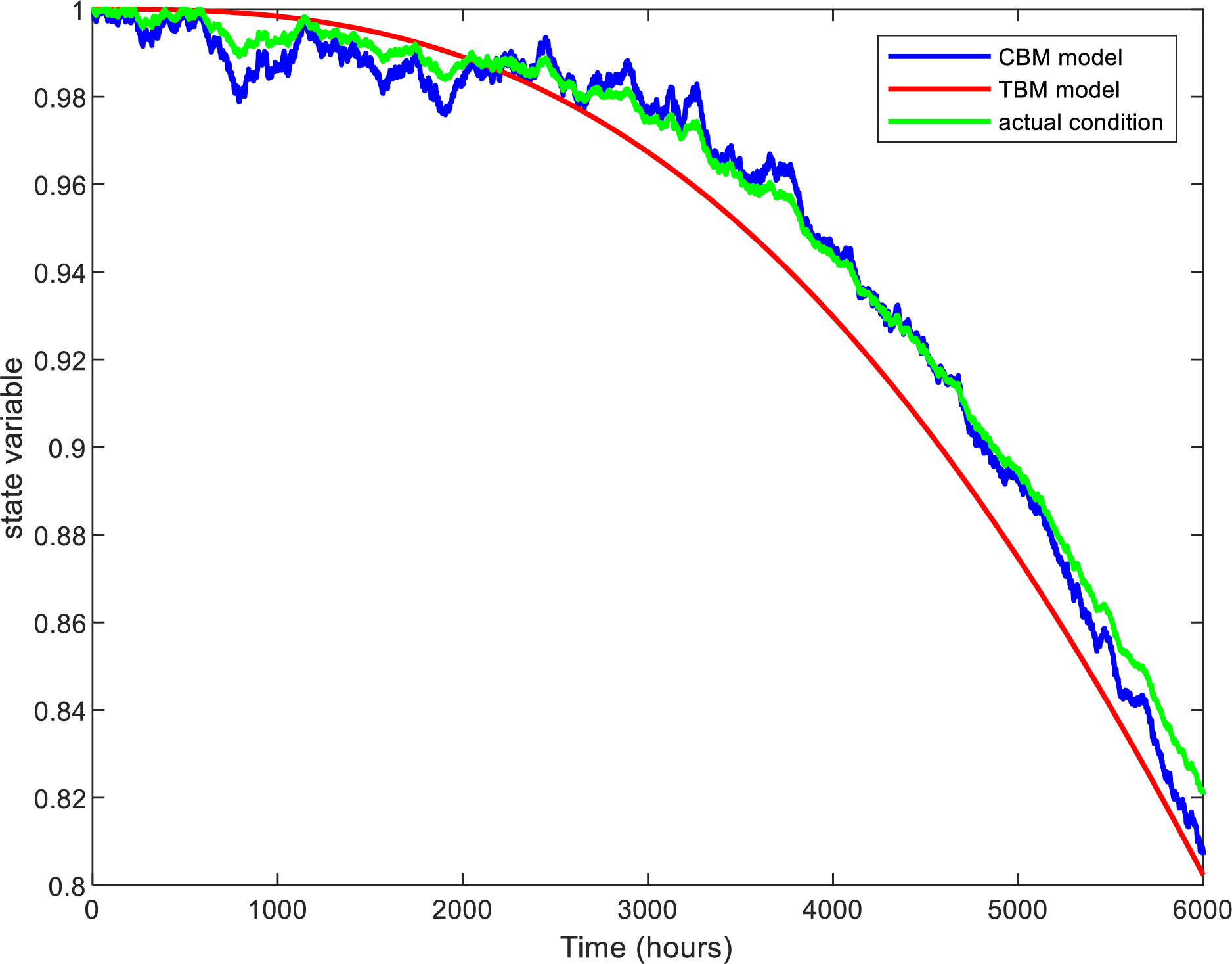
Figure 5: The principles of Time-Based Maintenance (TBM)

As demonstrated in Fig. 5, the CBM and TBM state degradation models constructed in this study based on stochastic differential equations (SDE) exhibit high consistency with the actual degradation trajectories of gearboxes, validating the effectiveness of the SDE framework in quantifying stochastic perturbations through Brownian motion terms and characterizing nonlinear deterioration via state influence rate functions. This approach significantly addresses the limitations of existing research in modeling equipment degradation stochasticity and acceleration trends. Compared to conventional ODE models, the stochastic differential terms in SDE endow state trajectories with independent increment properties, enabling instantaneous response to exogenous disturbances such as wind speed fluctuations and inspection impacts, thereby producing degradation curves that align with actual operational conditions. Furthermore, the SDE model rigorously ensures the existence and uniqueness of global solutions through Itô integral formulation, providing an analytical and iterative mathematical foundation for subsequent integration of reliability constraints, imperfect maintenance factors, and cost optimization. CBM, with its high sensitivity to stochastic disturbances, can promptly detect minute state variations, while TBM provides statistical benchmarks for scheduled maintenance through expected trajectories, synergistically optimizing the trade-off between state sensitivity and maintenance planning.

Fig. 6 illustrates multiple CBM sample trajectories alongside the state degradation curve of the TBM model.

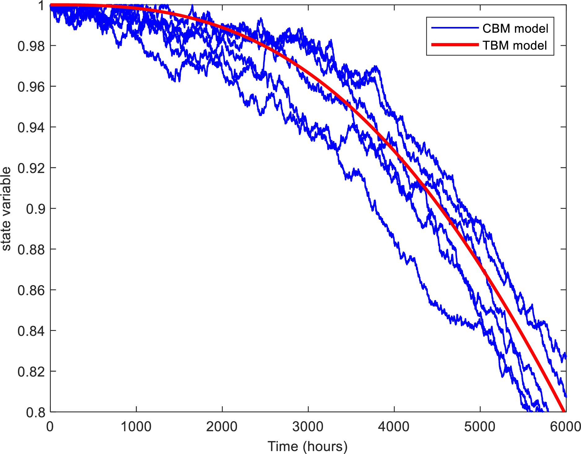
Figure 6: CBM multi-sample trajectory state evolution diagram

As shown in Fig. 6, the TBM degradation model curve represents the mean of several CBM sample trajectories, which is consistent with the theoretical analysis in Section 2.2.2, namely that the TBM constitutes the expectation of the CBM. This finding indicates that the TBM degradation model is not a simplistic fixed-interval maintenance strategy, but rather a statistical aggregation of multiple CBM sample trajectories, thereby capturing the overall trend of equipment state evolution. The CBM degradation model, by enabling real-time monitoring and maintenance decision-making, accurately characterizes the degradation process; however, the stochasticity of maintenance timing may result in insufficient preparation of maintenance resources. In contrast, the TBM degradation model, by modeling the expectation of the CBM, standardizes maintenance intervals and facilitates advance resource allocation, thereby addressing the unpredictability inherent in CBM-based scheduling. Consequently, the TBM degradation model integrates the state sensitivity of CBM with the schedulability of time-based approaches, effectively mitigating both under-maintenance and over-maintenance, and thus constitutes a scientifically robust and efficient maintenance methodology.

To further substantiate the advantages of the stochastic differential equation model proposed in this paper over the conventional ordinary differential equation models commonly employed in current research, the actual operational and maintenance data of the aforementioned gearbox were utilized. Specifically, λ(x(t), t) was represented using the widely adopted Weibull proportional hazards model, thereby constructing a standard ordinary differential equation-based state transition model for the gearbox, as shown in Eq. (25).

dx(t)=−λ(x(t),t)dt=−βη(tη)β−1exp⁡(ε⋅x(t))dt(25)

Using the parameter estimation method from Section 2.3.1, we obtained β = 2.72, η = 11,625, and ε = 0.25, which when substituted into Eq. (25) yields Eq. (26):

dx(t)=[−2.7211625(t11625)1.72e0.25x(t)]dt(26)

From Eq. (26), it is evident that the gearbox degradation process under this state model exhibits a smooth curve trajectory, which fails to capture the abrupt state transitions that occur when the gearbox encounters sudden operational conditions. In contrast, the stochastic differential equation model, leveraging the independent increment properties of Brownian motion, enables x(t) to approach any target value at time t. MATLAB simulation results demonstrate the residual distribution between the actual and predicted gearbox states, as illustrated in Fig. 7.

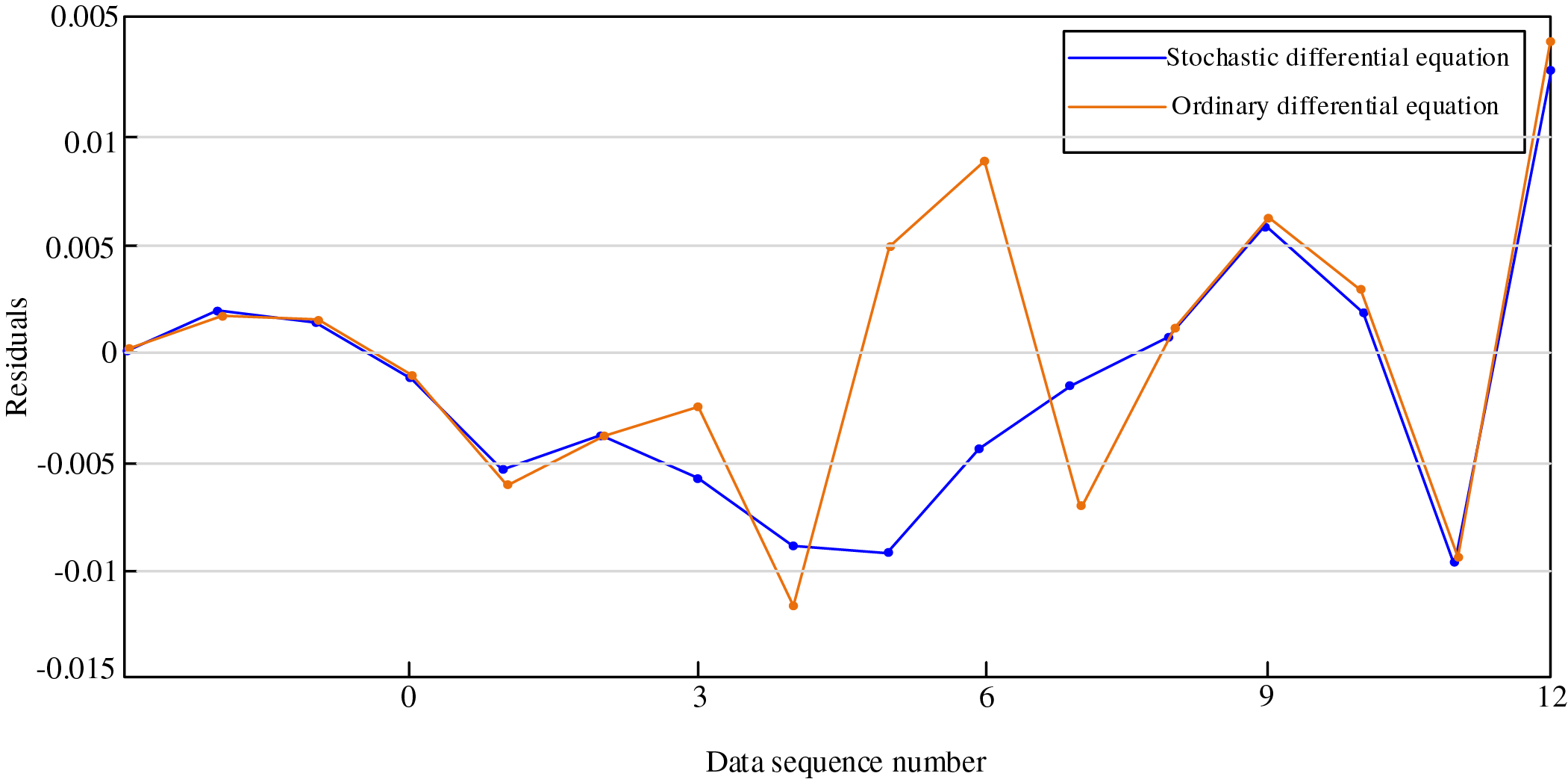
Figure 7: Residual distribution

Upon calculation, the mean residuals for the two maintenance models are 0.0043 and 0.0050, respectively. Comparative analysis reveals that the gearbox state transition model constructed using ordinary differential equations exhibits significant residual fluctuation amplitudes, indicating limited capability of existing models to track gearbox state evolution under transient operating conditions. Conversely, the stochastic differential equation model demonstrates substantially smaller residual variations. These findings validate that stochastic differential equations provide superior real-time equipment state characterization, exhibiting enhanced performance in both applicability and accuracy.

3  Development of a Time-Based Imperfect Maintenance (TBIM) Model

The aforementioned CBM and TBM degradation models constructed based on SDE employ replacement maintenance, whereby equipment is restored to an “as-good-as-new” condition post-maintenance. However, this “as-good-as-new” maintenance approach fails to adequately characterize the imperfect nature of maintenance effectiveness observed in engineering practice. Replacement maintenance of critical wind turbine components (such as gearboxes and bearings) encounters four fundamental contradictions: First, replacement maintenance involves prohibitively high costs and extended downtime, particularly problematic given that O&M costs constitute a substantial proportion of total costs in most wind farms, making excessive reliance on replacement maintenance significantly detrimental to economic viability. Second, wind turbine equipment failure degradation exhibits “progressive accumulation” characteristics—for instance, gear tooth surface wear and bearing fatigue crack propagation represent continuous and irreversible performance deterioration, with preventive maintenance typically unable to fully restore performance to as-new conditions. Third, complex systems (drivetrain, hydraulic systems, etc.) are constrained by current technological limitations, making complete elimination of component cumulative damage through single maintenance interventions challenging. Replacement maintenance models fail to account for such technological bottlenecks, whereas “imperfect maintenance” partial restoration modeling logic aligns maintenance effectiveness with actual technological feasibility. Fourth, wind farms frequently utilize weather windows (such as low wind speed periods) for multi-component coordinated maintenance, where time or resource constraints result in maintenance degradation, making “imperfect maintenance” implementation consistent with engineering reality.

To address these issues, the TBIM model proposed herein represents an innovation and improvement upon traditional replacement maintenance models. The TBIM model incorporates age reduction factors and failure rate growth factors to more accurately characterize actual equipment condition and performance variations post-maintenance. Furthermore, the TBIM optimization model in subsequent sections dynamically adjusts maintenance intervals to accommodate accelerated equipment degradation trends while comprehensively considering various maintenance costs to establish a comprehensive cost optimization framework, ensuring maintenance strategies are both cost-effective and reliable. This significantly improves upon traditional models that typically neglect the economic implications of maintenance decisions. These enhancements enable the TBIM model to outperform conventional replacement maintenance strategies in terms of economic efficiency, alignment with failure degradation characteristics, adaptability to maintenance technological constraints, and opportunistic maintenance resource integration, making it more suitable for actual wind turbine equipment O&M requirements.

3.1 Establishment of the TBIM Framework

Based on the aforementioned analysis, replacement maintenance restores equipment to an as-new condition; however, in practical engineering applications, replacement maintenance encounters challenges including prohibitive costs, extended downtime, technical constraints, and incompatibility with progressive degradation characteristics. Conversely, minimal repair exhibits the limitation of requiring multiple interventions while yielding marginal improvement in system performance. Consequently, this section incorporates two fundamental parameters into the TBM framework:

1.   The age reduction factor ai−1 (0 < ai−1 < 1) quantifies the mitigation effect of imperfect maintenance on equipment “virtual age”. Since maintenance of critical wind turbine components (such as gearboxes and bearings) cannot completely eliminate accumulated damage, post-maintenance equipment does not return to an as-new condition but rather achieves a “partially rejuvenated” state. For instance, ai−1 = 0.6 indicates that the equipment’s effective age is reduced to 60% of its pre-maintenance value, demonstrating the partial reversal of aging processes while acknowledging residual damage persistence.

2.   The failure rate escalation factor bi−1 (bi−1 > 1) characterizes the cumulative deterioration trend in equipment failure rates following multiple imperfect maintenance interventions. As maintenance frequency increases, internal component degradation accumulates progressively, diminishing the system’s resilience and accelerating failure rate progression. This factor amplifies the baseline failure rate in subsequent operational cycles (e.g., bi−1 = 1.2 indicates the failure rate in cycle i is 1.2 times that of cycle i − 1), accurately capturing the “maintenance-induced degradation” phenomenon inherent in wind turbine systems while circumventing the limitations of conventional models that treat post-maintenance failure rates as static parameters.

The ai−1 and bi−1 parameters are incorporated to establish an imperfect maintenance (TBIM) model, wherein post-maintenance equipment condition cannot be fully restored to its initial state, but rather remains in an intermediate condition between “as-good-as-new” and “as-bad-as-old” states. Furthermore, as operational time accumulates and imperfect maintenance events increase, the equipment failure rate exhibits a progressive upward trend. The fundamental relationship governing the change in failure rate before and after imperfect maintenance is expressed in Eq. (27):

hi(t)=bi−1hi−1(t+ai−1Ti−1)(27)

where i denotes the index of the imperfect maintenance cycle; hi(t) and hi−1(t) represent the baseline hazard rate functions for the ith and i − 1th cycles, respectively; Ti−1 indicates the time interval between two consecutive imperfect maintenance actions.

The quantification of service life degradation factor ai−1 and failure rate escalation factor bi−1 is derived from historical maintenance records of critical wind turbine components. By extracting empirical failure rate measurements before and after successive repairs of target components (e.g., gearboxes), correlational relationships between these factors and repair frequency as well as prior failure rate values are established. Least squares regression analysis is applied to the dataset to yield:

ai−1=(i−1)5(i−1)+9(28)

bi−1=13(i−1)+112(i−1)+1(29)

To more intuitively illustrate the variation in the failure rate function following the introduction of the age reduction factor ai−1 and the failure rate increase factor bi−1, the failure rate function for four imperfect maintenance cycles of a gearbox is presented in Fig. 8.

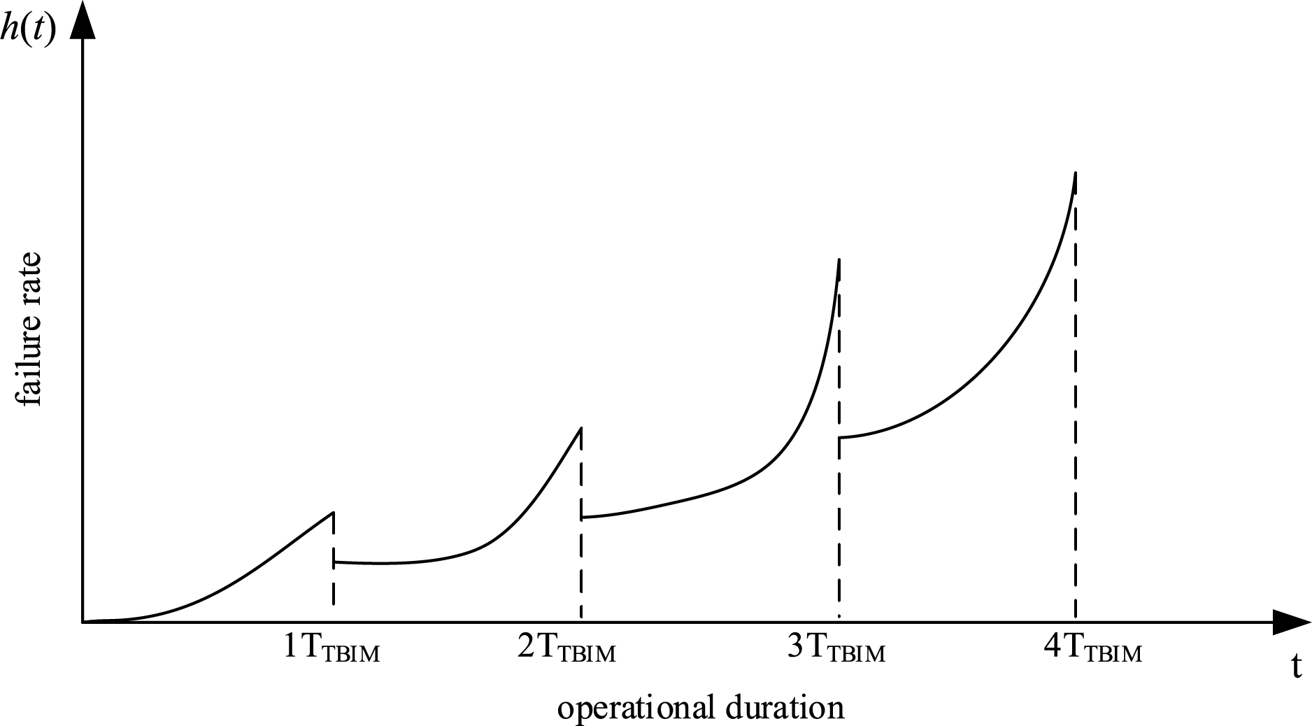
Figure 8: CBM multi-sample trajectory state evolution diagram

As illustrated in Fig. 8, under the synergistic mechanism of service age reduction factors and failure rate escalation factors, equipment exhibits pronounced “age regression” phenomena following each imperfect maintenance intervention. Specifically, the post-maintenance failure rate function does not reset to zero initial conditions as assumed under “good-as-new” restoration paradigms, but rather establishes non-zero baseline values predicated upon pre-maintenance degradation accumulation levels. This characteristic fundamentally differs from the idealized state where failure rate functions restart from zero under replacement maintenance, objectively revealing that imperfect maintenance corrections to equipment degradation processes constitute limited recovery based on practical engineering constraints (including maintenance resources, technical thresholds, and economic boundaries) rather than absolute restoration. This approach more accurately reflects the authentic state of maintenance behaviors in industrial scenarios—wherein maintenance operations cannot completely eliminate equipment’s historical degradation trajectories, but can only decelerate or modify degradation rates to a certain extent.

Further analysis reveals that failure rate function slopes exhibit monotonically increasing trends with accumulated imperfect maintenance implementations. This dynamic characteristic mathematically characterizes the intrinsic laws governing equipment performance evolution: following multiple maintenance interventions, equipment’s degradation resistance margins continuously diminish, with performance deterioration acceleration constantly increasing, ultimately manifesting significant accelerated degradation characteristics. This phenomenon not only validates the existence of diminishing marginal returns in imperfect maintenance’s long-term restoration effectiveness on equipment condition, but also provides critical evidence from a degradation dynamics perspective for understanding the correlation mechanisms between maintenance interventions and equipment reliability, establishing theoretical foundations for subsequent development of dynamic maintenance strategies that balance economic efficiency and reliability considerations.

As indicated by Eq. (27), the expression for hi(t) is altered exclusively following imperfect maintenance, while its continuity is preserved post-modification. Consequently, hi(t) may be regarded as a piecewise continuous function, as represented in Eq. (30).

{h1=b0h0(t+a0T0)h2=b1h1(t+a1T1)⋅⋅⋅hi=bi−1hi−1(t+ai−1Ti−1)(30)

Accordingly, the failure rate function is expressed as shown in Eq. (31):

λi(x(t),t)=hi(t)g(x(t))=∏i=1ibi⋅βη(t+aiTη)β−1⋅11−εx(t)(31)

Analogous to the TBM degradation model presented in Section 2.2.2, the TBIM model is also formulated as an ordinary differential equation. As established in the preceding analysis, each instance of imperfect maintenance results in a modification of the system’s failure rate function, and the equipment state cannot be restored to an “as-good-as-new” condition. Consequently, the TBIM state model can be represented as an n-stage ordinary differential equation, as expressed in Eq. (32):

{dx1(t)=−λ1(x(t),t)dtdx2(t)=−λ2(x(t),t)dt⋅⋅⋅dxn(t)=−λn(x(t),t)dt(32)

From the preceding analysis, it is evident that the time-based maintenance model represents the expected value of the condition-based maintenance model, wherein all pre-maintenance information is utilized to derive an average value of t, thereby establishing the maintenance interval for TBIM. Consequently, the temporal threshold for TBIM corresponds to the mean time under the CBM condition threshold, as demonstrated in Eq. (33):

TTBIM=E[E[τi|fτi]]=1n∑i=1nE[τi|fτi](33)

3.2 Empirical Validation and Analysis

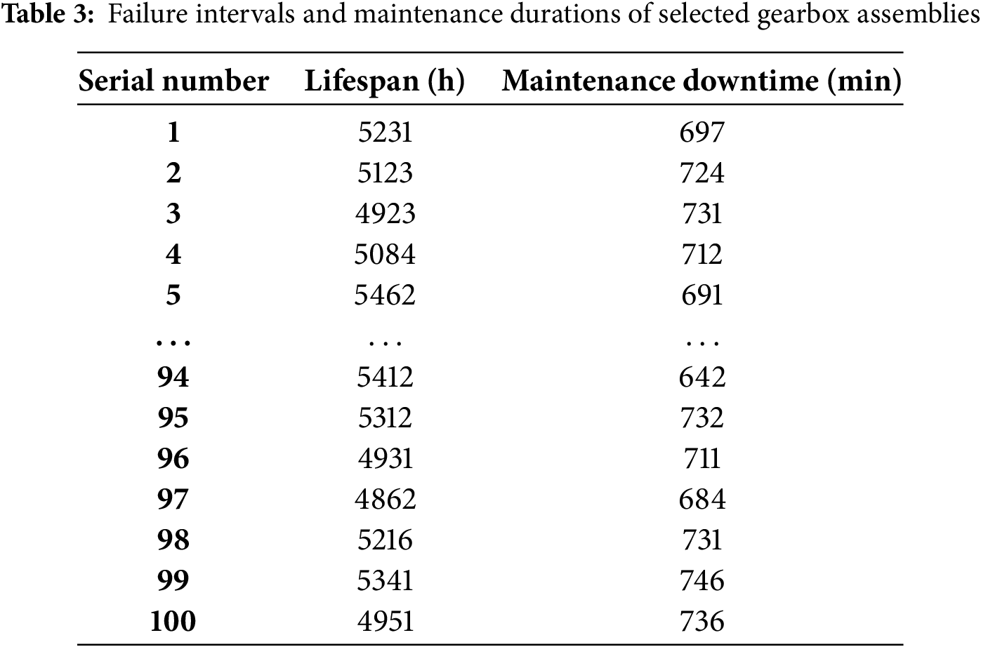
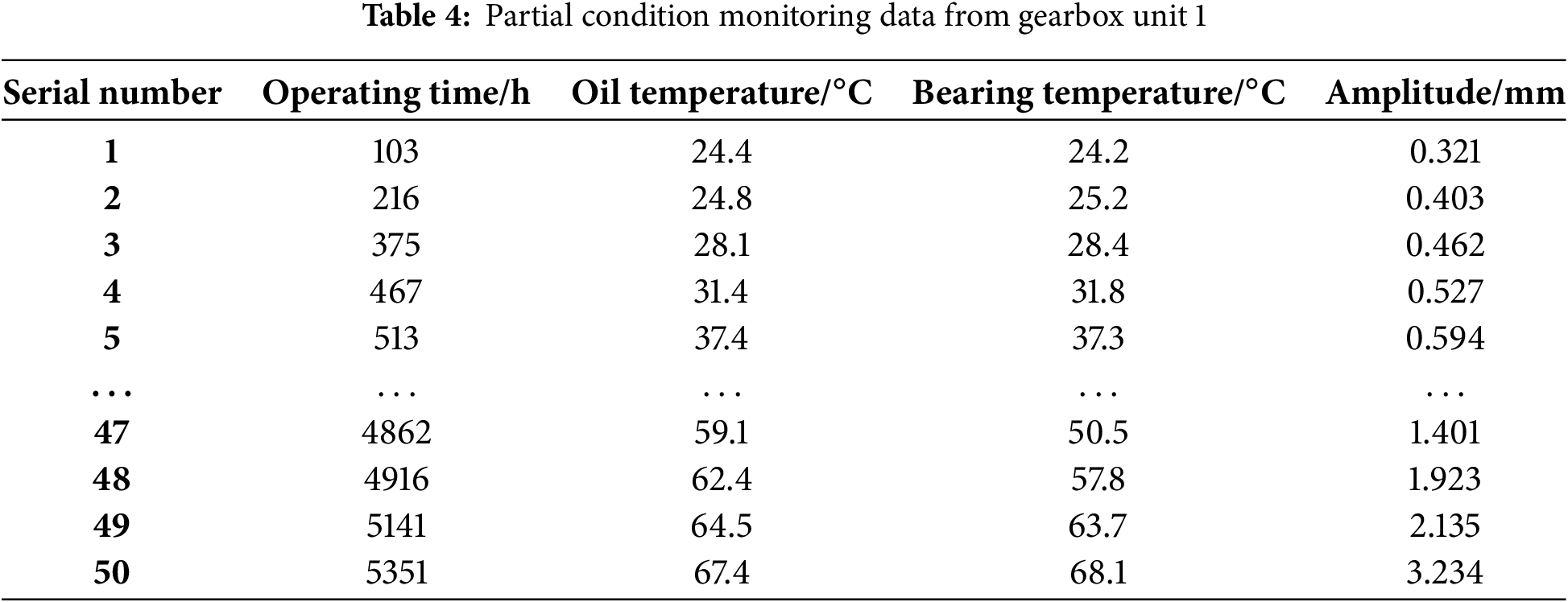
To validate the universal applicability of this study, this section employs monitoring data from identical gearbox components at a wind farm in Baiyin to verify whether the aforementioned model is applicable to real-world scenarios. Tables 3 and 4 present the failure times, mean downtime, and condition monitoring values for Gearbox No. 1 from identical gearbox units at the wind farm, respectively.

The parameter estimation and solution for this model yields h = 18,258, b = 2.03, ε = −0.41 from Section 2.3.1, while the time threshold for imperfect maintenance TTBIM = 3000 h is derived from Eq. (33) in Section 3.1. Consequently, the expression for the TBIM state model is obtained as:

dx(t)=(∏i=06bi⋅−2.0318258(t+3000ai10258)1.04)⋅11−0.41x(t)(34)

Fig. 9 illustrates the dynamic response characteristics of the gearbox operating under TBIM model conditions with Rp = 0.8, as determined through MATLAB simulation analysis.

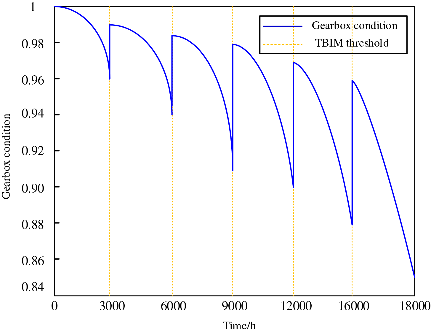
Figure 9: System states and maintenance strategies under the TBIM framework

As illustrated in Fig. 9, when the predetermined TBIM threshold is reached, imperfect maintenance is performed on the gearbox, whereby the equipment condition cannot be fully restored to an as-new state post-maintenance. For instance, upon reaching the TBIM threshold at the second occurrence (t = 6000 h), the equipment condition following imperfect maintenance satisfies x(6000) < x(t) < x(3000), indicating that the post-maintenance equipment performance lies between the pre-maintenance and pristine conditions. This demonstrates that the TBIM model accurately captures the condition evolution of equipment under imperfect maintenance scenarios, wherein each maintenance intervention yields partial restoration rather than complete renewal. Furthermore, as operational time progresses and maintenance frequency increases, equipment degradation exhibits an accelerating trend, which aligns with the observed condition evolution patterns of equipment following maintenance in practical engineering applications, thereby validating the efficacy of the TBIM model.

To further validate the advantages of the stochastic differential equation model incorporating imperfect maintenance, residual analysis was conducted using the dataset from this section. The stochastic differential equation model with imperfect maintenance was compared against both the Weibull proportional hazards ordinary differential equation model and the standard stochastic differential equation model. The residual plots depicting the discrepancies between predicted and observed states for these three distinct models are presented in Fig. 10.

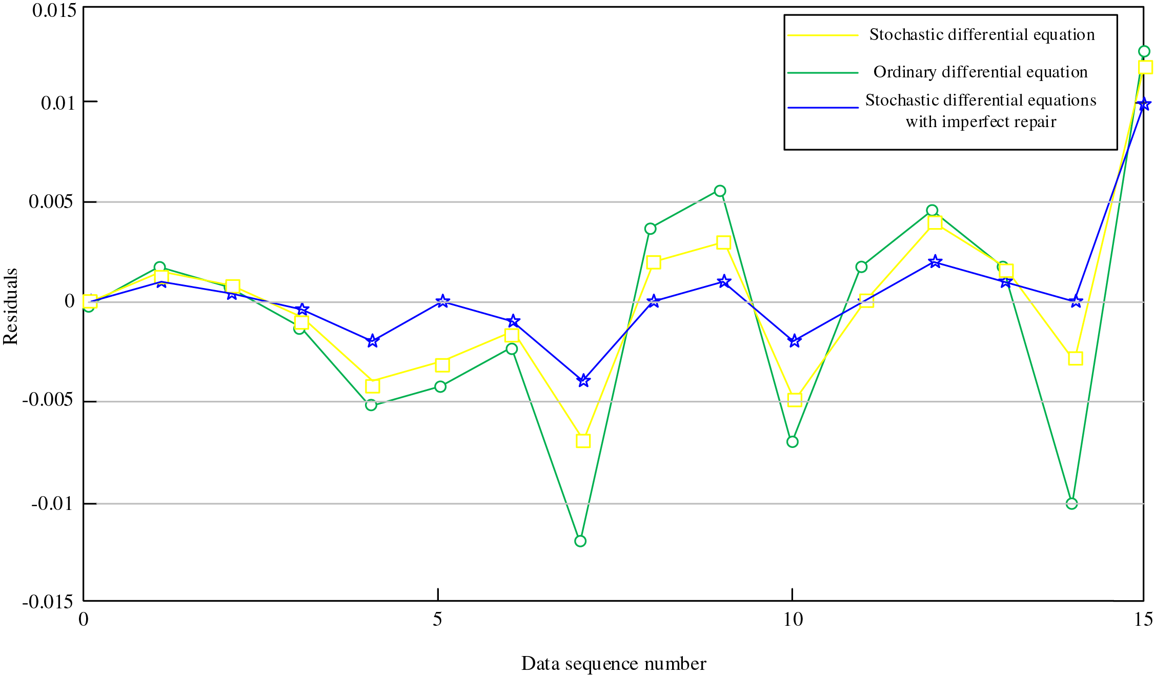
Figure 10: Residual distribution

Through computational analysis, the average residuals for the three models are 0.0050, 0.0047, and 0.0043, respectively. Analysis of Fig. 10 yields the following conclusions:

1.   When utilizing ordinary differential equations (ODE) to construct state equations, the state residuals exhibit significant discontinuities, making it challenging to accurately characterize equipment state transitions under non-standard operating conditions. In contrast, stochastic differential equations (SDE) demonstrate smaller residual values, enabling more precise reflection of actual equipment states for identical systems, thereby better aligning with practical equipment maintenance requirements. This finding corroborates the analysis presented in Section 2.3.2.

2.   Stochastic differential equations incorporating imperfect maintenance demonstrate superior performance in both residual characteristics and stability compared to conventional stochastic differential equations. This indicates that in actual wind turbine operations and maintenance, equipment states rarely achieve complete restoration to as-new condition through maintenance interventions, whereas imperfect maintenance represents a more feasible approach.

4  Optimization of the TBIM Mode

Although the TBIM model can more accurately characterize the actual condition and performance degradation of equipment post-maintenance through the incorporation of age reduction factors and failure rate growth parameters, further optimization remains necessary in practical implementation to enhance its economic efficiency and adaptability. Specifically, optimization of the TBIM model can better address the following challenges:

1.   Dynamic adaptability: The degradation process of wind turbine components exhibits stochastic and accelerating characteristics, making traditional fixed maintenance intervals inadequate for accommodating such variability. Therefore, reliability-constrained dynamic adjustment of maintenance intervals is required to better respond to accelerated equipment degradation trends.

2.   Cost-effectiveness: In operational practice, maintenance costs constitute a critical consideration. The TBIM model must minimize maintenance expenditures while ensuring high equipment reliability. This encompasses not only direct repair costs but also economic losses attributable to downtime.

Consequently, this chapter will comprehensively examine optimization methodologies for the TBIM model, including reliability-constrained dynamic maintenance interval adjustment and the development of an integrated cost optimization framework. Through these optimization strategies, the TBIM model can better accommodate the practical operational requirements of wind turbine systems while achieving optimal balance between economic efficiency and reliability performance.

4.1 Imperfect Maintenance Interval under Reliability Constraints

This section incorporates reliability thresholds Rp and Rr into the TBIM model, enabling dynamic maintenance interval adjustment based on equipment reliability. When equipment reliability degrades to Rp, imperfect maintenance is triggered; when reliability drops to Rr, replacement maintenance is executed. This dynamic adjustment mechanism effectively addresses accelerated equipment degradation trends while minimizing maintenance costs and ensuring high reliability. Through this approach, the TBIM model significantly enhances maintenance scheduling flexibility and adaptability, enabling superior response to actual operational and maintenance requirements of wind turbine equipment.

Based on the fundamental failure rate function of the Weibull distribution Eqs. (4) and (27), the baseline failure rate function of the optimized model under varying maintenance intervals Ti can be derived as follows in Eq. (35):

hi(t)=(∏k=1i−1bk)h(t+∑k=1i−1akTk)(35)

where hi(t) represents the baseline failure rate function for the ith cycle, and i denotes the number of imperfect maintenance cycles.

To ensure high-reliability operation of wind turbine generators. When the component reliability reaches Rp, imperfect maintenance is initiated, as expressed in Eq. (36):

exp⁡[−∫0T1h1(t)dt]=exp⁡[−∫0T2h2(t)dt]=⋯=exp⁡[−∫0Tihi(t)dt]=Rp(36)

Taking the logarithm of both sides of Eq. (36) yields Eq. (37):

∫0T1h1(t)dt=∫0T2h2(t)dt=⋯=∫0Tihi(t)dt=−ln⁡Rp(37)

According to Eq. (33), the probability of failure within each imperfect maintenance cycle is given by −lnRp. Therefore, based on Eqs. (31) and (33), the time interval for the ith imperfect maintenance cycle can be determined as follows in Eq. (38):

Ti=(∑k=1i−1akTk)β−ln⁡Rp×ηβ∏k=1i−1bkβ−∑k=1i−1akTk(38)

Within the cycle interval between the (i − 1)th and ith imperfect maintenance actions, the system reliability is:

Ri(t)=exp⁡[−∫0Tihi(t)dt](39)

After implementing the (n − 1)th imperfect maintenance on the component, its reliability is enhanced, and subsequently the reliability function Rn(t) begins to decline from unity. As system failure frequency increases, maintenance interventions become more frequent. When the reliability degrades from Rn(t) to the threshold value Rr, the system’s operational performance becomes inadequate, necessitating component replacement, specifically:

Rn(t)=exp⁡[−∫0Tnhn(t)dt]=Rr(40)

Based on Eqs. (35) and (40), the operational duration Tn of the equipment during the final cycle can be determined as shown in Eq. (41):

Tn=(∑k=1n−1akTk)β−ln⁡Rr×ηβ∏k=1n−1bkβ−∑k=1n−1akTk(41)

4.2 Optimization of Maintenance Costs

This section provides a comprehensive examination of constructing an integrated cost optimization framework that incorporates replacement maintenance, imperfect maintenance, and minimal repair costs, alongside downtime losses. Through dynamic adjustment of maintenance intervals and optimization of maintenance strategies, the TBIM model achieves substantial reduction in total maintenance costs while satisfying reliability requirements, thereby ensuring optimal equilibrium between economic efficiency and system reliability.

After incorporating reliability constraints into the TBIM model, replacement maintenance is implemented only when equipment reliability degrades to the replacement threshold Rr throughout the entire lifecycle. During other phases where reliability has not reached this threshold, a flexible combination of perfect maintenance and minimal maintenance is adopted based on equipment performance degradation levels and failure characteristics. Consequently, maintenance cost optimization must consider replacement maintenance costs (Cr), minimal maintenance costs (Cm), imperfect maintenance costs (Cf), and downtime losses per unit time (Cd).

1. Replacement Maintenance Cost

Let the replacement maintenance cost be denoted as Cr, and the duration of replacement maintenance as Tr.

2. Minimum Maintenance Cost

When equipment experiences minor malfunctions during operation that do not immediately affect normal functionality, emergency failures requiring rapid restoration of service, or components approaching end-of-life with low maintenance cost-effectiveness, minimal maintenance strategies should be implemented. Let the cost of a single minimal repair be denoted as Cm and the duration as Tm. If Ni represents the number of minimal repairs within each maintenance interval, then the cumulative minimal repair cost for all maintenance intervals prior to the nth maintenance cycle can be expressed by Eq. (42):

Cmn−1=Cm∑i=1n−1∫0Tihi(t)dt(42)

The minimum maintenance cost for the nth maintenance cycle is expressed in Eq. (43):

Cmn=Cm∫0Tnhn(t)dt(43)

Based on Eqs. (42) and (43), the minimum maintenance cost and corresponding time over the entire lifecycle are derived as:

TCm=Cm(∑i=1n−1∫0Tihi(t)dt+∫0Tnhn(t)dt)(44)

Tm=tm(∑i=1n−1∫0Tihi(t)dt+∫0Tnhn(t)dt)(45)

3. Imperfect Maintenance Cost

As operational time increases and the cumulative number of maintenance interventions rises, component wear and aging are exacerbated, resulting in increased maintenance complexity. Consequently, the cost of imperfect maintenance is abstracted into two components: a fixed cost Cc and a variable cost Cv Thus, the cost of the ith imperfect maintenance is expressed as shown in Eq. (46):

Cfi=Cc+iCv(46)

The preventive maintenance costs over the total maintenance cycle as:

TCf=∑i=1n−1Cfi=∑i=1n−1(Cc+iCv)(47)

Let τ denote the duration required for a single preventive maintenance action; thus, the total preventive maintenance time within one cycle is expressed as shown in Eq. (48):

Tf=(n−1)τ(48)

4. Downtime cost

From Eqs. (45) and (48) and the replacement maintenance duration, the total maintenance time over the entire life cycle can be determined as:

Tall=(n−1)τ+Tr+tm(∑i=1n−1∫0Tihi(t)dt+∫0Tnhn(t)dt)(49)

The total downtime loss is expressed as shown in Eq. (50):

TCd=Cd(Tr+Tf+Tm)=Cd[Tr+(n−1)τ]+Cd[tm(∑i=1n−1∫0Tihi(t)dt+∫0Tnhn(t)dt)](50)

The total maintenance cost of the equipment is expressed as shown in Eq. (51):

CT=Cr+TCf+TCd+TCm(51)

The complete life cycle of the equipment is represented as shown in Eq. (52):

T=∑i=1n−1Ti+Tn+Tall(52)

Under the premise of ensuring high system reliability, the optimal number of imperfect preventive maintenance actions, n, and the corresponding dynamic maintenance intervals, Ti, are determined by minimizing the average maintenance cost. Based on Eqs. (37), (51) and (52), the economic optimization objective function is formulated as shown in Eq. (53):

E[Ccost(n,Ti)]=(Cm+Cdtm)[(−ln⁡Rp)(n−1)−ln⁡(Rr)]+∑i=1n−1(Cc+iCv)+Cr+Cd[Tr+(n−1)τ]∑i=1n−1Ti+Tn+tm[(−ln⁡Rp)(n−1)−ln⁡(Rr)]+(n−1)τ+Tr(53)

In Eq. (53), the variables n and Ti are required to satisfy the following constraint conditions:

{Ri(t)⩾Rp,i=1,2,⋯,n−1Rn(t)⩾Rc∑i=1n−1Ti+Tn+tm[(−ln⁡Rp)(n−1)−ln⁡(Rr)]+(n−1)τ+Tf⩽TLtm(−ln⁡Rp)+τ≤Titm(−ln⁡Rp)+Tf≤Tn(54)

4.3 Analysis of Replacement Threshold Selection and Optimization Results in Case Studies

4.3.1 Selection of Replacement Threshold

This study establishes replacement thresholds based on reliability as the evaluation criterion, where the threshold magnitude influences both the operational duration of the final cycle and maintenance outcomes. Therefore, it is essential to rationally determine the replacement threshold Rr while ensuring equipment performance integrity, thereby maximizing residual service life utilization during the terminal operational cycle and optimizing maintenance expenditures. Based on expert judgment, if the reliability threshold for imperfect maintenance is set between 0.80 and 0.95, the replacement threshold should be less than 0.8. In this section, the gearbox discussed in Section 2.3.2 is used as a case study to determine the replacement threshold. The following assumptions are made regarding the maintenance durations for each strategy: minimal repair Tm = 2d days; replacement maintenance Tr = 15d days; imperfect maintenance τ = 8d days.

The maintenance costs associated with various gearbox maintenance strategies are presented in Table 5.

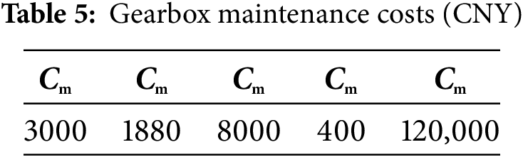
The variation in average maintenance cost corresponding to different replacement thresholds Rr ∈ [0.70, 0.75] under reliability thresholds Rp = 0.8 and Rp = 0.8, as determined by enumeration, is illustrated in Fig. 11.

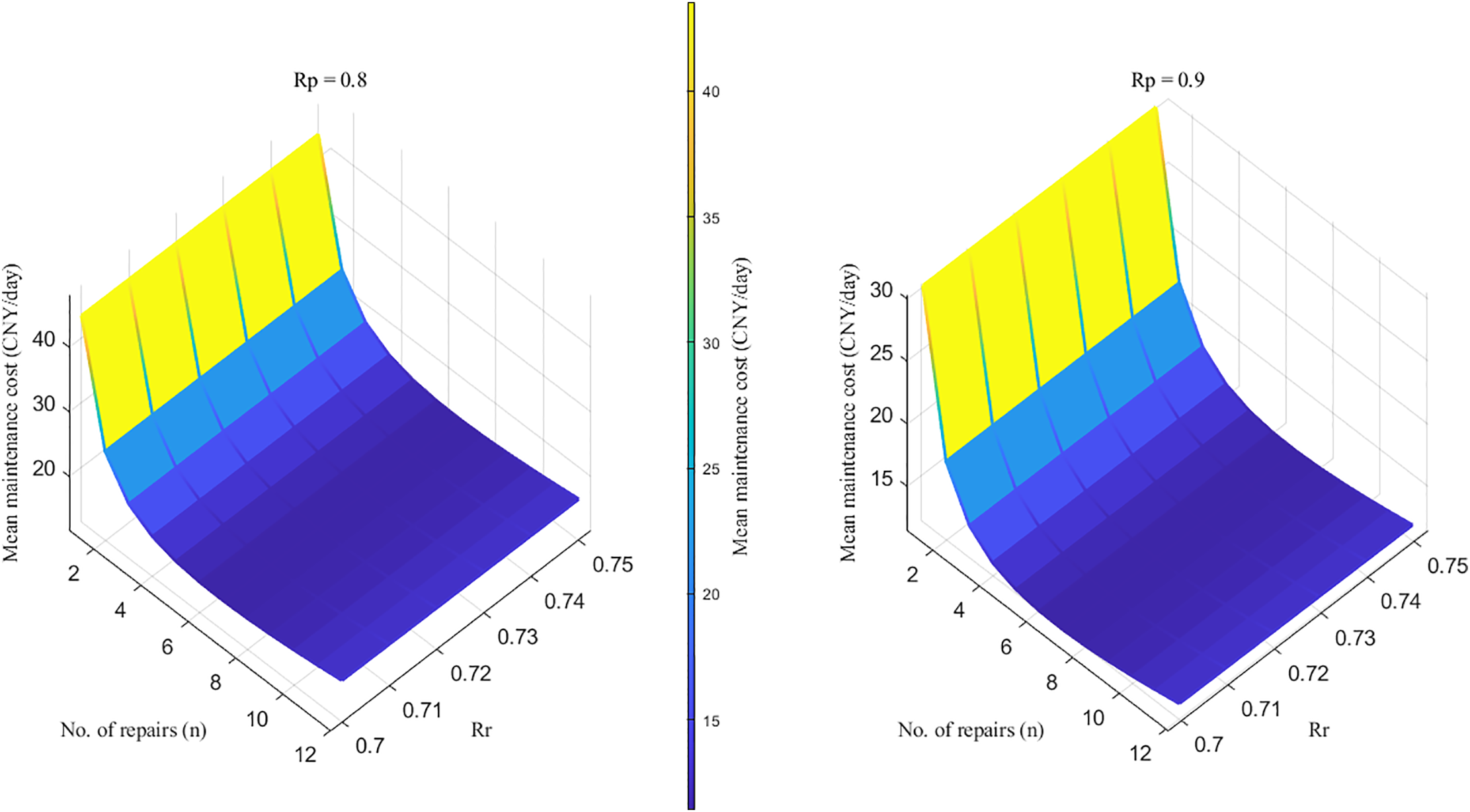
Figure 11: Mean maintenance cost variation diagram

As illustrated in Fig. 11, when the replacement threshold Rr remains constant, the average maintenance cost exhibits a U-shaped pattern, initially decreasing and subsequently increasing with the number of imperfect repairs. When the reliability threshold Rp and n are held constant, the average cost increases proportionally with higher Rr values. The aforementioned analysis demonstrates that at Rr = 0.70, both imperfect repair thresholds yield minimum average costs while maximizing equipment operational duration, thereby achieving optimal equilibrium between reliability and economic efficiency. Consequently, the replacement threshold is established at 0.7 in the proposed model.

4.3.2 Case Study Analysis

By setting the gearbox service life in Section 2.3.2 to 23,000 h and conducting simulation-based optimization within the finite time horizon, the maximum number of preventive maintenance actions, n, is determined to be 7. The expected maintenance cost for the partial maintenance policy, as derived from the model solution, is illustrated in Fig. 12.

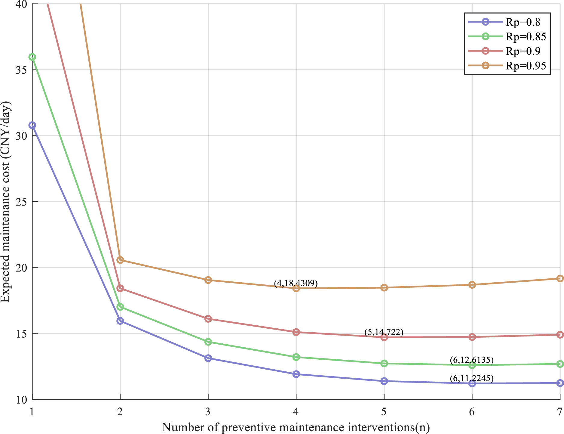
Figure 12: Maintenance costs under selective maintenance strategies

Analysis of Fig. 12 indicates that, under varying reliability threshold conditions, the relationship between expected maintenance cost and the number of imperfect maintenance actions exhibits a nonlinear trend: initially decreasing and subsequently increasing. Specifically, as the number of imperfect maintenance interventions increases, the expected maintenance cost declines during the initial phase; however, beyond a certain threshold, further increases in maintenance frequency result in elevated costs. This phenomenon suggests the existence of an optimal number of imperfect maintenance actions that minimizes the expected maintenance cost. For a fixed number of maintenance actions, the expected maintenance cost increases with higher reliability thresholds, attributable to the requirement for the system to maintain superior operational states, thereby necessitating more frequent or comprehensive maintenance and consequently incurring higher costs. For instance, when the reliability threshold Rp is set at 0.8, simulation results demonstrate that the expected maintenance cost reaches its minimum at six imperfect maintenance actions, indicating that exceeding this optimal value renders additional imperfect maintenance economically unjustifiable, and replacement maintenance should be considered.

This pattern demonstrates universality across different reliability thresholds, specifically indicating that regardless of the reliability threshold configuration, an optimal number of imperfect maintenance interventions exists that minimizes maintenance costs while ensuring equipment achieves the specified reliability level. In-depth investigation of the intrinsic relationship between expected maintenance costs and imperfect maintenance frequency can provide invaluable guidance for wind turbine maintenance decision-making. Through precise determination of imperfect maintenance intervals, maintenance costs can be substantially reduced while satisfying equipment reliability requirements, achieving synergistic integration and coordinated development of economic efficiency and equipment reliability.

5  Comparative Validation Analysis of Models

To further assess the practical effectiveness and cost-efficiency of the developed model, analyze the dynamic cycles and maintenance cost scenarios for this component under reliability parameters (Rp, n) of (0.80, 6) and (0.90, 5), respectively. this section continues to use the gearbox example from Section 2.3.2. Table 6 presents the changes in imperfect maintenance intervals and associated maintenance costs for the optimized TBIM model when (Rp, n) are set to (0.80, 6) and (0.90, 5), respectively.

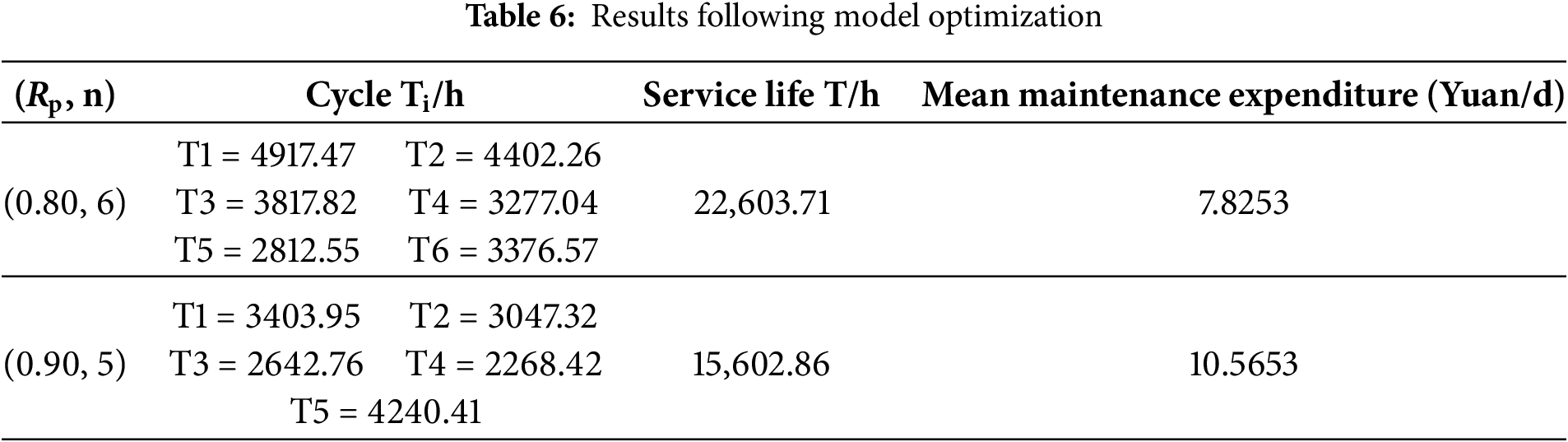
Analysis of Table 6 reveals that as the frequency of maintenance interventions increases, the imperfect maintenance intervals progressively diminish due to the combined effects of age-related degradation in baseline failure rates and temporal deterioration of equipment components. To sustain optimal reliability performance, higher reliability thresholds necessitate correspondingly shorter maintenance cycles and reduced operational lifespans, while concurrently elevating average maintenance expenditures.

Based on the optimized imperfect maintenance model (TBIM), simulation results demonstrate the gearbox condition and maintenance strategy evolution curves for decreasing intervals at Rp = 0.9, as illustrated in Fig. 13. This figure clearly reveals the dynamic evolution patterns of the optimized maintenance intervals. In fixed-interval models, maintenance schedules remain static and cannot adapt to actual equipment degradation states. Such rigid maintenance strategies may result in under-maintenance or over-maintenance, consequently increasing maintenance costs or compromising equipment reliability. In contrast, the optimized TBIM incorporates reliability constraints to dynamically adjust maintenance intervals based on actual degradation conditions, thereby more effectively addressing accelerated equipment deterioration trends.

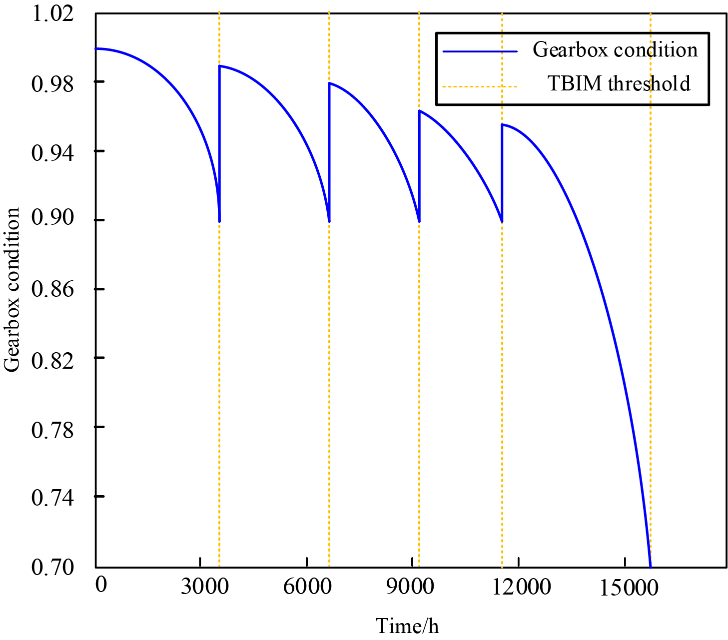
Figure 13: Status and maintenance strategies under the optimized TBIM model

Comparative analysis between the optimized model and the fixed-interval model without reliability constraints yields the following conclusions: When reliability threshold and preventive maintenance frequency combinations are set at Rp = 0.80, n = 6 and Rp = 0.90, n = 5, the fixed-interval model achieves equipment service lives of 18,000 h and 15,000 h, respectively, while the optimized TBIM extends service life to 22,603.71 and 15,602.86 h. These results demonstrate that the optimized model not only ensures equipment operation under high reliability conditions but also exhibits significant advantages in extending equipment service life. Furthermore, under Rp = 0.9 conditions, the optimized TBIM determines the optimal imperfect maintenance frequency as 5 cycles, with replacement maintenance implemented upon reaching this threshold. This pattern demonstrates strong concordance with the case study analysis in Section 4.3.2, further validating the effectiveness and economic viability of the optimized TBIM in practical applications.

When the replacement threshold Rc is not adjusted, equipment replacement is performed at the end of the final maintenance cycle when the reliability drops to the imperfect maintenance reliability threshold. The variations in imperfect maintenance intervals and associated maintenance costs for (Rp, n) values of (0.80, 6) and (0.90, 5) are presented in Table 7.

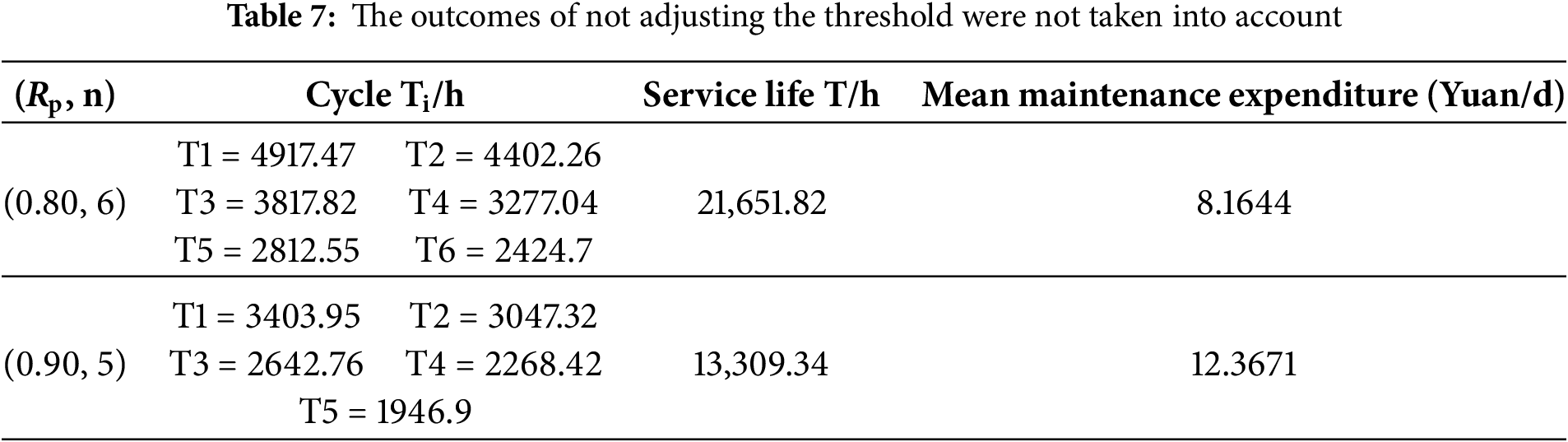
Analysis of data from Tables 6 and 7 demonstrates that implementing replacement threshold Rc achieves extended service life and reduced average maintenance costs across different reliability thresholds: at Rp = 0.80 and n = 6, service life increased by 951.89 h (4.4% improvement) while average maintenance costs decreased by 4.16%; at Rp = 0.90 and n = 5, service life increased by 2293.52 h (17.2% improvement) with average maintenance costs reduced by 14.6%. These findings indicate that incorporating replacement thresholds optimizes residual equipment life utilization while achieving cost-effective maintenance under reliability constraints.

6  Conclusion

This paper develops a wind turbine component degradation model and an imperfect maintenance optimization strategy (TBIM) based on stochastic differential equations (SDE). The principal findings are as follows:

1. Innovation in SDE-Based Modeling

A stochastic differential equation (SDE) modeling approach is proposed, incorporating random perturbation terms and state influence coefficients to address the inadequate characterization of equipment degradation fluctuations in conventional models. Gearbox data validation demonstrates that this model achieves superior fitting accuracy for actual degradation trajectories, while the time-based maintenance (TBM) model serves as the expected trajectory for condition-based maintenance (CBM), providing statistical theoretical foundation for periodic maintenance strategies.

2. Complementarity of CBM and TBM

The CBM model achieves precise maintenance triggering through real-time condition monitoring, yet stochastic maintenance intervals may result in resource allocation challenges; the TBM model addresses these limitations by averaging random perturbations and establishing fixed maintenance cycles based on CBM’s expected duration, thereby balancing condition-based responsiveness with maintenance schedulability to overcome the constraints of singular strategies.

3. Optimization Performance of the Imperfect Maintenance Model (TBIM)

The TBIM model incorporating age-reduction factors and failure rate escalation factors accurately characterizes the “as-good-as-old” performance degradation of equipment following maintenance interventions, establishing a non-periodic imperfect maintenance framework. A reliability-constrained preventive replacement maintenance methodology is proposed, providing computational formulations for determining replacement maintenance intervals in wind turbine components. Using wind turbine gearboxes as a case study, simulation analyses determined optimal preventive maintenance frequencies, maintenance intervals, and replacement cycles under varying reliability constraints. Comparative analysis with unconstrained reliability models and threshold-independent frameworks demonstrates that at an imperfect maintenance threshold of Rp = 0.80, gearbox operational lifespan increases by 4.4% while average maintenance costs decrease by 4.16%. Under high-reliability scenarios (Rp = 0.90), lifespan enhancement reaches 17.2% with cost reductions of 14.6%, achieving optimal equilibrium between wind turbine equipment reliability and economic efficiency.

4. Future Research Directions

This research can be further extended from single-component scenarios to multi-component degradation correlation modeling and coordinated maintenance strategy optimization for wind turbines, by developing multivariate degradation models to elucidate component coupling mechanisms and incorporating inventory theory to design joint “maintenance-inventory” optimization strategies, thereby enhancing overall operational efficiency of complex systems while achieving coordinated cost management.

Acknowledgement: Not applicable.

Funding Statement: This work was supported in part by the National Natural Science Foundation of China (No. 52467008) and Gansu Provincial Depatment of Education Youth Doctoral Suppo Project (2024QB-051).

Author Contributions: The authors confirm contribution to the paper as follows: study conception and design: Zhensheng Teng, Hongsheng Su; data collection: Zihan Zhou; analysis and interpretation of results: Zhensheng Teng, Hongsheng Su, Zihan Zhou; draft manuscript preparation: Zhensheng Teng. All authors reviewed the results and approved the final version of the manuscript.

Availability of Data and Materials: All data generated or analyzed during this study are included in this published article.

Ethics Approval: Not applicable.

Conflicts of Interest: The authors declare no conflicts of interest to report regarding the present study.

References

1. Jia M, Zhang Z, Zhang L, Zhao L, Lu X, Li L, et al. Optimization of electricity generation and assessment of provincial grid emission factors from 2020 to 2060 in China. Appl Energy. 2024;373(2):123838. doi:10.1016/j.apenergy.2024.123838. [Google Scholar] [CrossRef]

2. Xu J, Tao Y, Yang S, Zou J, Duan W, Chen Y, et al. High-resolution assessment of wind energy potential in the Hami region of Northwestern China. Environ Res Lett. 2024;19(12):124039. doi:10.1088/1748-9326/ad8bdd. [Google Scholar] [CrossRef]

3. Su X, Wang X, Xu W, Yuan L, Xiong C, Chen J. Offshore wind power: progress of the edge tool, which can promote sustainable energy development. Sustainability. 2024;16(17):7810. doi:10.3390/su16177810. [Google Scholar] [CrossRef]

4. Rozas H, Xie W, Gebraeel N. Condition-based maintenance for wind farms using a distributionally robust chance constrained program. IEEE Trans Power Syst. 2025;40(1):231–43. doi:10.1109/TPWRS.2024.3406335. [Google Scholar] [CrossRef]

5. Zhang X. Research on maintenance strategy optimization of metro train critical components based on competing weibull distribution [dissertation]. Nanning, China: Guangxi University; 2020. (In Chinese). doi: 10.27034/d.cnki.ggxiu.2020.002885. [Google Scholar] [CrossRef]

6. Zhou N, Luo L, Sheng G, Jiang X. Scheduling the imperfect maintenance and replacement of power substation equipment: a risk-based optimization model. IEEE Trans Power Deliv. 2025;40(4):2154–66. doi:10.1109/TPWRD.2025.3572076. [Google Scholar] [CrossRef]

7. Pedro K, Flores-Colen I, Ferreira C, Silva A. A comparative analysis of time- and condition-based approaches for imperfect maintenance of natural stone claddings. J Perform Constr Facil. 2024;38(5):04024025. doi:10.1061/jpcfev.cfeng-4764. [Google Scholar] [CrossRef]

8. Oh SY, Joung C, Lee S, Shim YB, Lee D, Cho GE, et al. Condition-based maintenance of wind turbine structures: a state-of-the-art review. Renew Sustain Energy Rev. 2024;204(4):114799. doi:10.1016/j.rser.2024.114799. [Google Scholar] [CrossRef]

9. Zhu X, Wang J, Coit DW. Joint optimization of spare part supply and opportunistic condition-based maintenance for onshore wind farms considering maintenance route. IEEE Trans Eng Manag. 2022;71(5):1086–102. doi:10.1109/TEM.2022.3146361. [Google Scholar] [CrossRef]

10. Byon E, Ding Y. Season-dependent condition-based maintenance for a wind turbine using a partially observed Markov decision process. IEEE Trans Power Syst. 2010;25(4):1823–34. doi:10.1109/TPWRS.2010.2043269. [Google Scholar] [CrossRef]

11. Wu X, Ryan SM. Optimal replacement in the proportional hazards model with semi-Markovian covariate process and continuous monitoring. IEEE Trans Reliab. 2011;60(3):580–9. doi:10.1109/TR.2011.2161049. [Google Scholar] [CrossRef]

12. Zhao X, Yang J, Qin Y. Optimal condition-based maintenance strategy via an availability-cost hybrid factor for a single-unit system during a two-stage failure process. IEEE Access. 2021;9:45968–77. doi:10.1109/access.2021.3067478. [Google Scholar] [CrossRef]

13. Liu Q, Ma L, Wang N, Chen A, Jiang Q. A condition-based maintenance model considering multiple maintenance effects on the dependent failure processes. Reliab Eng Syst Saf. 2022;220(3):108267. doi:10.1016/j.ress.2021.108267. [Google Scholar] [CrossRef]

14. Yuhan Li. Research on reliability-based maintenance decision for EMU gearboxes [master’s thesis]. Dalian, China: Dalian Jiaotong University; 2019. (In Chinese). doi: 10.26990/d.cnki.gsltc.2019.000508. [Google Scholar] [CrossRef]

15. Yi C, Wang H, Li J, Xie H. Rams-based comprehensive evaluation method for EMU components. Measurement. 2024;234(7):114821. doi:10.1016/j.measurement.2024.114821. [Google Scholar] [CrossRef]

16. Yu Q, Bangalore P, Fogelström S, Sagitov S. Optimal preventive maintenance scheduling for wind turbines under condition monitoring. Energies. 2024;17(2):280. doi:10.3390/en17020280. [Google Scholar] [CrossRef]

17. El-Naggar M, Sayed A, Elshahed M, EL-Shimy M. Optimal maintenance strategy of wind turbine subassemblies to improve the overall availability. Ain Shams Eng J. 2023;14(10):102177. doi:10.1016/j.asej.2023.102177. [Google Scholar] [CrossRef]

18. Fei SQ, Yuan TJ, Qi C, Zhai BY. Preventive maintenance strategy optimization of distributed energy supply equipment based on improved EWM-AHP. Acta Energiae Solaris Sin. 2023;44(4):341–8. (In Chinese). doi:10.19912/j.0254-0096.tynxb.2021-1510. [Google Scholar] [CrossRef]

19. Li JH, Jia S, Ren L, Li X. Research on wind turbines preventive maintenance strategies based on reliability and cost-effectiveness ratio. Ind Lubr Tribol. 2024;76(10):1168–76. doi:10.1108/ilt-05-2024-0153. [Google Scholar] [CrossRef]

20. Lopez JC, Kolios A, Wang L, Chiachio M, Dimitrov N. Reliability-based leading edge erosion maintenance strategy selection framework. Appl Energy. 2024;358(11):122612. doi:10.1016/j.apenergy.2023.122612. [Google Scholar] [CrossRef]

21. Lin J, Lan B, Chen W, Pei T, Zhu J. Opportunistic maintenance strategy for wind turbine systems based on fault correlation and multi-level maintenance theory. Electr Eng. 2025;107(4):5149–62. doi:10.1007/s00202-024-02819-5. [Google Scholar] [CrossRef]

22. Yi CS, Wang H. Preventive maintenance strategy for electric multiple unit components considering RAMS. J Harbin Eng Univ. 2025;46(2):309–19. (In Chinese). [Google Scholar]

23. Zhang G, Wang Y, Guo L, Qin Y, Tang B, Shao H. Slice-oriented signal probability distribution measure for wind turbine generator bearing condition monitoring under variable speed conditions. IEEE Trans Ind Inform. 2024;20(4):5297–307. doi:10.1109/TII.2023.3333844. [Google Scholar] [CrossRef]

24. Szubartowski M, Migawa K, Borowski S, Neubauer A, Hujo Ľ, Kopiláková B. Application of the semi-Markov processes to model the enercon E82-2 preventive wind turbine maintenance system. Energies. 2024;17(1):199. doi:10.3390/en17010199. [Google Scholar] [CrossRef]

25. Huangfu L. Research on condition evolution model and preventive maintenance decision method for repairable EMU components based on stochastic differential equations. Lanzhou, China: Lanzhou Jiaotong University; 2023. (In Chinese). doi:10.27205/d.cnki.gltec.2023.000020. [Google Scholar] [CrossRef]

26. Su H, Dong L, Yu X, Liu K. Research on carbon emission for preventive maintenance of wind turbine gearbox based on stochastic differential equation. Energy Eng. 2024;121(4):973–86. doi:10.32604/ee.2023.043497. [Google Scholar] [CrossRef]