
 Submit a Paper
 Propose a Special lssue
 Open Access
ARTICLE

Multi-Time Scale Optimization Scheduling of Data Center Considering Workload Shift and Refrigeration Regulation
China Energy Engineering Group Guangdong Electric Power Design Institute Co., Ltd., Guangzhou, 510700, China
* Corresponding Author: Luyao Liu. Email:
(This article belongs to the Special Issue: Innovative Renewable Energy Systems for Carbon Neutrality: From Buildings to Large-Scale Integration)
Energy Engineering 2026, 123(2), 20 https://doi.org/10.32604/ee.2025.072631
Received 31 August 2025; Accepted 06 November 2025; Issue published 27 January 2026
 View Full Text
 Download PDF
Abstract
Data center industries have been facing huge energy challenges due to escalating power consumption and associated carbon emissions. In the context of carbon neutrality, the integration of data centers with renewable energy has become a prevailing trend. To advance the renewable energy integration in data centers, it is imperative to thoroughly explore the data centers’ operational flexibility. Computing workloads and refrigeration systems are recognized as two promising flexible resources for power regulation within data center micro-grids. This paper identifies and categorizes delay-tolerant computing workloads into three types (long-running non-interruptible, long-running interruptible, and short-running) and develops mathematical time-shifting models for each. Additionally, this paper examines the thermal dynamics of the computer room and derives a time-varying temperature model coupled to refrigeration power. Building on these models, this paper proposes a two-stage, multi-time scale optimization scheduling framework that jointly coordinates computing workloads time-shift in day-ahead scheduling and refrigeration power control in intra-day dispatch to mitigate renewable variability. A case study demonstrates that the framework effectively enhances the renewable-energy utilization, improves the operational economy of the data center microgrid, and mitigates the impact of renewable power uncertainty. The results highlight the potential of coordinated computing workloads and thermal system flexibility to support greener, more cost-effective data center operation.Keywords
Artificial Intelligence (AI) has experienced explosive growth in recent years and plays a pivotal role in improving productivity and driving economic development. Under this background, data has increasingly emerged as a primary factor of production, and society is rapidly transitioning into the digital economy era that stimulates unprecedented demand for computational capacity. Data centers, functioning as the backbone for data processing and storage, are thus emerging as vital socio-economic infrastructure during this transition [1].
The data center industries are facing huge energy challenges due to their high power consumption and carbon emissions. Worldwide, data centers consume approximately 460 TWh of electricity annually, comprising nearly 2% of the global electricity use [2]. With world’s over 8000 data centers, the United States, Europe, and China host a significant portion of these facilities, which are 33%, 16% and 10%, respectively. In 2022, US data centers consumed 200 TWh of electricity, accounting for about 4% of the national electricity consumption. China’s data center electricity consumption reached 216.6 TWh, roughly 2.6% of the societal electricity consumption in 2021. The CO2 emissions from data centers reached 135 million tons, approximately 1.14% of the national emissions [3]. Emerging AI models with billions of parameters demand enormous energy during their training, and as AI technology evolves, data centers’ power consumption and carbon emissions will continue to grow [4]. In the pursuit of carbon neutrality, the integration of data centers with renewable energy sources has emerged as an inevitable trend [5]. China’s ‘Channeling computing resources from the east to the west’ policy was introduced against this backdrop, aiming to optimize the data-center layout and promote green energy utilization by leveraging the abundant wind and solar resources of the western regions [6].
To effectively integrate the intermittent renewable energy, it is essential to extensively analyze the operation flexibility of data centers [7]. Fig. 1 illustrates the structural overview of a green data center micro-grid. The information technology (IT) equipment mainly includes the servers that provide computing resource for workloads. The refrigeration system provides cooling resources to extract the heat generated from the IT equipment. The power infrastructure connects the wind, photovoltaic (PV) power system and main-grid in supply side and IT equipment, refrigeration system in power demand side.
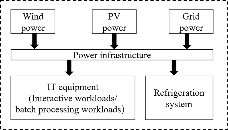
Figure 1: Structure of green data center
Data centers manage an exponentially increasing volume of computational workloads driven by continuous enhancements in processing capabilities. As computing workloads migrate across the network in temporal and spatial domains, the associated power consumption of the data center correspondingly varies. Thus, computing workloads exhibit significant spatiotemporal adjustable characteristics [8]. Additionally, computer room temperature can fluctuate within predefined limits, and the temperature change exhibits a temporal delay relative to the cooling power change. By dynamically modulating the refrigeration power within acceptable temperature bounds, fluctuations in renewable energy generation can be effectively managed [9]. Consequently, the refrigeration system functions as an auxiliary flexible resource for data center micro-grid operations.
This study concentrates on formulating power regulation models for delay-tolerant computing workloads and refrigeration system within data centers, and incorporating these flexible regulation models into power scheduling framework of data centers to increase the operational economy and maximize the utilization of renewable energy. Section 2 reviews pertinent literature to delineate the existing state of research and to identify critical knowledge gaps.
In recent studies, leveraging the spatiotemporal flexibility of computing workloads in data centers to promote renewable energy utilization has emerged as a new research focus. Chen et al. [10] analyzed the topology of computing power networks from an energy perspective, and used price leverage to guide the spatial shift of workloads from interconnected data centers to promote the renewable energy utilization and improve the grid resilience. Yang et al. [11] proposed a spatial migration mechanism of computing workloads based on the spatiotemporal distribution complementarity of renewable energy in multiple regions around the world, and conducted simulations using Google’s interconnected multiple data centers to minimize carbon emissions. However, the aforementioned research focuses mainly on the spatial redistribution of computing workloads across multiple data centers, with limited attention to the temporal shift of workloads within individual data centers.
The flexibility of computing workloads within an individual data center primarily manifests in their temporal transferability. According to the length of response delay, workloads can be categorized into delay-sensitive and delay-tolerant types [12]. Delay-sensitive workloads primarily refer to ‘online tasks’, or ’interactive workloads’ that provide real-time feedback to users. Delay-tolerant workloads, by contrast, refer to ‘offline tasks’ or ‘batch processing workloads’ that execute a series of jobs based on a computer program without human intervention; Their maximum response time can range from several minutes to days [13]. By dynamically adjusting the delay-tolerant workloads’ start time and the amount of computation load for each time interval within the response deadline, the power consumption of workloads can be controlled. This study concentrates on the temporal flexibility of workloads within an individual data center.
Studies regarding the temporal flexibility modeling of delay-tolerant workloads within an individual data center have been conducted. Liu et al. [14] proposed a power consumption model for the delay-tolerant workloads and integrated it with a renewable power supply model. The optimal plan of generator units’ outputs and workloads scheduling was obtained with the objective of minimizing operation cost of data centers. Cupelli et al. [15] simulated the power consumption of delay-tolerant workloads considering their arrival, queuing, and execution process. By coordinating workloads scheduling with cooling systems and energy-storage devices, they demonstrated reductions in overall data-center energy costs. Kwon [16] analyzed the time-shift characteristics of a simple delay-tolerant workload and developed a flexible mechanism model to shift workloads power consumption towards periods of high renewable generation. The studies above highlight the potential of delay-tolerant workloads to provide flexible regulation in individual data centers.
However, existing studies have primarily focused on modeling single, simple time-shiftable workload and haven’t comprehensively accounted for multiple time-shiftable workload types with distinct operational characteristics and shifting behaviors. Comprehensive modeling of multiple delay-tolerant workloads, and systematic integration of these models into data center power dispatch frameworks, remain insufficiently explored.
Furthermore, the refrigeration system serves as an additional flexible resource in data center operations. Data centers commonly employ refrigeration systems to maintain suitable thermal conditions. With advancements in technology, the temperature requirements for server clusters have become less stringent. The ASHRAE introduced the ‘Data Center Environmental Thermal Guidelines’ in 2014, extending the design ranges for maximum allowable computer room temperatures to 32°C, 35°C, 40°C, and 45°C across A1–A4 classifications. Considering the temperature fluctuation range and thermal inertia, existing research investigated the feasibility of utilizing refrigeration modulation to optimize data center operation. Tang et al. [17] established the first-order equivalent thermal parameter model to analyze the thermal load dynamics of the air condition system in base stations. By incorporating temperature variation boundaries, they employed day-ahead demand response strategies utilizing start-stop control to manage cooling and heating loads. Zhu et al. [18] formulated a temperature response model considering thermal inertia within data center environments and proposed dynamic temperature regulation strategies to optimize real-time renewable energy utilization. These investigations demonstrate the potential of using temperature and refrigeration modulation to enhance power scheduling efficiency in data centers. However, they don’t address the coordination of computing workloads time-shift and refrigeration modulation in data center operational management.
In light of the deficiencies, this research aims to provide a power scheduling framework for data center by incorporating the computing workloads shift and refrigeration regulation. To this aim, this work first analyzes the time-shift characteristics of three kinds of typical delay-tolerant computing workloads and establishes the corresponding time-shift models. Then, this work quantitatively examines the heat transfer process of data center and builds the time-variant model of computer room temperature. Last, this work proposes a two-stage multi-time scale optimization scheduling framework for the green data center, where the time-shift models of workloads are incorporated into the day-ahead optimization scheduling, and the refrigeration power is set as the control variable in the intraday scheduling. The proposed multi-time scale energy management method is applied to a data center to verify its effectiveness.
3.1 Time-Shift Models of the Delay-Tolerant Workloads
This section introduces three kinds of delay-tolerant workloads, i.e., Long-running non-interruptible, long-running interruptible, and short-running workloads, and models the time-shifting processes of the workloads.
3.1.1 Workloads Classification and Time-Shift Characteristics Analysis
Time-shiftable workloads are categorized into long-running and short-running workloads, distinguished by their processing time length. Long-running workloads include continuous non-interruptible and interruptible workloads based on their interruptibility.
Analysis of large internet data centers shows that processor resource consumption of computing workloads follows a heavy-tailed distribution, indicating that a small portion of long-running workloads consume a significant amount of processor resources [19]. These energy-intensive long-running workloads present opportunities for power regulation. Additionally, analysis reveals that most workloads in Google’s cluster last only a few minutes [19], while over 90% of batch jobs in Alibaba’s data cluster run for less than 15 min [20]. Short-running computing tasks, when combined, can effectively help mitigate fluctuations in renewable energy.
• Long-running non-interruptible workload
Some workloads, e.g., continuous integration and continuous deployment jobs (CI/CD), test suites, compilation jobs, database migration, and backups, can’t be paused or interrupted once execution begins and must run continuously until completion. Workload with this working characteristic are identified as ‘long-running non-interruptible workload’.
The temporal mitigation pattern for this kind of workload is to shift the overall workload within a certain time range while keeping the original shape of the computing power load curve unchanged.
• Long-running interruptible workload
Certain workloads, e.g., machine learning training, block-chain mining, protein folding, or long-running scientific simulations, can be paused or interrupted during execution and resumed at an appropriate time. Workload with this working characteristic is regarded as ‘long-running interruptible workload’.
According to its time-shift characteristics, long-running interruptible workload can be viewed as a holistic task comprised of multiple sequential subtasks. The shift strategy is to adjust each subtask forward or backward to a certain time point within a specified time frame, while ensuing the sequential order dependency among the subtasks.
• Short-running workloads
Some workloads, including function as a service, scheduled data backups, log cleaning, report generation, email or notification sending, etc., typically require brief execution time and don’t demand immediate response. These workloads can tolerate delays ranging from minutes to several hours, classifying them as short-running workloads.
Short-running workloads exhibit two defining characteristics: short execution duration and high task volume. When numerous short-running workloads aggregate, they form a short-running workload cluster, which presents significant potential for power regulation. The time-shifting mechanism for managing these workloads involves rescheduling all or part of the short-running tasks from their original time slots to alternative periods in future time window for execution.
3.1.2 Modelling of Long-Running Non-Interruptible Workload
Set the day-ahead scheduling period to 24 h, and define the scheduling time step as
where
where
The mitigation pattern for the long-running non-interruptible workload is to shift the entire workload along the time axis. Once the start time of the workload is determined, the computing power demand for each subsequent time point can be uniquely ascertained. Therefore, the pivotal parameter for the time-shift modelling of long-running non-interruptible workload is the time-shift vector of start node.
Use
where the element
For
The time at which the start node is positioned is denoted as
The long-running non-interruptible workload has the earliest start time point
The relation between the computing power demand time series of workload after shifting
where the dimension of
3.1.3 Modelling of Long-Running Interruptible Workload
Introduce
where
According to the time-shift characteristics of long-running interruptible workload, this study considers the long-running interruptible workload as a holistic task composed of multiple subtasks in sequence. The duration of each subtask is consistent with the scheduling time step
Hence, the original computing demand time series of the long time interruptible workload
In this vector, there exists a period of time with computing power demand value, and the elements before and after this period are zero.
The mitigation pattern for the long-running interruptible workload is scheduling individual subtasks to new time points within a specified time frame while preserving their sequential dependencies. Once the execution time of each subtask is determined, the computing power demand for the workload can be uniquely ascertained. Thus, the key parameter for time-shift modelling of long-running interruptible workload is the time-shift matrix of its subtasks.
Use
For each column in matrix
The matrix of time points where subtasks locate after shifting is denoted as
The computing power demand time series of each subtask after shifting is denoted as
3.1.4 Modelling of Short-Running Workloads
Introduce
where
The time shifting pattern for short-running workloads is shifting all or part of the tasks from the original time periods to new time periods. The key parameter for the time shift modelling of short-running workloads is the time shift matrix of the inflow and outflow amount of computing power demand at each time point.
Use
In this formula,
To illustrate the specific form of
M is a constant, equal to the peak computing power demand
Another constraint for
To prevent invalid shifting, a penalty cost coefficient matrix
The penalty cost function
where
3.1.5 Relation of Computing Power and Electricity Power
Computing power refers to a device’s capability to perform data processing and generate specific outputs. The computing power is implemented through various computing chips such as CPU, GPU, FPGA, ASIC, which are carried by computers, servers, and other systems. The standard measurement for computing power is the number of FLoating-point Operations executed Per Second (FLOPS).
The computing power of a chip is determined by three key factors: the number of computing cores of the chip
The computing power capacity of the data center
where
Based on the assumption that: (1) all servers in the data center are homogeneous; (2) all servers in the computer room are turned on. The power consumption of servers can be modelled as Eq. (30) [21,22]:
where
The formula for calculating CPU utilization is
where
This model provides a quantitative approach to estimate the electricity power consumption of workloads based on their computing power demand.
3.2 Time-Variant Model of Computer Room Temperature
Data center computer room temperature is influenced by multiple factors including server cluster heat generation, environmental maintenance structure, heat load, cooling power, and outdoor temperature. To simplify the problem-solving process when constructing a thermal model for the data center, the heat transfer through the walls is treated as a one-dimensional problem, and the physical properties of the walls is assumed to be remain constant over time. In addition, the indoor temperature is represented as a single node. The simplified heat transfer process for the data center room is depicted in Fig. 2.
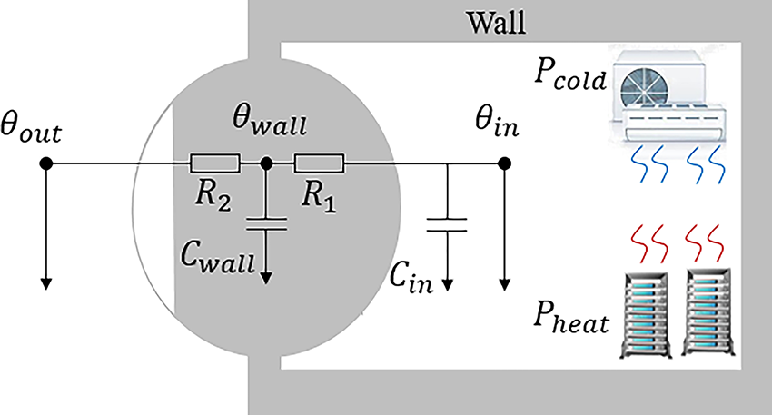
Figure 2: Schematic diagram of the equivalent model of heat transfer process in data center computer room
The energy conservation equation for the indoor air and the walls are constructed as Eqs. (32) and (33).
In the formula, t represents the current time point;
In order to calculate the indoor temperature changes at different discrete time periods within a day, differential equations of Eqs. (32) and (33) are transformed into differential equations, as expressed as Eqs. (34) and (35), with a time step of Δ
Transforming Eqs. (34) and (35) yields Eqs. (36) and (37):
Eqs. (36) and (37) can be used to update the indoor temperature and wall temperature at each time point. Furthermore, according to the practical engineering situation where the variation amplitude of
Regarding the determination of the time step
Combined with the initial indoor temperature
4 Two-Stage Multi-Time Scale Optimization Model for Data Center1
4.1 Two-Stage Multi-Time Scale Scheduling Framework
4.1.1 Day-Ahead and Intra-Day Optimization Scheduling Diagram
The multi-time scale optimization scheduling includes a two-stage day-ahead and intraday rolling optimization scheduling, as illustrated in Fig. 3. The day-ahead scheduling operates on a 24-h optimization scale with 15 min as the time step. Based on the day-ahead forecasts of renewable power and load, the scheduling plan for next 24 h can be formulated with the goal of minimizing the daily operating cost. The intraday rolling optimization scheduling takes 15 min as a rolling round, 60 min as the optimization scale, and 1 min as the time step for each round of optimization. Each round of optimization scheduling is based on 60-min ahead predictions of renewable power and load, aiming to minimize the operating costs of each round of optimization and minimize the fluctuations of exchange power between day-ahead and real-time plans.
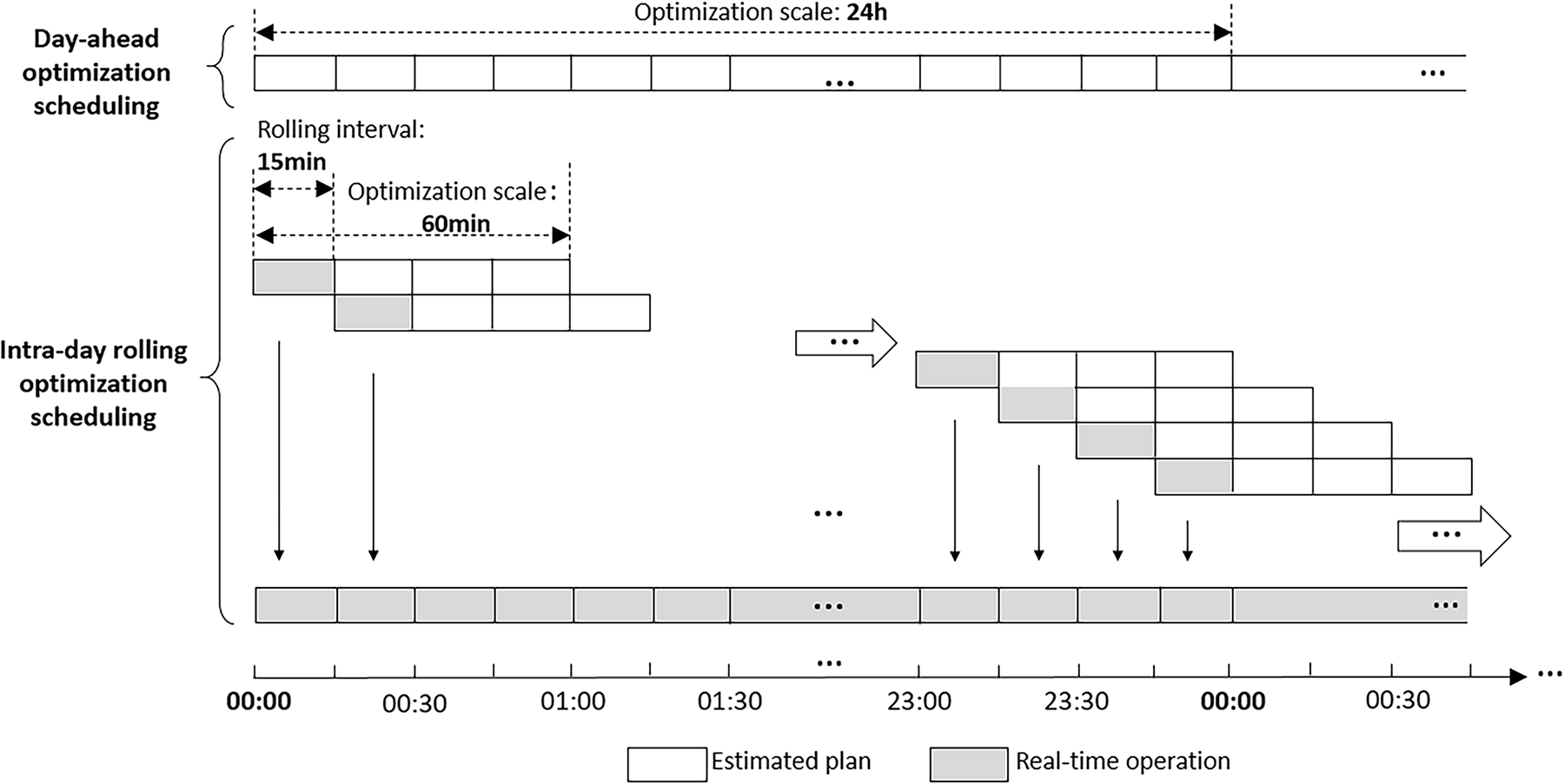
Figure 3: Diagram of the two-stage multi-time scale optimization scheduling framework of data center
4.1.2 Regulation Characteristics at Different Time Scales of Computing Workloads and Refrigeration System
The time step of day-ahead scheduling is generally set as 15 min, which is consistent with sampling interval of power supply and demand. On the one hand, the fluctuations trend of renewable power throughout a day typically exhibit periodic changes. The 15-min interval allows for capturing the primary fluctuation characteristics of wind and PV power, while mitigating the computational burden caused by overly frequent data points. On the other hand, the workloads power consumption is relatively steady throughout the day. Using 15 min as the interval for the measuring of power consumption and as the minimum unit for its movement offers sufficient accuracy to illustrate the load shift mechanism while simplifying data processing. Consequently, the time-shifting model of workloads is suitable to be incorporated into the day-ahead optimization scheduling model. By shifting these workloads along the time axis, the fluctuations of wind and PV power can be offset.
However, the volatilities of wind and PV power at the 1-min level are notably faster and more irregular compared to the daily fluctuations forecasted within a 15-min interval. To address this problem, intra-day real-time scheduling are needed. In this study, the time step in the real-time scheduling stage is 1min, which is consistent with the time interval of the time-variant model of the computer room temperature. Given that refrigeration power serves as the only controllable variable for regulating computer room temperature, by embedding the time-varying temperature model into the intra-day optimization scheduling model, adjusting the refrigeration power every 1 min can effectively cope with the instantaneous fluctuations of wind and PV power. Thus, the refrigeration power can be used as a control variable for intra-day optimization scheduling.
4.2 Day-Ahead Scheduling Optimization Objective
The day-ahead optimization scheduling is designed to minimize operational costs within the dispatching day, expressed as:
The optimization function comprises the net cost of electricity transactions with the main-grid
where
By considering system operation constraints and combining day-ahead forecasts of renewable generation and electricity consumption of fundamental interactive computing workloads, this model can optimize the time shift plan of various delay-tolerant workloads, refrigeration output plan, exchange power plan, wind and PV power utilization plan under the goal of minimizing the operating costs of data center micro-grid during the scheduling day.
4.3 Constraints of Day-Ahead Optimization Scheduling
(1) Constraints of delay-tolerant batch processing workloads
The control variables of the long-running non-interruptible workloads, long-running interruptible workloads, and short-running workloads are
In addition to the above constraints, the other constraints are listed as follows.
(2) Computing power demand balance constraint
This study considers two long-running non interruptible workloads A1 and A2, two long-running interruptible workloads B1 and B2, and short-running workloads C. The total computing power demand of all the workloads at the original state
where
(3) Relation of computing power demand and electricity consumption
where
(4) Indoor temperature constant constraint
If day-ahead forecasted indoor temperature are set to be variable, aligning with the 1-min time step of the time-variant computer room temperature model, day-ahead scheduling would require matching this granularity, which would result in each day-ahead decision variable increasing to 1440 and significantly increasing computational burden. Thus, indoor temperature is fixed at 25°C during day-ahead scheduling. Updates are applied via intraday optimization, which incorporates a refined 1-min temperature variation model.
(5) Refrigeration constraint
The refrigeration power at time point t should meet the upper and lower limits constraints:
In this research,
The relation of
(6) Upper and lower limit of renewable power utilization
The utilized wind and PV power at time point t.
where
(7) Exchange power constraint
The day-ahead planned purchased power and sold power
where
(8) Power supply and demand balance constraint
The total power at supply side of data center equals to the power on demand side:
4.4 Intraday Rolling Optimization Objective
Due to the different time steps of intra-day and day-ahead scheduling, in order to distinguish, the time point in intra-day scheduling is recorded as τ; The time step is recorded as
In the formula, there is:
where
For each round, the control variables are real-time refrigeration power
With reference to Fig. 3, for each round optimization, the first 15-min time period of
4.5 Constraints of Intraday Rolling Optimization
Constraints regarding these variables are described in the following section.
(1) Indoor temperature constraint
For each round, the real-time indoor temperature
The adjacent indoor temperature
where the indoor temperature at the start time
The refrigeration power should satisfy the ramp constraint.
where
(2) Refrigeration power
The refrigeration power should satisfy the ramp constraint.
where
The relationship of
(3) Upper and lower limit of renewable power utilization
Real-time utilized wind and PV power at time
where
(4) Exchange power constraint
Real-time electricity purchase and sale
where
(5) Power supply and demand balance constraint
For each optimization round, the power balance equation constraint at time τ is expressed as:
5 Boundary Conditions and Multi-Time Scale Optimization Scheduling Results
5.1 Boundary Conditions and Parameters of the Data Center
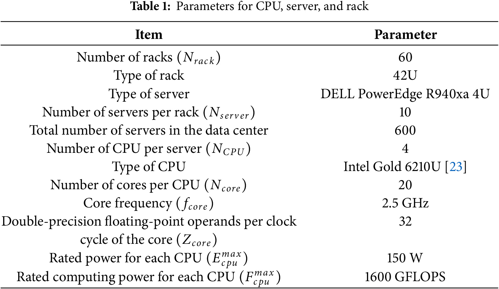
5.1.1 Parameters of the CPU, Server, Rack and Data Center
This study selected a medium-sized data center room in northern China as the example. The data center room occupies an area of 200 m2, with a height of 4 m. The external wall area of the computer room is 240 m2, and the roof area is 200 m2. The data center room is equipped with 60 42U racks, each housing 10 4-way 4U servers. Detailed parameters for the CPU chip, server and rack are outlined in Table 1.
Based on Table 1, in this paper,
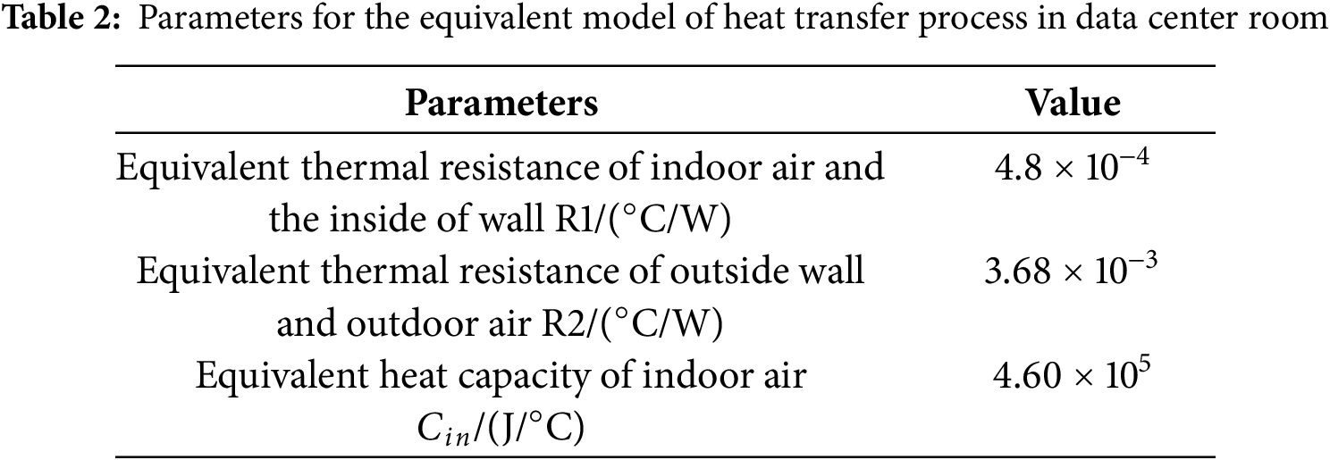
The thermal parameters of the computer room is adapted from literature [26] in accordance with the standards and specifications of data center room construction. The thermal parameters for the equivalent model of heat transfer process in the data center room are given in Table 2.
5.1.2 Parameters of Delay-Sensitive and Delay-Tolerant Workloads
The study considers two long-running non-interruptible workloads (A1 and A2), two long-running interruptible workloads (B1 and B2), and short-running workloads (C). The original computing power demand time series curves for the delay-sensitive interactive workload and delay-tolerant batch processing workloads are depicted in Fig. 4.
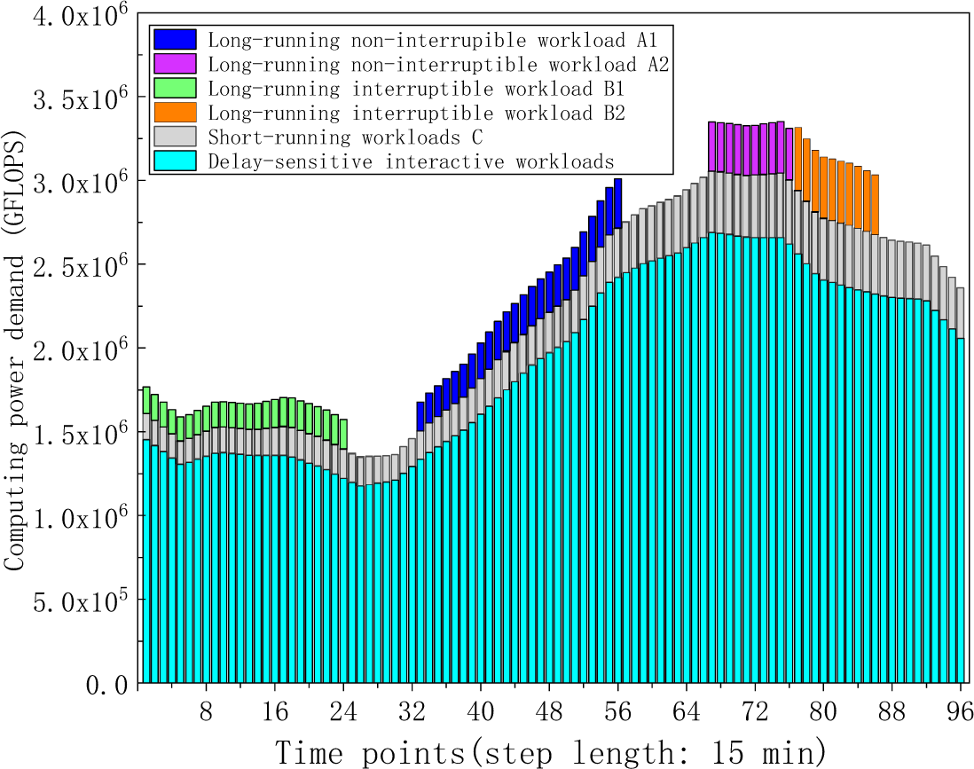
Figure 4: The original computing power demand time series curves of the delay-sensitive and various delay-tolerant workloads
The shifting time range [
5.1.3 Configuration of Refrigeration Power System
The heat load of data center mainly stems from the heat generated by servers and environmental maintenance structure. The rated refrigeration capacity of refrigeration system is determined based on the server equipment power and the area of data center room, as described by the formula:
where
5.1.4 Configuration of Wind and PV Power System
The installed capacity of wind and PV power system, denoted as
In this formula, the average power generation efficiency of renewable energy
Wind and PV power generation data used in the study are sourced from a reliable database [28]. To align with the configured capacities of wind and PV power systems, the data is scaled to generate 24h-ahead forecasts of wind and PV power generation used in this study, as depicted in Fig. 5.
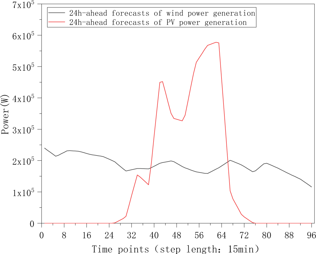
Figure 5: 24 h-ahead forecasts of wind and PV power generation for data center
5.2 Results of Multi-Time Scale Optimization Scheduling
This paper formulates both day-ahead scheduling and intra-day real-time scheduling optimization as Mixed Integer Programming (MIP) optimization problems. The optimization involves continuous variables, e.g., key time-shift parameter variables for various batch computing workloads, and binary variables, e.g., the status of power purchases and sales. Based on the decision variables, equality and inequality constraints, and objective function established in previous sections, the optimization model is solved using Gurobi solver in MATLAB R2024a. The Gurobi solver, widely recognized in academia and industry, employs techniques such as the interior point method, branch and bound method, and cut plane method to find optimal solutions.
This section presents the scheduling results after multi-time scale optimization. Section 5.2.1 details the operational costs and renewable power curtailment results after day-ahead scheduling and verifies its effectiveness by comparing with a simple scheduling scenario. Additionally, it analyzes the comparison of workloads at original status and after scheduling to illustrate the feasibility of the proposed time-shift modelling. Section 5.2.2 reports the operational costs and power exchange volatility results after real-time optimization scheduling. A comparison between the optimization scheduling and a plain real-time scheduling is also conducted to highlight the necessity of incorporating refrigeration regulation in real-time scheduling to cope with the instantaneous power volatility from renewable energy and load demand.
5.2.1 Results after Day-Ahead Optimization Scheduling
To quantitatively verify the effect of considering workloads time-shift, this paper sets up a simple scheduling scenario where the workloads don’t shift over time. In the simple scheduling scenario, the power balance results of utilized wind power
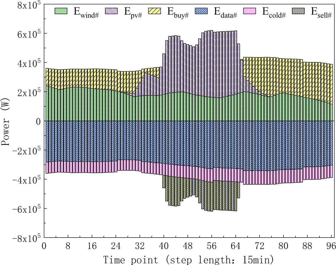
Figure 6: The power balance results in the day-ahead simple scheduling scenario
In the day-ahead optimization scheduling scenario where the time-shiftable workloads are involved, the power balance results of
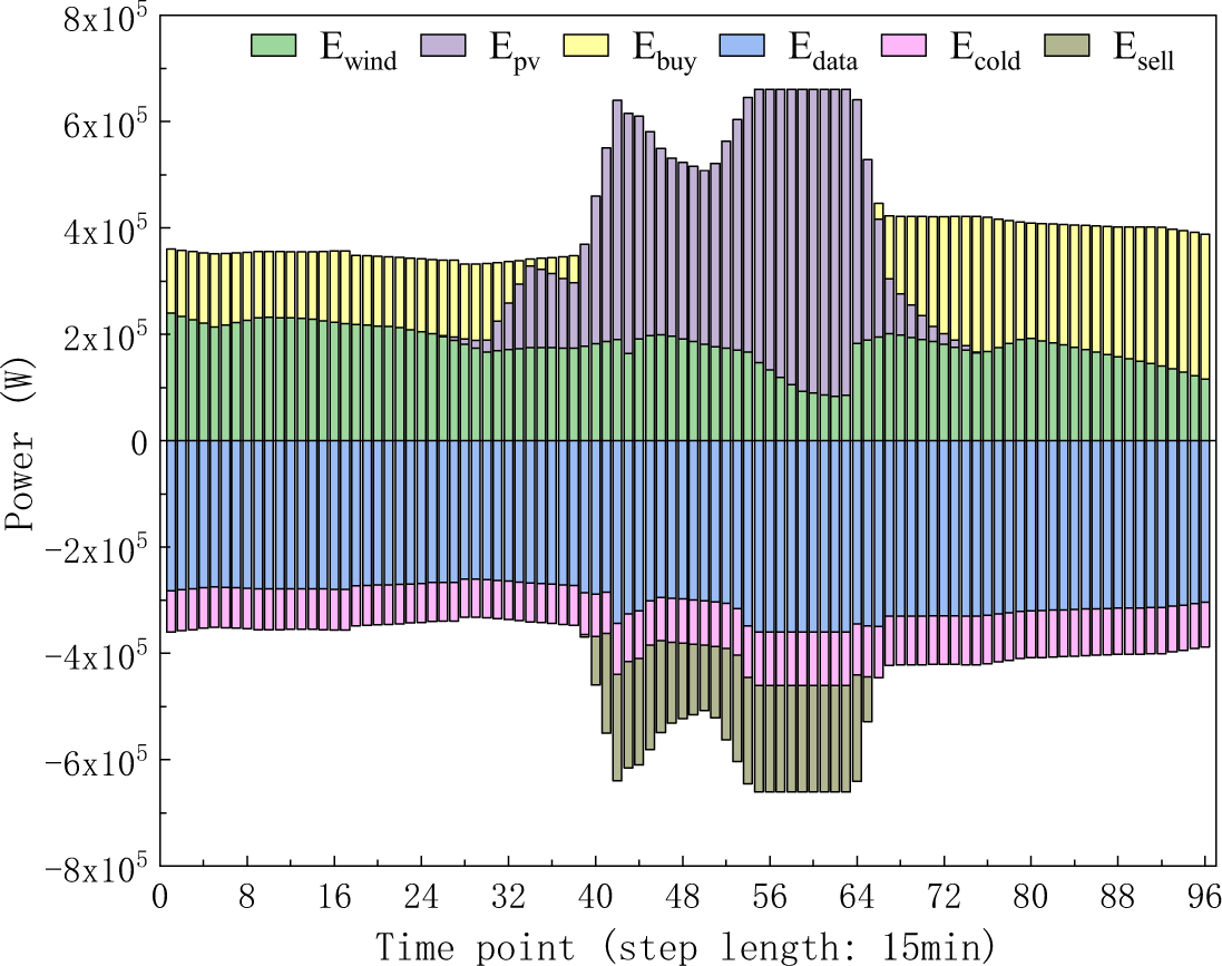
Figure 7: The power balance results in the day-ahead optimization scheduling scenario
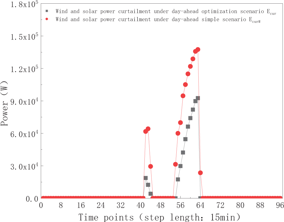
Figure 8: Comparison of wind and PV power curtailment in the day-ahead simple scheduling scenario and the optimization scheduling scenario
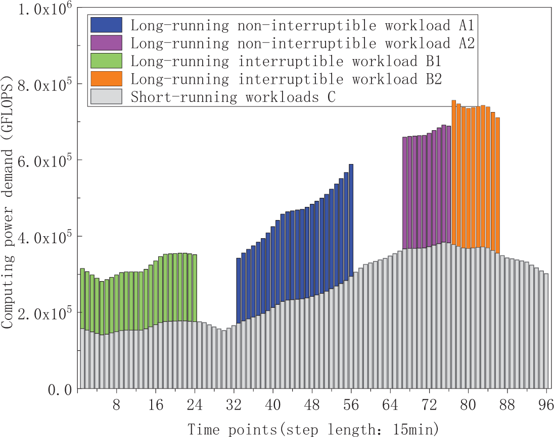
Figure 9: The computing power demand time series of various delay-tolerant workloads at the original state
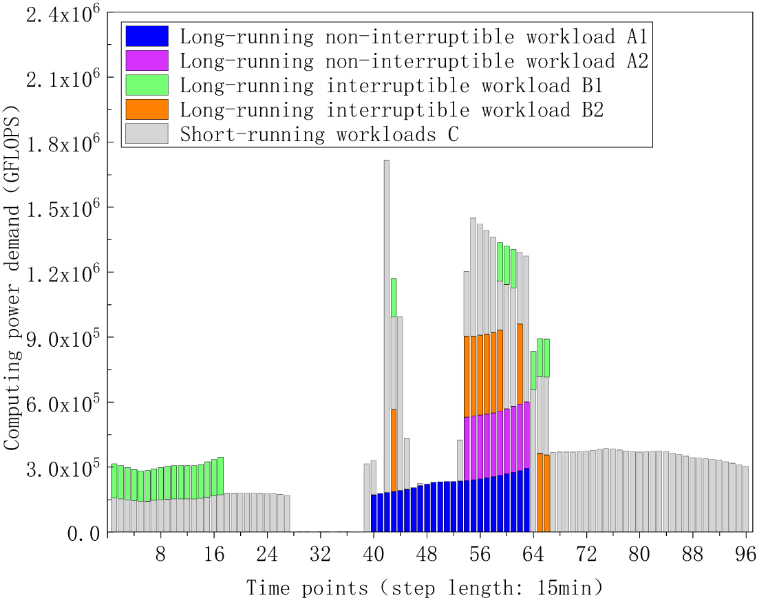
Figure 10: The computing power demand time series of various delay-tolerant workloads after temporal shift
The temporal shift details for the various delay-tolerant workloads are visualized in Figs. 11–15. Specifically, Figs. 11 and 12 display the computing power demand of long-running non-interrupted workloads A1 and A2 before and after shifting. Figs. 13 and 14 illustrate the computing power demand of long-running interruptible workloads B1 and B2, demonstrating that the sequential order of subtasks at different time points and the total computing power demand remain consistent before and after shifting. Additionally, Fig. 15 depicts the computing power demand of short-running workloads C before and after shifting. The results indicate a redistribution of computing power demand as short-running workloads transfer from initial time points to new time points, revealing a decrease in demand during the initial time periods and an increase at the new time periods. The total computing power demand stays unchanged before and after the shifting process. These findings provide evidence supporting the feasibility of workloads’ time shifting, demonstrating the adaptability and efficiency of the workloads scheduling strategy.
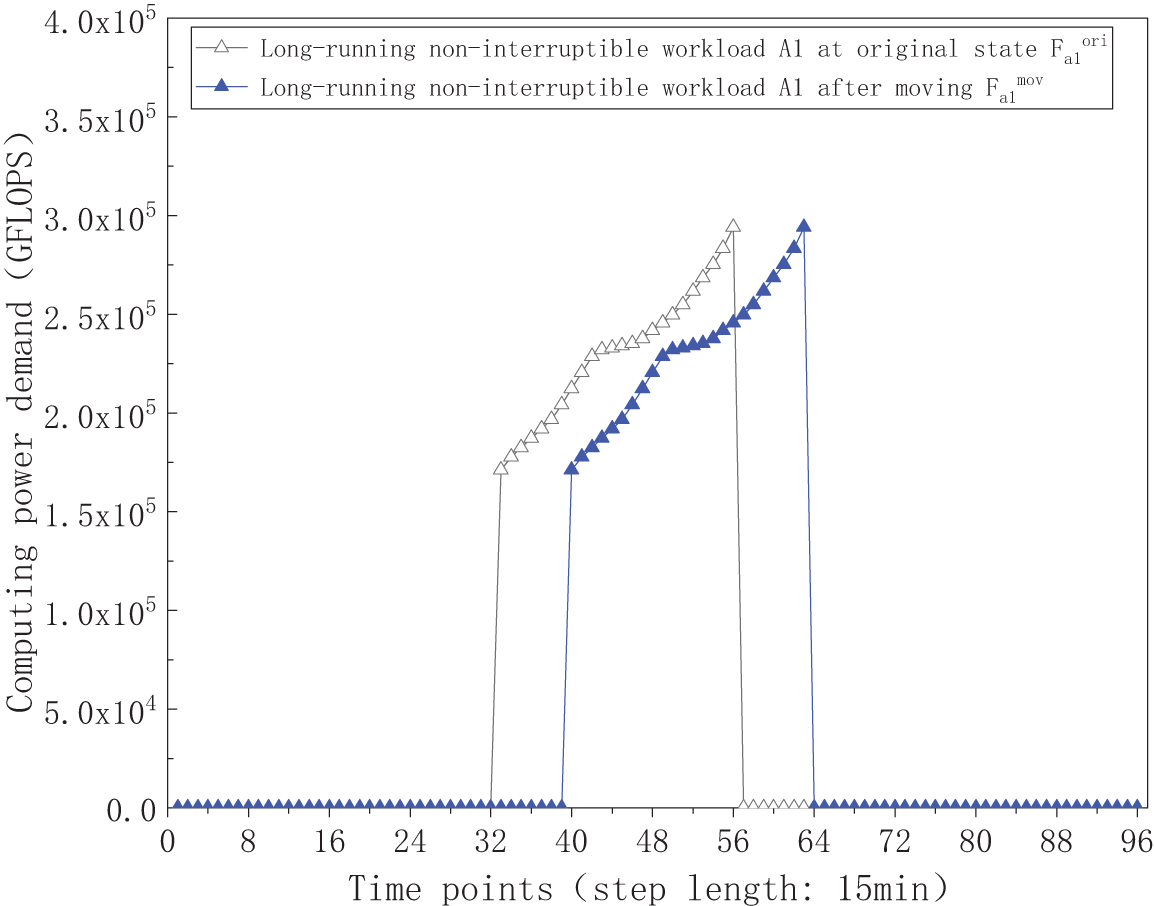
Figure 11: The computing power demand curve of long-running non-interruptible workload A1 at original state and after moving
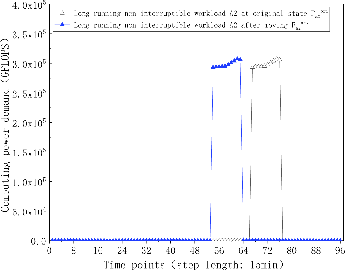
Figure 12: The computing power demand curve of long-running non-interruptible workload A2 at original state and after moving
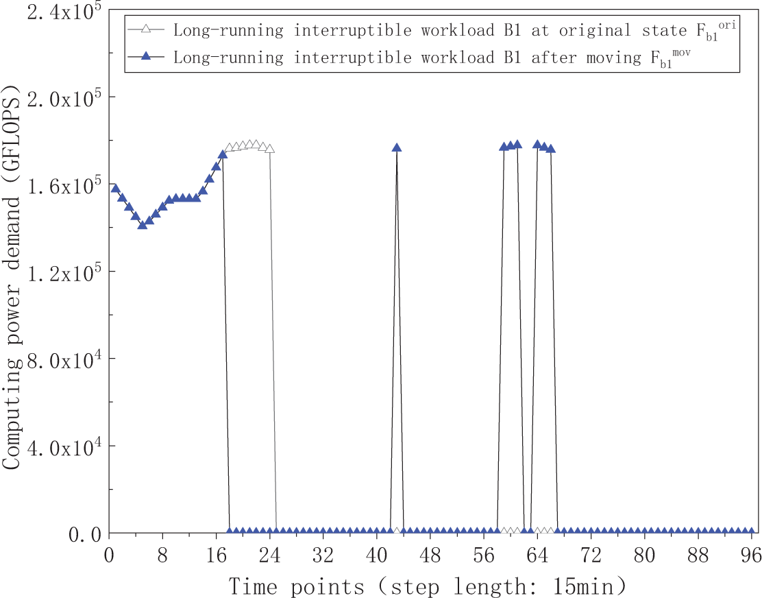
Figure 13: The computing power demand curve of long-running interruptible workload B1 at original state and after moving
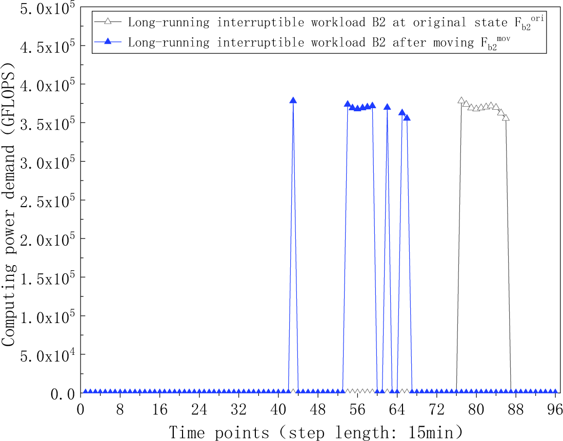
Figure 14: The computing power demand curve of long-running interruptible workload B2 at original state and after moving
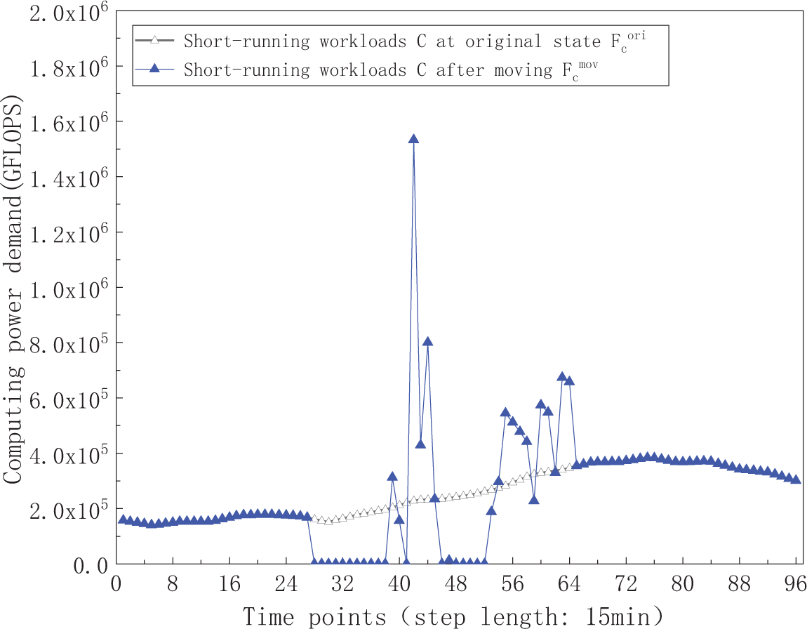
Figure 15: The computing power demand curve of short-running workloads C at original state and after moving
Among the three kinds of workloads, the short-running workloads have a special setting—a penalty coefficient in their time shift model. This paper discusses the rationale behind this setting by comparing the scenarios with and without the penalty coefficient. The time shift result of the various delay-tolerant workloads after the day-ahead optimization scheduling without the penalty coefficient is shown in Fig. 16.
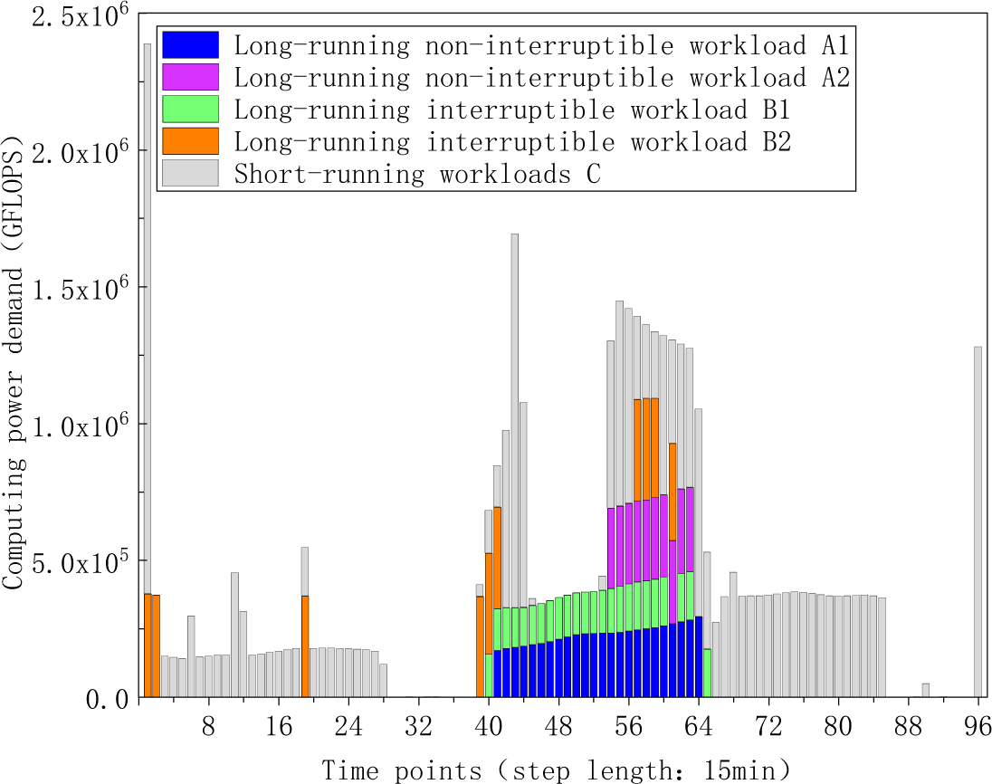
Figure 16: The computing power demand of delay-tolerant workloads after shifting in the scenario without the penalty coefficient setting for short-running workloads
(1) In the scenario with the penalty coefficient setting, most of the short-running workloads C are reallocated to the 43rd–66th time periods, where the surplus wind and solar power is utilized. The reason of this behavior is that, the cost of reducing the wind and PV power sales volume (0.4 + 0.05 = 0.45 ¥/kWh) is lower than the cost of purchasing electricity from other periods (1st–42nd and 67th–96th periods) (0.8 ¥/kWh). For another, this behavior may also lead to electricity revenue (0.6 − 0.05 = 0.55 ¥/kWh) due to reducing penalties for wind and PV power curtailment. Hence, operators are willing to pay lower costs or gain profits by using wind and PV power, rather than purchasing electricity from the main grid.
(2) In the scenario without the penalty coefficient setting, there is still an inflow and aggregation of short-running workloads in the 43rd−66th time periods. Meanwhile, there are also some workloads transferring from the 70th−96th period to the 1st−33rd time period. The mutual transfer of short-running workloads between the 1st−33rd and the 70th−96th time periods is an invalid time shift, since the unit price of power purchase in these two time frames is the same. Thus, the comparison indicates that setting the penalty coefficient for the time-shift model of short-running workloads can avoid invalid movement.
5.2.2 Results after Intra-Day Rolling Optimization
Considering the uncertainty of the day-ahead forecasts of power supply and demand, the day-ahead scheduling plans are updated and corrected by using the intra-day rolling optimization scheduling model. In order to carry out this model, the ultra-short-term 60 min-ahead forecasts of the wind, PV power generation, and server power consumption are needed. According to literature, the 7.5%, 5%, 2.5% mean absolute percentage error of day-ahead forecasts of wind, PV power and server electricity load compared to real-time forecasts are reasonable values [29,30]. Thus, the real-time forecasts of wind power, PV power generation, and server power consumption with a fluctuation ranges of 15%, 10%, and 5% compared to day-ahead forecasts are generated, as shown in Fig. 17a–c. The real-time outdoor temperature is given in Fig. 18.
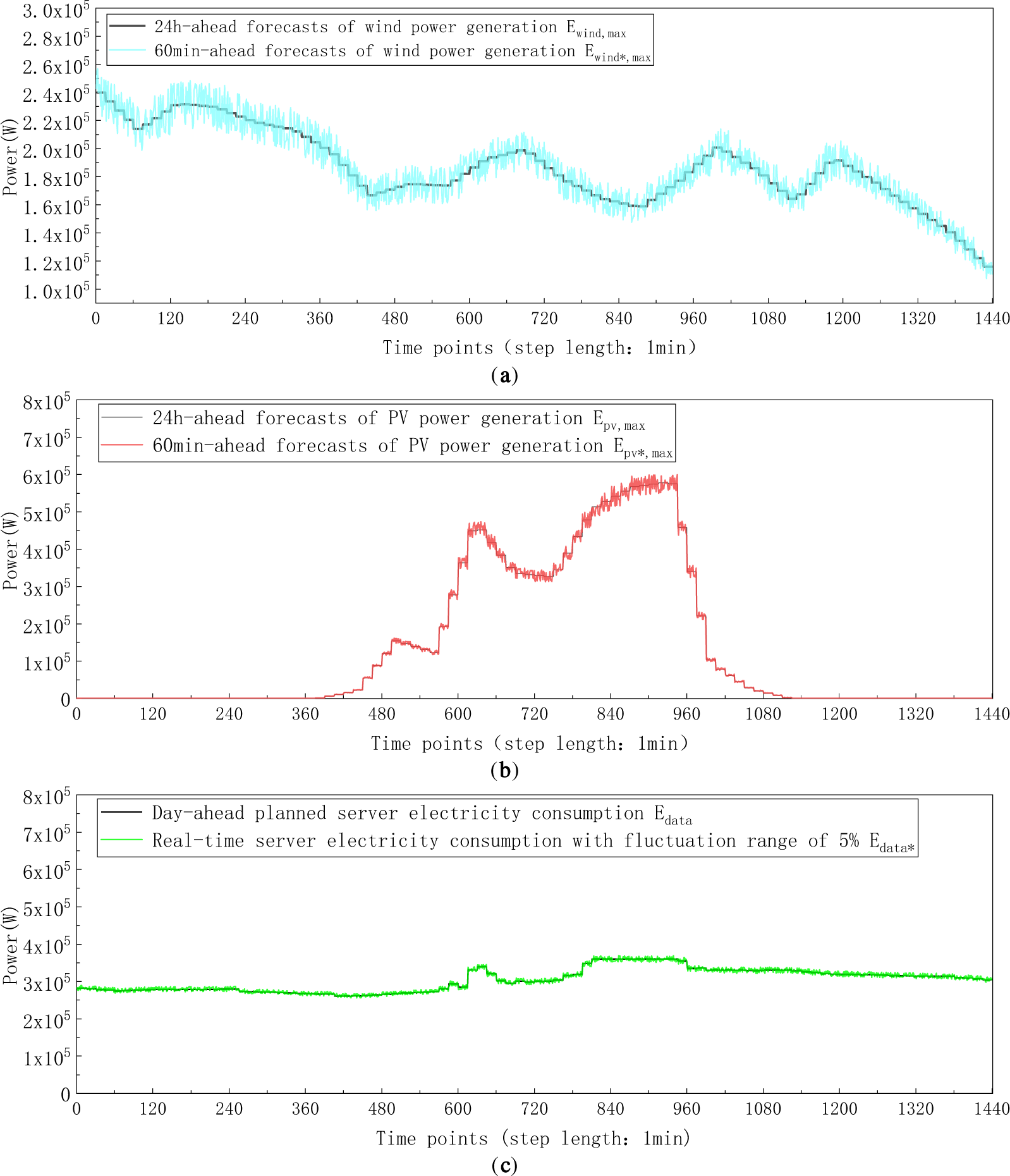
Figure 17: (a–c) Real-time forecasts (plans) and day-ahead forecasts (plans) of wind and PV power generation, and server power consumption. (a) The 60 min-ahead and 24 h-ahead forecasts of wind power generation (step length: 1 min). (b) The 60 min-ahead and 24 h-ahead forecasts of PV power generation (step length: 1 min). (c) Real-time server electricity consumption and day-ahead planned server electricity consumption (step length: 1 min)
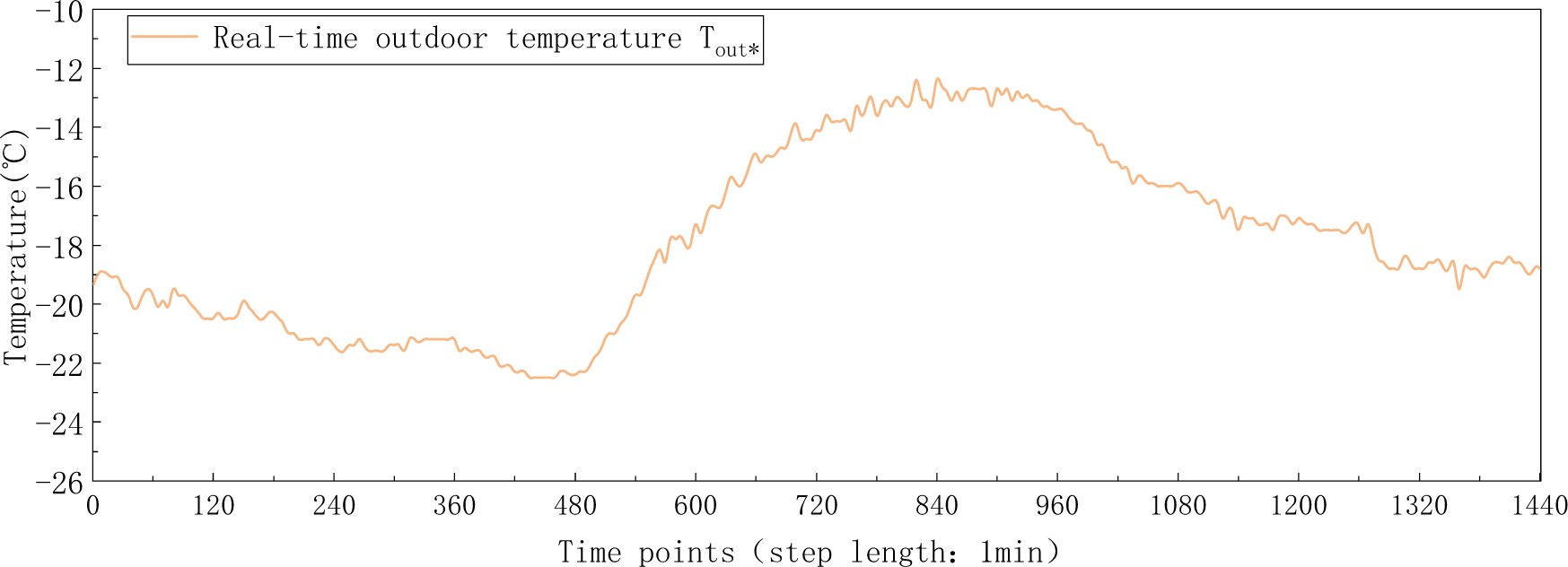
Figure 18: Real-time outdoor temperature (step length: 1 min)
Through the intra-day rolling optimization, the power balance results of utilized wind power
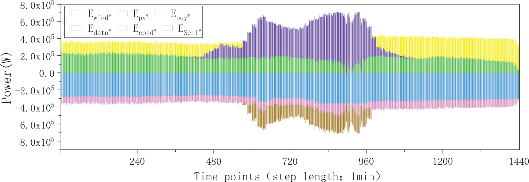
Figure 19: Power supply and demand results after intra-day rolling optimization (step length: l min)
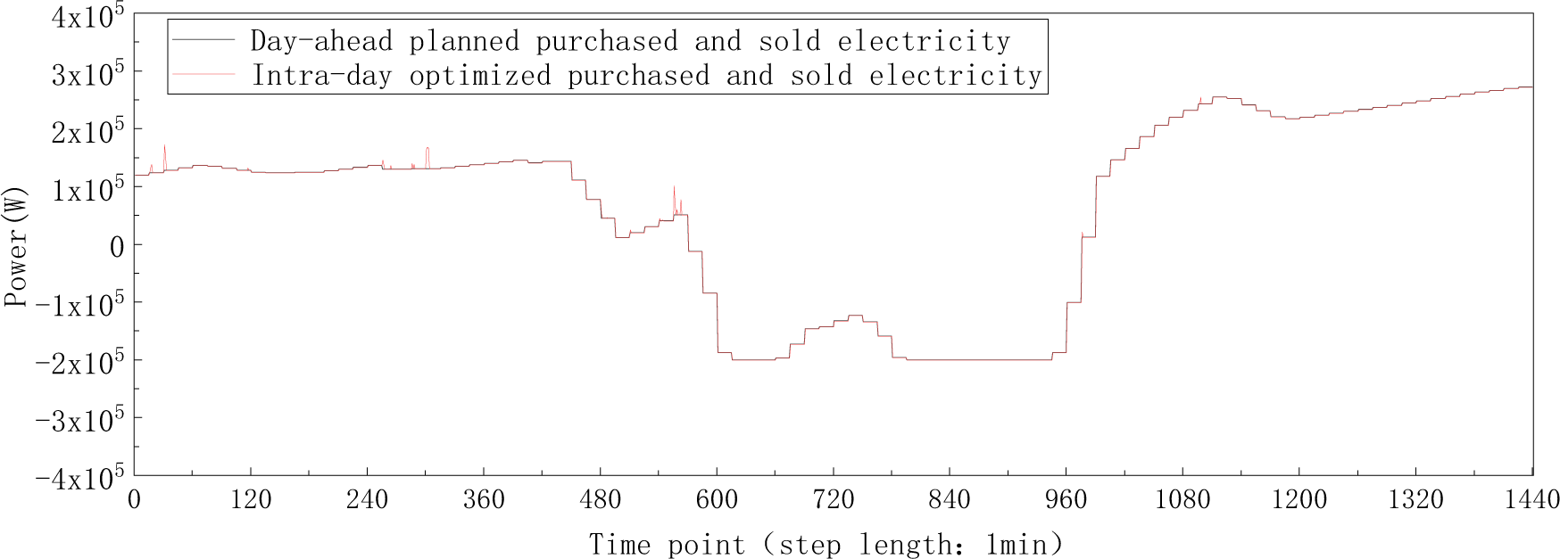
Figure 20: Fluctuation of real-time optimized exchange power relative to the day-ahead planed exchange power (step length: 1 min)
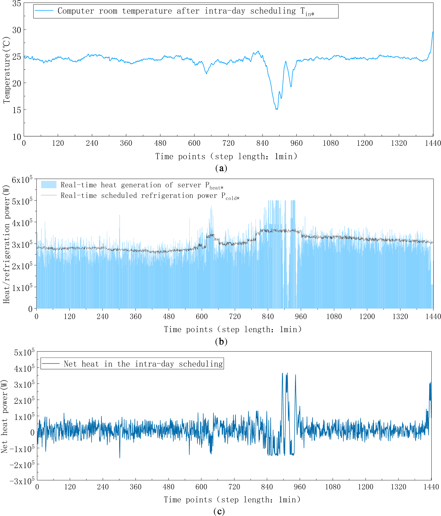
Figure 21: (a–c) Real-time indoor temperature, refrigeration power, heat generation, and net heat after the intra-day rolling optimization (step length: 1 min). (a) The indoor temperature after rolling optimization (step length: 1 min). (b) Real-time beat generation and seheduled refrigeration power (step length: 1 min). (c) Real-time net heat in the intra-day scheduling (step length: l min)
For comparison, this paper sets up a simplified intra-day scheduling scenario that excludes refrigeration modulation flexibility. The calculation determines intra-day power purchases and sales by subtracting 60-min-ahead wind and PV generation forecasts from the combined day-ahead planned server and refrigeration electricity consumption. Fig. 22 depicts the fluctuation of real-time optimized exchange power to day-ahead planned exchange power in this simplified scenario.
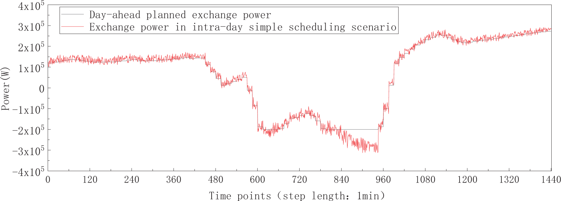
Figure 22: Fluctuation of real-time exchange power relative to day-ahead planned exchange power in the simple intra-day scheduling scenario
After calculation, the exchange power deviation between real-time value and day-ahead plan is 14.92 kW/min, and the daily dispatching cost is ¥2141.4. In comparison to the simple intra-day scheduling scenario, the intra-day optimization scheduling model significantly reduces exchange power fluctuation (by 50 times) and lowers daily operation costs (by 12.9%). This demonstrates the model’s effectiveness in minimizing fluctuations and optimizing system operation economy by leveraging the thermal inertia of the data center computer room and the flexibility of the refrigeration system.
This study investigates the use of delay-tolerant computing workloads and refrigeration systems within data center micro-grid as flexible resources to accommodate volatile renewable generation. A two-stage multi-time scale optimization framework that integrates workload time-shift models into day-ahead scheduling and incorporates refrigeration power as a controllable variable in intra-day dispatch is developed to support green data-center operation. The proposed model is validated on a representative data-center case. Results show that accounting for workload shifting in day-ahead power scheduling reduces daily operating costs by 36.7% and decreases renewable curtailment by 50.5%. Including refrigeration control in intra-day scheduling further improves economic performance and mitigates the impact of renewable uncertainty on exchange-power volatility.
The contribution of this paper includes:
• This work identifies and categorizes three types of delay-tolerant workloads with distinct characteristics. Mathematical models are built to describe their time-shifting mechanisms. These models enable the workload time-shift behavior to be incorporated into renewable-aware power scheduling, allowing computing tasks to actively contribute to low-carbon data-center operation.
• The respective power regulation characteristics of delay-tolerant workloads and data center refrigeration system are analyzed and modelled. Based upon this foundation, a novel multi-time scale power-management framework is established, which achieves the coordination of these two kinds of flexible resources across different time scales to handle renewable power uncertainty.
In future, the deployment of renewable energy in data centers as well as the accelerated expansion of intelligent computation have become an inevitable trend. Further research into scheduling strategies and quantification of power regulation potential of the flexible computing workloads will therefore become essential. The time shift modelling methodology of workloads herein provides a solid foundation and could be applied in these application scenarios. Moreover, the renewable energy uncertainty continues to pose a significant challenge. The two-stage multi-time scale model developed in this study proves to be effective at managing power uncertainty and can be adapted to other green data centers. Overall, this paper contributes a practical management approach that leverages workload shifting and refrigeration flexibility to increase renewable-energy utilization and improve the operational economy of data centers, which provides support to the sector’s green transition.
Acknowledgement: None.
Funding Statement: This work is supported by Science and Technology Standard Project of Guangdong Electric Power Design Institute (ER11301W; ER11811W).
Author Contributions: Luyao Liu: Conceptualization, formal analysis, investigation, methodology, writing—original draft; Xiao Liao: Conceptualization, fund acquisition, project administration, resources; Yiqian Li: Conceptualization, methodology, validation; Shaofeng Zhang: Validation, writing—review & editing. All authors reviewed the results and approved the final version of the manuscript.
Availability of Data and Materials: Data will be made available on request.
Ethics Approval: Not applicable.
Conflicts of Interest: The authors declare no conflicts of interest to report regarding the present study.
Nomenclature
| ASHRAE | American Society of Heating, Refrigerating and Air-Conditioning Engineers |
| A | Long-running non-interruptible workload |
| Original computing power demand time series of the long-running non-interruptible workload | |
| Computing power demand value at the starting node of the long-running continuous workload | |
| Computing power demand value of the long-running continuous workload at the kth time points following the starting node | |
| K | Processing time of the workload execution |
| Time-shift vector of the starting node of long-running continuous workload | |
| Whether the starting node of the long-running non-interruptible workload is located at a certain time point, with a value of 0 or 1 | |
| The time at which the starting node is positioned | |
| The earliest start time point of the long-running non-interruptible workload | |
| The latest start time point of the long-running non-interruptible workload | |
| Computing power demand time series of the long-running non-interruptible workload after shifting | |
| A constructed auxiliary constant matrix, with a dimension of T*T | |
| B | Long-running interruptible workload |
| Original computing power demand time series of long-running interruptible workload | |
| Computing demand value of the 1st subtask of long-running interruptible workload | |
| Computing demand value of the kth subtask of long-running interruptible workload | |
| A constant vector constructed based on values of | |
| Time shift matrix variable of long-running interruptible workload | |
| Whether the kth subtask is moved to time point t, with a value of 0 or 1 | |
| Matrix of time points where subtasks locate after shifting | |
| Time point where each subtask locates after shifting | |
| Computing power demand time series of each subtask after shifting | |
| C | Short-running workloads |
| Original computing power demand time series of short-running workloads | |
| Computing power demand time sequence of the short-running workloads after shift | |
| Computing power demand value of short-running workloads at original status at time point k | |
| Computing power demand value of short-running workloads after shifting at time point t | |
| The amount of computing power demand of short-running workloads that is transferred from the original time point k to another time point of t | |
| The time shift matrix variable of the inflow and outflow computing power demand amount of short-running workloads | |
| A constructed constant matrix with the same dimension as the variable | |
| M | A constant, equal to the peak computing power demand of the short-running workloads. |
| A penalty cost coefficient matrix to prevent invalid shifting | |
| The maximum computing power of the CPU chip | |
| The maximum power consumption of the CPU used in this study | |
| FLOPS | FLoating-point Operations executed Per Second |
| The number of computing cores of the chip | |
| The core frequency | |
| The double-precision floating-point operands per clock cycle of the core | |
| The computing power of the chip | |
| The computing power capacity of the data center using CPU chips | |
| The number of racks in the data center | |
| The number of servers per rack | |
| The number of CPU chips per server | |
| The processor utilization rate | |
| The power of servers when | |
| The power of servers when | |
| The computing power demand of workloads | |
| Equivalent heat capacity of indoor air | |
| Equivalent heat capacity of the wall | |
| R1 | Equivalent thermal resistance of indoor air and the inner side of the wall |
| R2 | Equivalent thermal resistance of the outer wall and outdoor air |
| Indoor temperature at time t | |
| Wall temperature at time t | |
| Outdoor temperature at time t | |
| Heat generation of the servers at time t | |
| Refrigeration power at time t | |
| Mean value of wall temperature | |
| Initial indoor temperature | |
| Net cost of electricity transactions with the main-grid | |
| Penalties for wind and PV power curtailment | |
| Unit electricity purchase price from the main grid | |
| Unit electricity sale price to the main grid | |
| Day-ahead planned purchased electricity power during time period t | |
| Day-ahead planned sold electricity power during time period t | |
| Unit penalty price for wind and PV power curtailment | |
| Day-ahead planned renewable power curtailment in time period t | |
| Duration of time period t | |
| Computing power demand of delay-tolerant workloads A1 | |
| Computing power demand of delay-tolerant workloads A2 | |
| Computing power demand of delay-tolerant workloads B1 | |
| Computing power demand of delay-tolerant workloads B2 | |
| Computing power demand of delay-tolerant workloads C | |
| Computing power demand of delay-tolerant workloads A1 after shift | |
| Computing power demand of delay-tolerant workloads A2 after shift | |
| Computing power demand of delay-tolerant workloads B1 after shift | |
| Computing power demand of delay-tolerant workloads B2 after shift | |
| Computing power demand of delay-tolerant workloads C after shift | |
| Computing power demand of the delay-sensitive workloads | |
| Day-ahead forecasted indoor temperature | |
| Lower limit of refrigeration power | |
| Upper limit of refrigeration power | |
| Day-ahead planned refrigeration electricity power consumption | |
| Day-ahead planned utilized wind power at time point t | |
| Day-ahead planned utilized PV power at time point t | |
| Day-ahead forecasts of maximum wind power generation | |
| Day-ahead forecasts of maximum PV power generation | |
| State of day-ahead power purchase | |
| State of day-ahead power sell | |
| Lower limit of power purchase | |
| Upper limit of power purchase | |
| Lower limit of power sell | |
| Upper limit of power sell | |
| Fluctuation of the purchased and sold power between day-ahead plan and real-time plan for each round | |
| The optimized operation cost for each round | |
| Fluctuation of the purchased and sold power between day-ahead and real-time plan with the minimization of operation costs as the only goal for each round of optimization | |
| The operating cost with the minimization of fluctuation of the purchased and sold power between day-ahead and real-time plan as the only goal for each round of optimization. | |
| Day-ahead planned purchased electricity power at time point | |
| Day-ahead planned sold electricity power at time point | |
| Real-time purchased electricity power at time period | |
| Real-time sold electricity power at time period | |
| Real-time renewable power curtailment at time period | |
| Real-time indoor temperature | |
| Indoor temperature at the start time of intra-day rolling scheduling | |
| Day-ahead planned heat generation of the servers at time | |
| The max fluctuation of indoor temperature within 15 min | |
| The max fluctuation of indoor temperature within 1minute | |
| Real-time refrigeration power at time period | |
| Real-time ramp constraint of refrigeration power | |
| Real-time refrigeration electricity consumption at time period | |
| Real-time planned utilized wind power at time point t | |
| Real-time planned utilized PV power at time point t | |
| 60-min ahead forecasts of maximum wind power generation | |
| 60-min ahead forecasts of maximum PV power generation | |
| State of real-time power purchase | |
| State of real-time power sell | |
| Rated refrigeration capacity of refrigeration system | |
| Corresponding rated electricity consumption of the refrigeration system | |
| The maximum heat generation of the server cluster | |
| The area of the computer room | |
| The empirical coefficient | |
| The installed capacity of wind and PV power system | |
| Average power generation efficiency of renewable energy | |
| Day-ahead planned utilized wind power in the simple scheduling scenario | |
| Day-ahead planned utilized PV power in the simple scheduling scenario | |
| Day-ahead planned purchased power in the simple scheduling scenario | |
| Day-ahead planned server power consumption in the simple scheduling scenario | |
| Day-ahead planned refrigeration electricity consumption in the simple scheduling scenario | |
| Day-ahead planned sold power in the simple scheduling scenario |
1The optimization in this article is without considering cross day load shifting; To isolate the time-shift effect of computing workloads, the energy storage in data center is not considered; The purchase and sale price of electricity in the power grid does not change over time.
2The primary objective of this study is to demonstrate how workload shifting alleviates renewable energy curtailment, which is a core technical contribution. To isolate this mechanism, this paper initially adopt a simplified price assumption, i.e., the purchase and sell price from/to the main grid is a constant, to avoid conflating the curtailment-mitigation effect with price-driven load redistribution. Readers can modify the model’s price settings for further analyses, and the framework remains applicable under these extended scenarios.
References
1. Masanet E, Shehabi A, Lei N, Smith S, Koomey J. Recalibrating global data center energy-use estimates. Science. 2020;367(6481):984–6. doi:10.1126/science.aba3758. [Google Scholar] [PubMed] [CrossRef]
2. IEA (2024Electricity 2024, IEA, Paris. [cited 2025 Aug 06]. Available from: https://www.iea.org/reports/electricity-2024. [Google Scholar]
3. Ni W, Hu X, Du H, Kang Y, Ju Y, Wang Q. CO2 emission-mitigation pathways for China’s data centers. Resourc Conservat Recycl. 2024;202:107383. doi:10.1016/j.resconrec.2023.107383. [Google Scholar] [CrossRef]
4. Patterson D, Gonzalez J, Le Q, Liang C, Munguia L, Rothchild D, et al. Carbon emissions and large neural network training. arXiv:2104.10350. 2021. doi:10.48550/arXiv.2104.10350. [Google Scholar] [CrossRef]
5. Zhang Y, Tang H, Li H, Wang S. Integration and interaction of next-generation AI-focused data centers with smart grids and district energy systems: the state-of-the-art, opportunities and challenges. Renew Sustain Energ Rev. 2025;224:116097. doi:10.1016/j.rser.2025.116097. [Google Scholar] [CrossRef]
6. Cao Y, Zhang S. Facilitating the provision of load flexibility to the power system by data centers: a hybrid research method applied to China. Utilities Policy. 2023;84:101636. doi:10.1016/j.jup.2023.101636. [Google Scholar] [CrossRef]
7. Yang Z, Trivedi A, Liu H, Ni M, Srinivasan D. Two-stage robust optimization strategy for spatially-temporally correlated data centers with data-driven uncertainty sets. Elect Power Syst Res. 2023;221:109443. doi:10.1016/j.epsr.2023.109443. [Google Scholar] [CrossRef]
8. Wang G, Pan C, Wu W, Fang J, Hou X, Liu W. Multi-time scale optimization study of integrated energy system considering dynamic energy hub and dual demand response. Sustain Energy, Grids Netw. 2024;38:101286. doi:10.1016/j.segan.2024.101286. [Google Scholar] [CrossRef]
9. Zhou F, Gu W, Ma G. Advancements in data center cooling systems: from refrigeration to high performance cooling. Energy Build. 2024;320:114634. doi:10.1016/j.enbuild.2024.114634. [Google Scholar] [CrossRef]
10. Chen M, Gao C, Shahidehpour M, Li Z. Incentive-compatible demand response for spatially coupled internet data centers in electricity markets. IEEE Trans Smart Grid. 2021;12(4):3056–69. doi:10.1109/TSG.2021.3053433. [Google Scholar] [CrossRef]
11. Yang T, Jiang H, Hou Y, Geng Y. Carbon management of multi-datacenter based on spatio-temporal task migration. IEEE Trans Cloud Comput. 2021;11(1):1078–90. doi:10.1109/TCC.2021.3130644. [Google Scholar] [CrossRef]
12. Wiesner P, Behnke I, Scheinert D, Gontarska K, Thamsen L. Let’s wait awhile: how temporal workload shifting can reduce carbon emissions in the cloud. In: Proceedings of the 22nd International Middleware Conference; 2021 Dec 6–10; Online. p. 260–72. doi:10.48550/arXiv.2110.13234. [Google Scholar] [CrossRef]
13. Niu T, Hu B, Xie K, Pan C, Jin H, Li C. Spacial coordination between data centers and power system considering uncertainties of both source and load sides. Int J Electr Power Energy Syst. 2021;124(2):106358. doi:10.1016/j.ijepes.2020.106358. [Google Scholar] [CrossRef]
14. Liu Z, Chen Y, Bash C, Wierman A, Gmach D, Wang Z, et al. Renewable and cooling aware workload management for sustainable data centers. ACM SIGMETRICS Perform Eval Rev. 2012;40(1):175–86. doi:10.1145/2318857.2254779. [Google Scholar] [CrossRef]
15. Cupelli L, Schutz T, Jahangiri P, Fuchs M, Monti A, Muller D. Data center control strategy for participation in demand response programs. IEEE Trans Ind Inform. 2018;14(11):5087–99. doi:10.1109/TII.2018.2806889. [Google Scholar] [CrossRef]
16. Kwon S. Ensuring renewable energy utilization with quality of service guarantee for energy-efficient data center operations. Appl Energy. 2020;276:115424. doi:10.1016/j.apenergy.2020.115424. [Google Scholar] [CrossRef]
17. Tang J, Su Z, Wang Y, Zhao M, Liu C, Xu J. Potential analysis of considering the participation of 5G Hongji station air conditioning load in demand response. Power Demand Side Manag. 2022;24(6):77–83. (In Chinese). doi:10.3969/j.issn.1009-1831.2022.06.013. [Google Scholar] [CrossRef]
18. Zhu J, Yang S, Yu L, Jia H. Modeling and temperature control of real-time consumption of renewable energy in data center refrigeration systems. Pow Syst Automat. 2022;46(20):13–22. doi:10.7500/AEPS20220212003. [Google Scholar] [CrossRef]
19. Reiss C, Tumanov A, Ganger GR, Katz RH, Kozuch MA. Heterogeneity and dynamicity of clouds at scale: Google trace analysis. In: Proceedings of the Third ACM Symposium on Cloud Computing; 2012 Oct 14–17; San Jose, CA, USA. p. 1–13. doi:10.1145/2391229.2391236. [Google Scholar] [CrossRef]
20. Lu C, Ye K, Xu G, Xu C-Z, Bai T. Imbalance in the cloud: an analysis on Alibaba cluster trace. In: 2017 IEEE International Conference on Big Data (Big Data). Piscataway, NJ, USA: IEEE; 2018. p. 2884–92. doi:10.1109/BigData.2017.8258257. [Google Scholar] [CrossRef]
21. Beloglazov A, Abawajy J, Buyya R. Energy-aware resource allocation heuristics for efficient management of data centers for cloud computing. Future Gener Comput Syst. 2012;28(5):755–68. doi:10.1016/j.future.2011.04.017. [Google Scholar] [CrossRef]
22. Doyle J, Shorten R, O’mahony D. Stratus: load balancing the cloud for carbon emissions control. IEEE Trans Cloud Comput. 2013;1(1):1. doi:10.1109/TCC.2013.4. [Google Scholar] [CrossRef]
23. Second-generation intelligent Intel ® xeon ® Scalable processor. [cited 2025 Aug 06]. Available from: https://ark.intel.com/content/www/cn/zh/ark/products/series/192283/2nd-generation-intel-xeon-scalable-processors.html. [Google Scholar]
24. ASHRAE 41.I-2020 standard method for temperature measurement. [cited 2025 Aug 06]. Available from: https://www.ashrae.org/. [Google Scholar]
25. Jin C, Bai X, Yang C, Mao W, Xu X. A review of power consumption models of servers in data centers. Appl Energy. 2020;265:114806. doi:10.1016/j.apenergy.2020.114806. [Google Scholar] [CrossRef]
26. Chinese Society of Electrical Engineering. Topic A of the 15th CSEE national college students electrical mathematics modelling competition. [cited 2025 Aug 06]. Available from: http://shumo.neepu.edu.cn. (In Chinese). [Google Scholar]
27. Wang S, Tu R, Chen X, Yang X, Jia K. Thermal performance analyses and optimization of data center centralized-cooling system. Appl Therm Eng. 2023;222:119817. doi:10.1016/j.applthermaleng.2022.119817. [Google Scholar] [CrossRef]
28. European commission Science Hub. [cited 2025 Aug 06]. Available from: https://joint-research-centre.ec.europa.eu/index_en. [Google Scholar]
29. Giebel G, Kariniotakis G. Wind power forecasting—a review of the state of the art. In: Woodhead publishing series in energy, renewable energy forecasting. Oxford, UK: Woodhead Publishing; 2017. p. 59–109. doi:10.1016/B978-0-08-100504-0.00003-2. [Google Scholar] [CrossRef]
30. Liu L, Sun Q, Wennersten R, Chen Z. Day-ahead forecast of photovoltaic power based on a novel stacking ensemble method. IEEE Access. 2023;11:113593–604. doi:10.1109/ACCESS.2023.3323526. [Google Scholar] [CrossRef]
Cite This Article
 Copyright © 2026 The Author(s). Published by Tech Science Press.
This work is licensed under a Creative Commons Attribution 4.0 International License , which permits unrestricted use, distribution, and reproduction in any medium, provided the original work is properly cited.
 Downloads
 Citation Tools