PEMFC Performance Degradation Prediction Based on CNN-BiLSTM with Data Augmentation by an Improved GAN

1  Introduction

Hydrogen energy, as a green and efficient energy carrier, plays a crucial part in the global energy shift. Proton exchange membrane fuel cells (PEMFC) are extremely promising devices for converting hydrogen into electricity, due to their advantages such as elevated energy density, superior conversion efficiency, and moderate operating temperatures [1,2]. However, PEMFC experience irreversible performance degradation during operation, which is caused by both environmental factors and inherent material constraints [3]. Forecasting PEMFC performance degradation is of great significance for cutting down PEMFC maintenance expenses, avoiding malfunctions, and prolonging their lifespan.

PEMFC performance degradation prediction primarily relies on model-driven and data-driven approaches [4,5]. Model-driven approaches typically describe the PEMFC degradation process via mathematical models, followed by identifying, estimating, and updating model parameters to predict the degradation trajectory [6]. These methods rely heavily on precise mathematical models. However, PEMFCs have intricate internal characteristics, which impede the development of accurate models and result in low degradation prediction accuracy [7]. Furthermore, mathematical models exhibit poor generalization under varying design parameters and operating conditions [8], limiting the practical application of model-driven approaches. Data-driven methods eliminate the need to establish mathematical models for PEMFCs. Instead, they leverage statistics, machine learning, and artificial intelligence to mine patterns and features from massive historical experimental data, thereby forecasting performance degradation trends [9–12]. Currently, various data-driven methods have been applied to PEMFC performance degradation prediction, including backpropagation neural networks (BPNN) [13], kernel extreme learning machines (KELM) [14], recurrent neural networks (RNN) [15], long short-term memory networks (LSTM) [16], convolutional neural networks (CNNs) [17], bidirectional long short-term memory (BiLSTM) [18], CNN-LSTM [19], CNN-BiLSTM [20,21], Transformer [22] and others. Among these methods, CNN-BiLSTM achieves a relatively balanced performance in prediction accuracy and computational efficiency. Meanwhile, it can efficiently extract local spatial features and bidirectional temporal information, and has strong processing capabilities for multi-dimensional, spatiotemporally intertwined prediction tasks [23].

Although data-driven methods offer numerous advantages. However, they all require substantial training data to enhance the accuracy of prediction models. In practical operational environments, most data monitoring for PEMFC occurs under normal operating conditions, while monitoring data for faults, failures, and unknown states is scarce [24]. Such imbalanced and insufficient training data will degrade prediction models’ performance [25]. As data mining techniques and artificial intelligence keep advancing, generative adversarial network (GAN) have been widely applied in data analysis and data mining [26]. GAN generate synthetic data that follows a distribution similar to that of the original real data, thereby addressing issues such as insufficient sample size and sample imbalance [27]. Nevertheless, GAN are plagued by issues such as network gradient vanishing and instability. Wasserstein generative adversarial networks (WGANs) were put forward to tackle the issue of gradient vanishing [28], but their use of the fastest gradient descent prevents them from fully extracting more feature information. The WGAN based on gradient penalty (WGAN-GP) was put forward to address the problem of excessively fast gradient descent [29]. However, the distribution of generated samples relies more heavily on the distribution of original samples. In PEMFC prediction, it cannot generate more sample points near the failure criticality, which is unfavorable for the progress of prediction tasks.

In this paper, an improved generative adversarial network (IGAN) with adaptive gradient penalty coefficient is proposed to address the problems of excessively fast gradient descent and insufficient diversity of generated samples. Data generated by IGAN that matches the PEMFC distribution and has high diversity to address insufficient data at failure critical points in performance degradation prediction. A CNN-BiLSTM prediction model is used to forecast PEMFC performance degradation. Experimental results demonstrate that the synthetic data generated by the proposed IGAN exhibits higher quality, and it can fully characterize and enrich the features contained in the original data. With data augmentation, the CNN-BiLSTM model’s prediction accuracy gets enhanced, making it suitable for PEMFC performance degradation prediction tasks.

This paper is structured as follows: Section 2 introduces the relevant theoretical methods and the improvements made in this paper. Section 3 thoroughly describes the structure and core steps of the proposed approach. Section 4 carries out experimental studies to validate the effectiveness of the proposed method and compares it with other techniques. Lastly, Section 5 draws the conclusions.

2  Methodology

2.1 Generative Adversarial Network (GAN)

Motivated by the Nash equilibrium theory, Goodfellow et al. put forward GAN [30]. GAN allows generated data to match the distribution of actual data through adversarial training.

In this paper, GAN is utilized to generate and augment PEMFC data to address the sample imbalance issue. Fig. 1 illustrates the schematic diagram of the GAN model, which mainly consists of two parts: a generator G and a discriminator D. The generator is in charge of creating PEMFC data, while the discriminator is responsible for identifying the authenticity of the data. The specific steps are as follows: random noise z with the distribution Pz is fed into generator G to generate PEMFC data G(z) conforming to the distribution Pg. Generated data G(z) and real data x with the distribution Pdata are combined and input into discriminator D training purposes. During this process, discriminator D is trained to tell if sample data comes from generated data or real data. After that, the trained discriminator is utilized to train generator G, allowing it to create samples more similar to actual fuel cell data. Ultimately, the generator creates data so similar to real data that it can fool the discriminator, whereas the discriminator can no longer tell real and fake data apart. Through this adversarial process, generated data conforming to the distribution of actual PEMFC data is obtained.

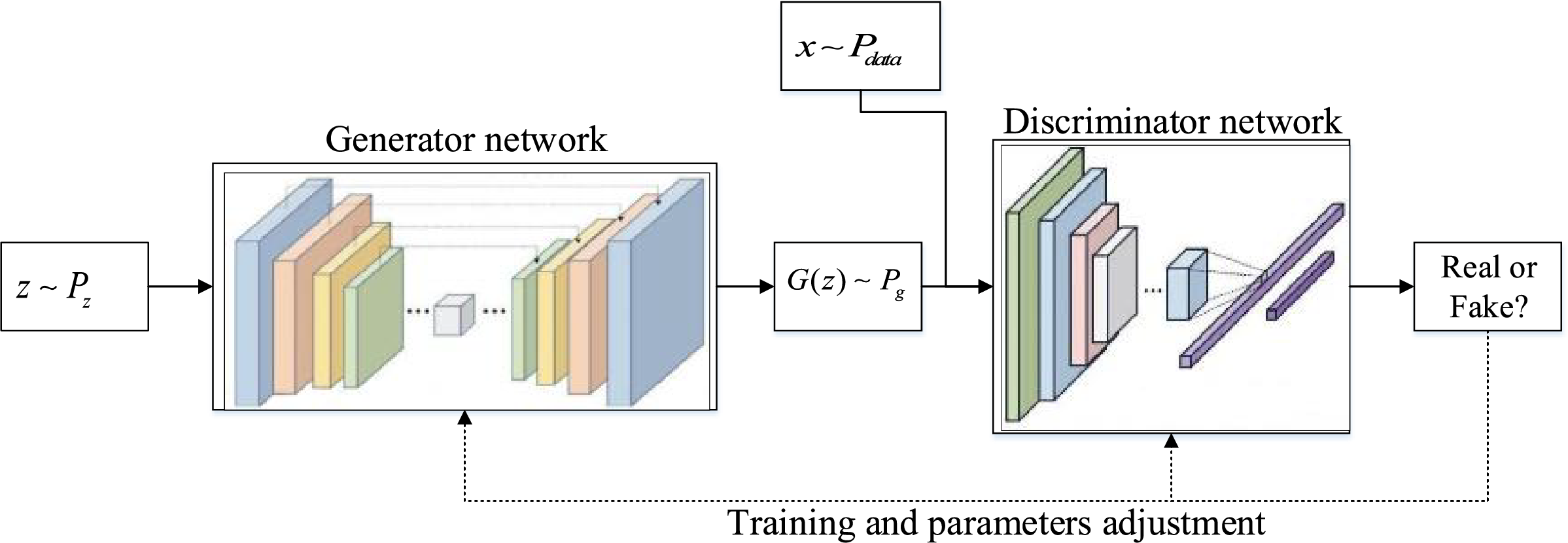
Figure 1: The schematic diagram of the GAN model

Discriminator loss function, generator loss function, and overall optimization objective function of GAN are as follows, respectively:

{L(D)=maxD⁡Ex∼Pdata[log⁡D(x)]+Ez∼Pz[log⁡(1−D(G(z))]L(G)=minG⁡Ez∼Pz[log⁡(1−D(G(z))]minG⁡maxD⁡V(D,G)=Ex∼Pdata[log⁡D(x)]+Ez∼Pg[log⁡(1−D(G(z))],(1)

where, L(D) and LG represent the loss functions of the discriminator and the generator, respectively. minGmaxDV(D,G) denotes the overall objective function of GAN. E[·] denotes the mathematical expectation of the distribution function. D(·) and G(·) serve as the functions of the discriminator and the generator, respectively. Ex∼Pdata[log⁡D(x)] indicates the probability that the discriminator classifies real data as authentic samples, and Ez∼Pg[log⁡(1−D(G(z))] indicates the probability that the discriminator classifies generated samples as fake ones.

Minimizing the divergence between the G(z) and x which can also be represented by the distance between the distributions Pg and Pdata. The objective function can be expressed as:

minGF(D,G)=2DJS(Pg‖Pdata)−2ln⁡(2),(2)

where, DJS(Pg‖Pdata)) denotes the Jensen-Shannon (JS) divergence between Pg and Pdata, which is a metric for gauging the distance between these two distributions. When the discriminator D is trained to its optimal state, the divergence between the two distributions vanishes, and the generator converges to the global minimum.

Following numerous rounds of adversarial training, the generator and discriminator achieve Nash equilibrium. This means that the probability of the discriminator distinguishing between real and fake samples approaches 0.5, indicating that the generator generates data of high quality, which is indistinguishable from real data.

2.2 An Improved GAN

During the adversarial training of GAN, the stochastic mini-batch gradient descent algorithm is employed to update the parameters of the generator and discriminator. However, when there is no overlap between the distribution of real data and that of generated data, the Jensen-Shannon divergence between the two turns into a constant. This gives rise to the issue of gradient vanishing and further causes instability in GAN’s training process. Besides, GAN typically adopts shallow network architectures, which makes it challenging to learn complex data structures and thereby restricts the diversity of samples. To tackle these problems, this paper puts forward an improved GAN (IGAN) strategy as follows.

The smoother Wasserstein distance is utilized to substitute the Jensen-Shannon divergence for gauging the distance between generated samples and real ones. The Wasserstein distance can be expressed as follows:

Dw(Pdata,Pg)=1Ksup‖f‖L≤KEx∼Pdata[f(x)]−Ez∼Pg[f(G(z))],(3)

where, ‖f‖L≤K denotes that the function f is Lipschitz continuous, and its Lipschitz constant does not exceed K. In another words, any two independent variables within the domain satisfy:

|f(x1)−f(x2)|≤K⋅|x1−x2|.(4)

Since it is impossible to solve by traversing all joint distributions, a set of parameters {wi} is used to fit the function f via a neural network to represent all possible functions fw. Thus, the Wasserstein distance can be approximately expressed as:

KDw(Pdata,Pg)=max‖fw‖L≤KEx∼Pdata[fw(x)]−Ez∼Pg[fw(G(z))].(5)

According to Eq. (5), a discriminative network fw with parameters {wi} is constructed, whose final layer excludes a non-linear activation layer. Under the constraint that the parameters {wi} are bounded within a certain range wi∈[−c,c]. Maximizing Dw(Pdata,Pg) to approximate the Wasserstein distance between the real and generated distributions.

After optimizing the discriminator, the generator is then optimized to cut down the Wasserstein distance between the real distribution and the generated one, thus making generated data more similar to real data. The loss functions for the discriminator and the generator can be stated as:

Lw(D)=Ez∼Pg[fw(G(z))]−Ex∼Pdata[fw(x)],(6)

Lw(G)=−Ez∼Pg[fw(G(z))].(7)

The loss functions can indirectly reflect the training status, thereby enhancing the interpretability of the training process.

Although the problem of gradient vanishing can be avoided using the Wasserstein distance, the parameter {wi} must be bounded within a certain range to ensure that the discriminator satisfies Lipschitz continuity. However, the clipping strategy for parameters {wi} has a significant negative impact on optimization: weights are often clipped to c or −c, causing the neural network to adopt the simplest method to achieve the fastest gradient descent. In this case, the network can only learn simple features, which limits the quality of generated samples. To address this issue, this study introduces gradient penalty (GP) into discriminator D’s loss function to add gradient constraints on input samples, thereby reducing the update rate of weights and ensuring that weight changes remain within a reasonable range. The gradient penalty method is stated as follows:

GP=βEx^∼Px^[(‖∇x^fw(x^)‖2−1)2],(8)

where, β denotes the penalty coefficient, and x^ represents the linear interpolation between generated samples and real samples, which can be described as:

x^=ηx+(1−η)G(z),(9)

where, η is uniformly distributed over the interval [0, 1].

In PEMFC data, the sample size corresponding to normal states is typically large, while that corresponding to abnormal states is small. During GAN training, the distribution of gradient norms ‖∇x^fw(x^)‖2 dynamically changes under the influence of factors such as data distribution and the generator. The use of a fixed penalty coefficient β may lead to excessively strong or weak constraints. Excessively strong constraints will make the generator more inclined to generate “normal state data” with a large sample size, while excessively weak constraints will result in training collapse. To address this issue, we apply the adjustment mechanism of the proportional controller to the regulation of the penalty coefficient, as detailed below:

βt+1=(χ⋅(μt−1)+1)⋅βt,(10)

where, βt denotes the penalty coefficient at the t-th training iteration, μt represents the moving average of gradient norms at the t-th iteration, and χ is the adjustment rate. By continuously correcting the error, the gradient norms are stabilized around the target value, thus approximately satisfying the 1-Lipschitz condition.

The discriminator’s objective loss function is updated in the following way:

LwGP(D)=−Ex∼Pdata[fw(x)]+Ez∼Pg[fw(G(z))]+βtEx^∼Px^[(‖∇x^fw(x^)‖2−1)2].(11)

IGAN can achieve uniform distribution of gradients during the training process, enabling it to better extract features and boost the stability of training.

2.3 CNN-BiLSTM

The CNN can alternately use convolutional layers and pooling layers through local connectivity and weight sharing, enabling it to obtain effective representations from original signals, automatically capture local data features, and build dense, comprehensive feature vectors [31]. BiLSTM is made up of two separate LSTM structures, conducting forward and backward feature learning on the input sequence [32]. This lets it thoroughly capture the past and future info of the input time-series data, efficiently enhance the model’s capacity to capture dependencies, and boost prediction accuracy. This paper uses the CNN-BiLSTM hybrid model as the predictor for fuel cell performance degradation, with its structure depicted in Fig. 2.

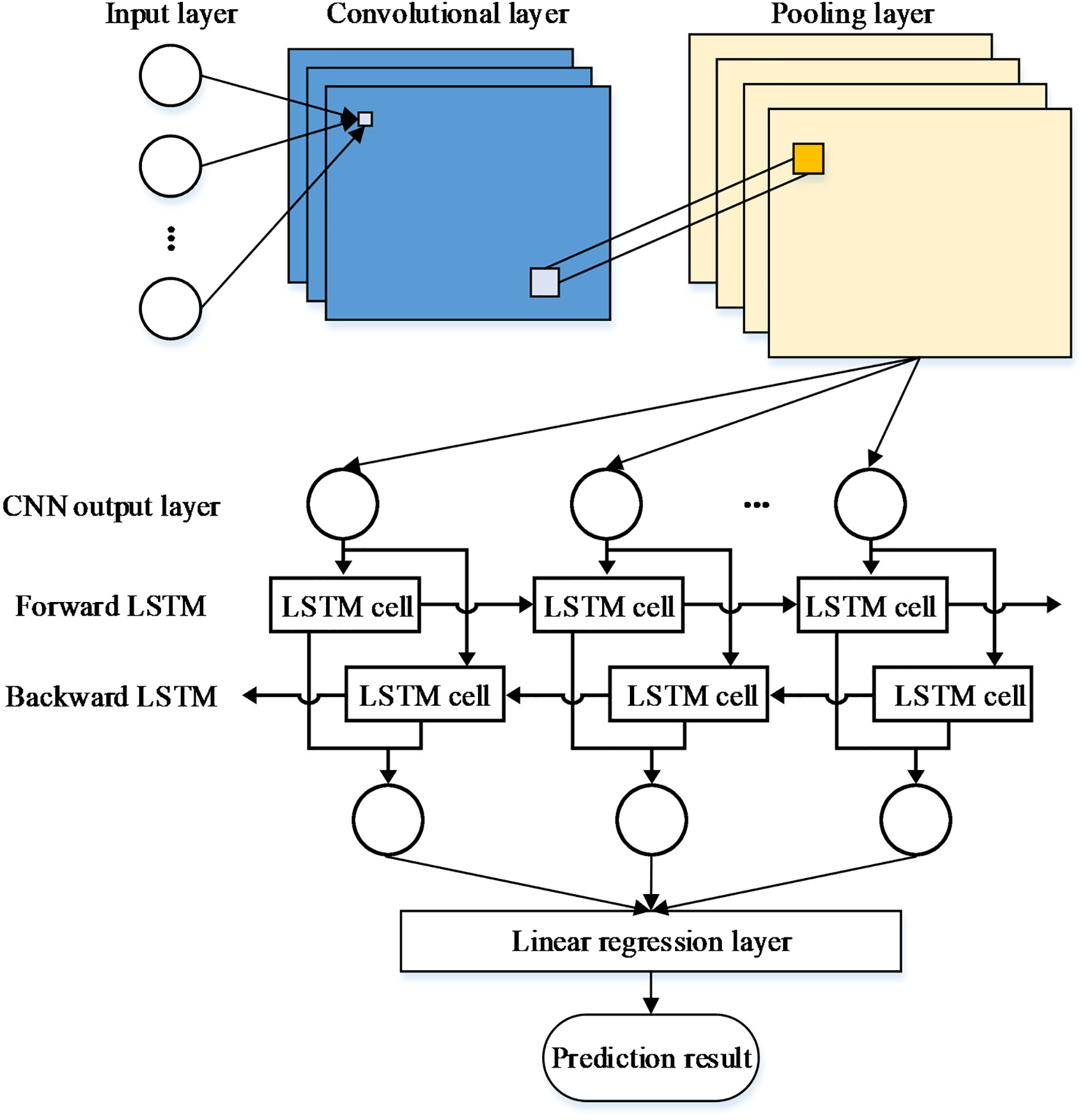
Figure 2: The model structure of CNN-BiLSTM

The CNN consists of an input layer, convolutional layers, pooling layers, fully connected layers, and an output layer. The convolutional layer acts as the core part of the whole CNN, where the convolutional kernel is utilized to filter and capture local features from the data, which is expressed as follows:

Cj=fR(∑A∗W+b),(12)

where, Cj denotes the convolutional kernel, fR represents the non-linear ReLU activation function, A is the input, W denotes the weight, ∗ represents the convolution operator, and b is the bias.

Pooling layers serve to compress data and eliminate redundant information to avoid overfitting. This paper adopts max-pooling layers. After pooling, features are integrated in fully connected layers to obtain the CNN’s output data.

BiLSTM consists of forward and backward LSTM units. Each LSTM cell has a forget gate Ft, an input gate It, and an output gate Ot, with their structure displayed in Fig. 3.

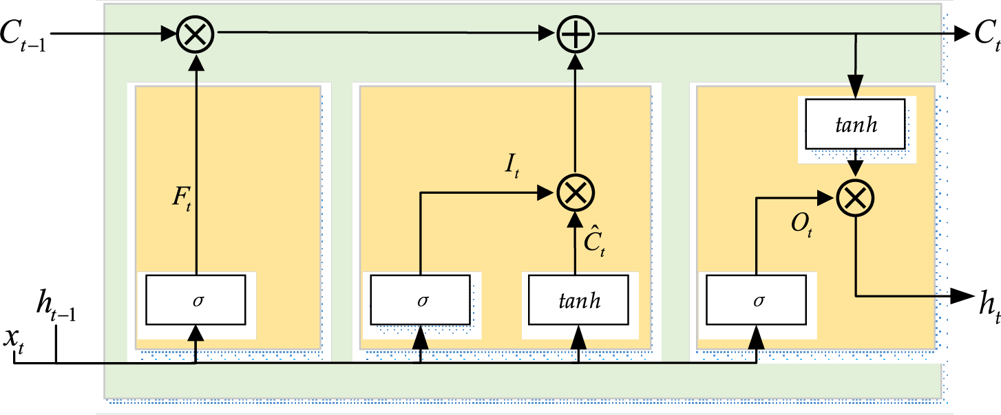
Figure 3: The structure of BiLSTM

The input gate It regulates the state of the current input in the memory cell, the forget gate Ft screens the handling outcomes of the previous memory cell to decide whether to keep them; and the output gate Ot governs the output state of the memory cell. The network computation procedure of LSTM can be stated as follows:

Ft=σ(Wf[xt,ht−1]+bf),(13)

It=σ(Wi[xt,ht−1]+bi),(14)

C^t=tanh⁡(Wc[xt,ht−1]+bc),(15)

Ct=Ft⊗Ct−1+It⊗C^t,(16)

Ot=σ(Wo[xt,ht−1]+bo),(17)

ht=Ot⊗tanh⁡(Ct),(18)

where, C^t signifies the current cell state, Ct−1 stands for the previous cell state, Ct denotes the updated cell state, ht represents the LSTM’s hidden layer, ht−1 is the previous hidden layer, σ is the Sigmoid activation function, tanh is the hyperbolic tangent activation function, xt is the current input. Wf, Wi, Wc, and Wo are the gate-corresponding weight coefficients. bf, bi, bc, and bo are the respective gate biases.

In BiLSTM, the hidden layer ht at each level is formed by the combination of the forward hidden layer and the backward hidden layer, and can be expressed as:

ht=h→t⊕h←t,(19)

where, h→t stands for the forward LSTM’s hidden layer, h←t denotes the backward LSTM’s hidden layer, ⊕ indicates the element-wise sum of the forward output component and the backward output component.

In this paper, the CNN employs 2 convolutional layers to extract data features, and 1 pooling layer to filter the extracted data features. Subsequently, the pooled feature data are used for prediction via BiLSTM. The specific parameter settings are as follows: The two convolutional layers of the CNN have 32 and 64 kernels, respectively, and employ the ReLU activation function. The BiLSTM contains 64 memory units in the unidirectional mode, with a total of 128 memory units in the bidirectional mode. The fully connected layer employs the ReLU activation function. For the CNN-BiLSTM model, the number of training epochs is set to 300, the learning rate is 0.001, and the dropout rate is 0.2.

3  The Structure and Key Steps of the Proposed Method

In this paper, IGAN is put forward to augment PEMFC data, so as to balance data distribution and fully reflect PEMFC’s degradation characteristics. Meanwhile, CNN-BiLSTM is utilized to predict PEMFC’s performance degradation. To clearly illustrate steps and architecture of the proposed approach, the framework diagram is presented in Fig. 4. Main steps of this method are outlined as follows:

Step 1: Abnormal data in the original dataset is removed, and massive redundant data within the original data is eliminated via data reconstruction. The quality of the data is improved via moving average processing. Variables highly correlated with PEMFC performance are selected to predict performance degradation.

Step 2: The IGAN algorithm proposed in this paper is employed to generate synthetic data consistent with the distribution of real PEMFC data. Real data and synthetic data are merged to form augmented data, so as to improve the balance and diversity of the data.

Step 3: The CNN-BiLSTM model is used to predict the stack voltage of PEMFC, and performance degradation of PEMFC is analyzed based on the prediction results.

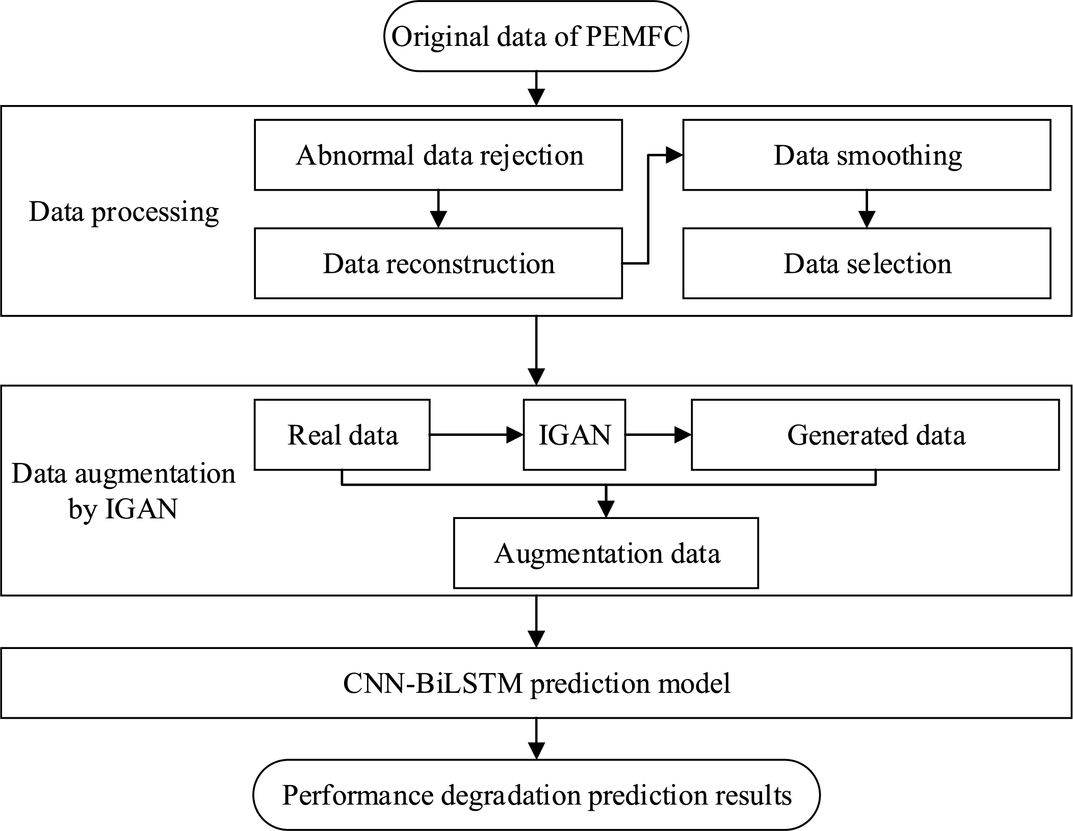
Figure 4: The framework diagram of the proposed prediction model

4  Experimental Study

4.1 Data Description and Data Processing

An experimental dataset provided by the French Fuel Cell Laboratory (FCLAB) is used. A PEMFC was tested for more than 1000 h on the platform. The fuel cell stack consists of 5 single cells with a rated power of 1 kW, a single-cell active area of 100 cm2, the rated current density of 0.70 A/cm2, and a maximum current density of 1 A/cm2 [33]. The steady-state dataset FC1 was obtained under the condition that the operating current density was constant at 0.7 A/cm2, while the quasi-dynamic dataset FC2 was acquired when the operating current density varied within the range of (0.7 ± 0.07) A/cm2. The feature parameters in the dataset include time, single-cell voltage, stack voltage, current, as well as the temperature, humidity, flow rate, and pressure of the reactant gas at the inlet and outlet. Observed from the original data, the stack voltage shows a significant decrease or fluctuation over time. Therefore, this paper selects the stack voltage as the indicator of PEMFC performance degradation and conducts prediction on it.

During data collection, the data is susceptible to external interference, resulting in a large amount of noise and abnormal data points in the original data. Meanwhile, there are numerous redundant samples in the data, which can adversely affect the prediction results and increase the computational load of prediction. Therefore, preprocessing of the original data is required. This paper employs the stationary wavelet transform (SWT) algorithm to perform smoothing and denoising on the original data, and reconstructs the data at a time interval of 0.5 h. After reconstruction, FC1 contains 2308 data samples and FC2 contains 2041 data samples. The comparison between the stack voltage after smoothing and reconstruction and the original stack voltage is shown in Fig. 5. As observed from the figure, the processed data not only preserves the primary trend of the original data but also successfully removes noise and abnormal data points.

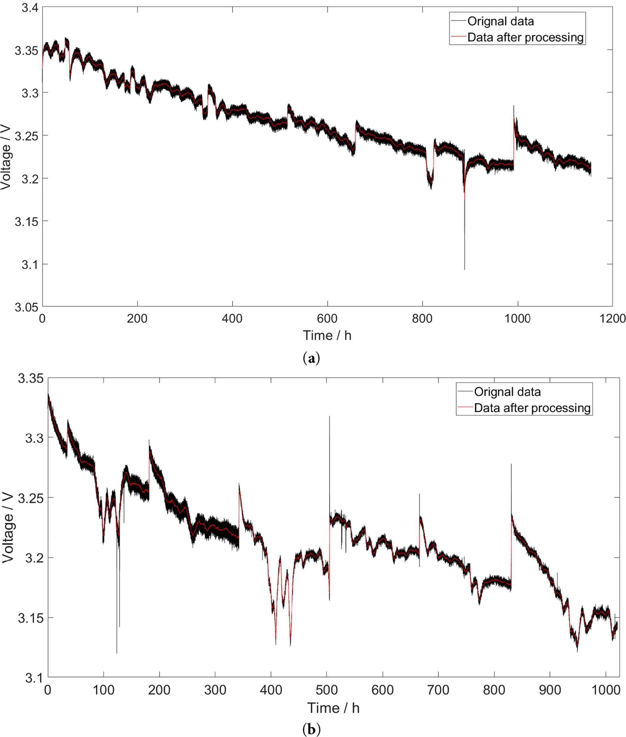
Figure 5: The original data and processed data of stack voltage. (a) FC1; (b) FC2

The sampled data contains a large number of variables, but not every variable has a predictive effect on battery performance degradation. Using irrelevant variables for prediction not only increases the computational complexity of the model but also affects the prediction accuracy of the model. Therefore, this paper adopts the principal component analysis (PCA) method to analyze high-dimensional data, the explained variance and cumulative explained variance is shown in Fig. 6.

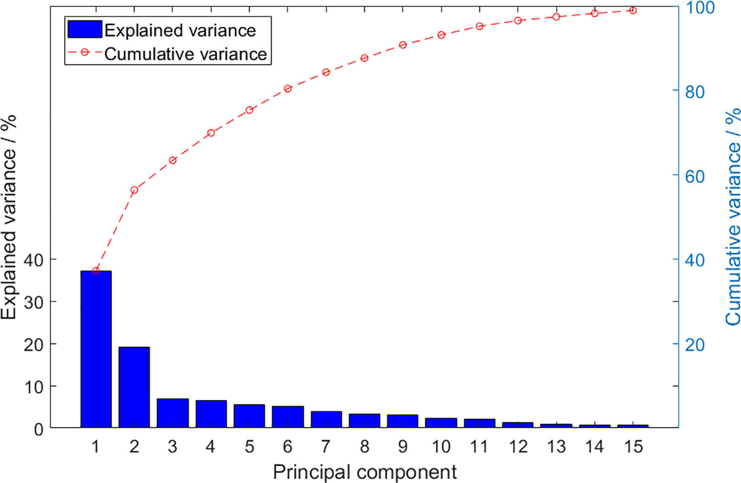
Figure 6: The explained variance and cumulative explained variance of PCA

The cumulative explained variance of the first nine principal components exceeds 90%. The loading matrix of these nine principal components is used to calculate the weighted sum of each variable, so as to measure the importance of each original variable. Variables with larger weighted sums are selected as input variables. Finally, time, stack voltage, 5 single-cell voltages, current, current density, inlet air and hydrogen temperatures, along with outlet air and hydrogen temperatures, are chosen as input variables for the prediction model.

4.2 Augmented Data by IGAN

In this paper, 60% of PEMFC data is chosen as training data for the proposed predictor, with 40% used as validation data. To verify the role of the proposed IGAN in data augmentation, the real PEMFC training data is augmented. Among them, FC1 contains 1384 real samples and FC2 contains 1224 real samples. GAN and IGAN are used respectively to generate samples. To verify quality of synthetic samples produced here, t-distributed stochastic neighbor embedding (t-SNE) dimensionality reduction is performed on both real samples and generated samples, and visualization is used to show the distribution of different datasets, depicted in Fig. 7.

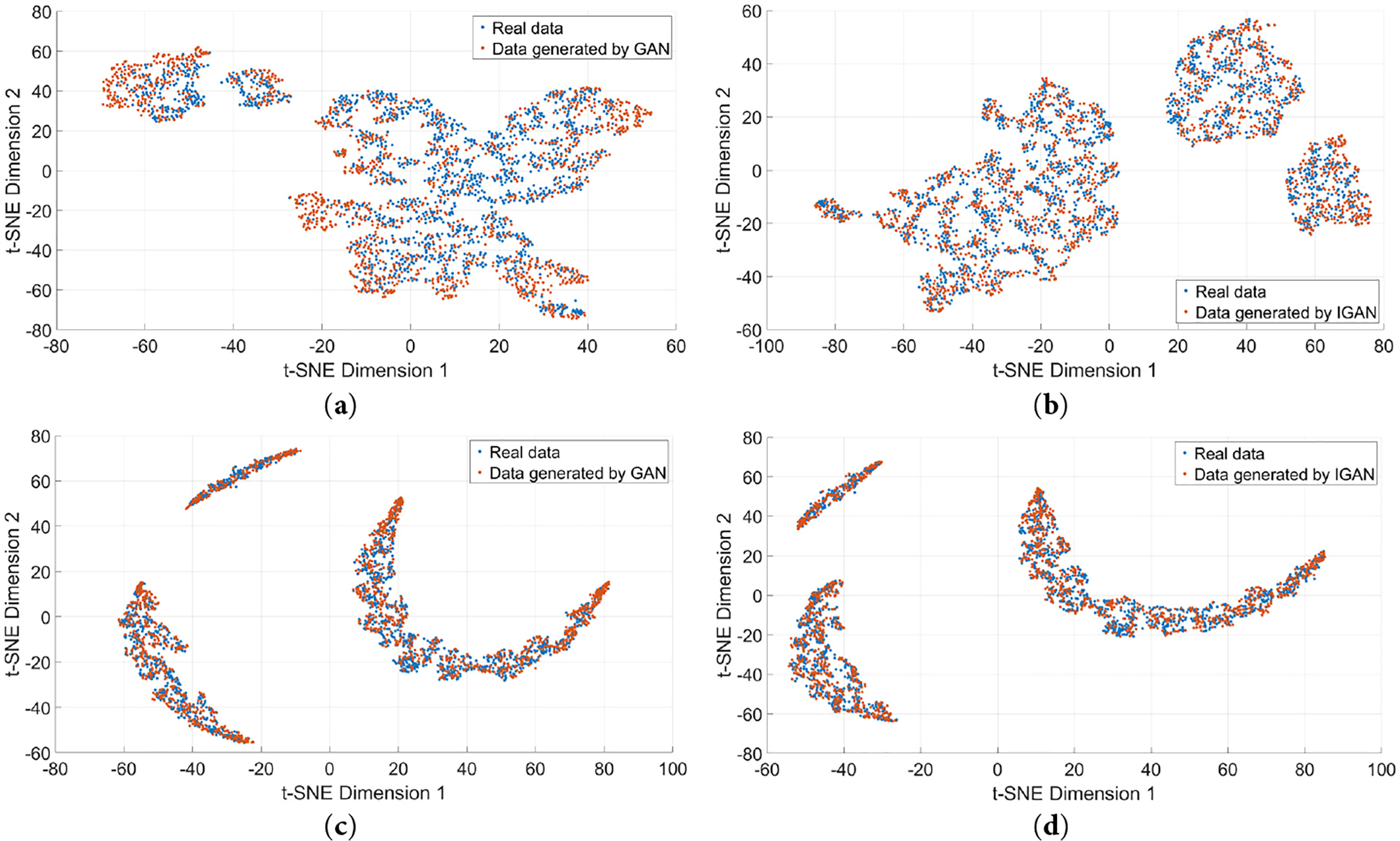
Figure 7: The t-SNE view of the distribution of reduced features of real data and generated data. (a) Data augmentation by GAN of FC1; (b) Data augmentation by IGAN of FC1; (c) Data augmentation by GAN of FC2; (d) Data augmentation by IGAN of FC2

Fig. 7 shows that the distribution of generated data points is highly similar to that of real data points, verifying that the data augmentation approach can acquire data with features akin to the real data. It can be further observed that the distribution of GAN shows partial over-concentration, which is attributed to the problem of insufficient features in generated data caused by gradient vanishing. In contrast, the distribution of IGAN is more uniform than that of GAN, implying the IGAN proposed herein has better performance and the generated data has higher quality.

To quantify the effect of data augmentation more clearly, the voltage decay interval of the FC1 stack is used to measure the sample distribution before and after data augmentation, as shown in Table 1.

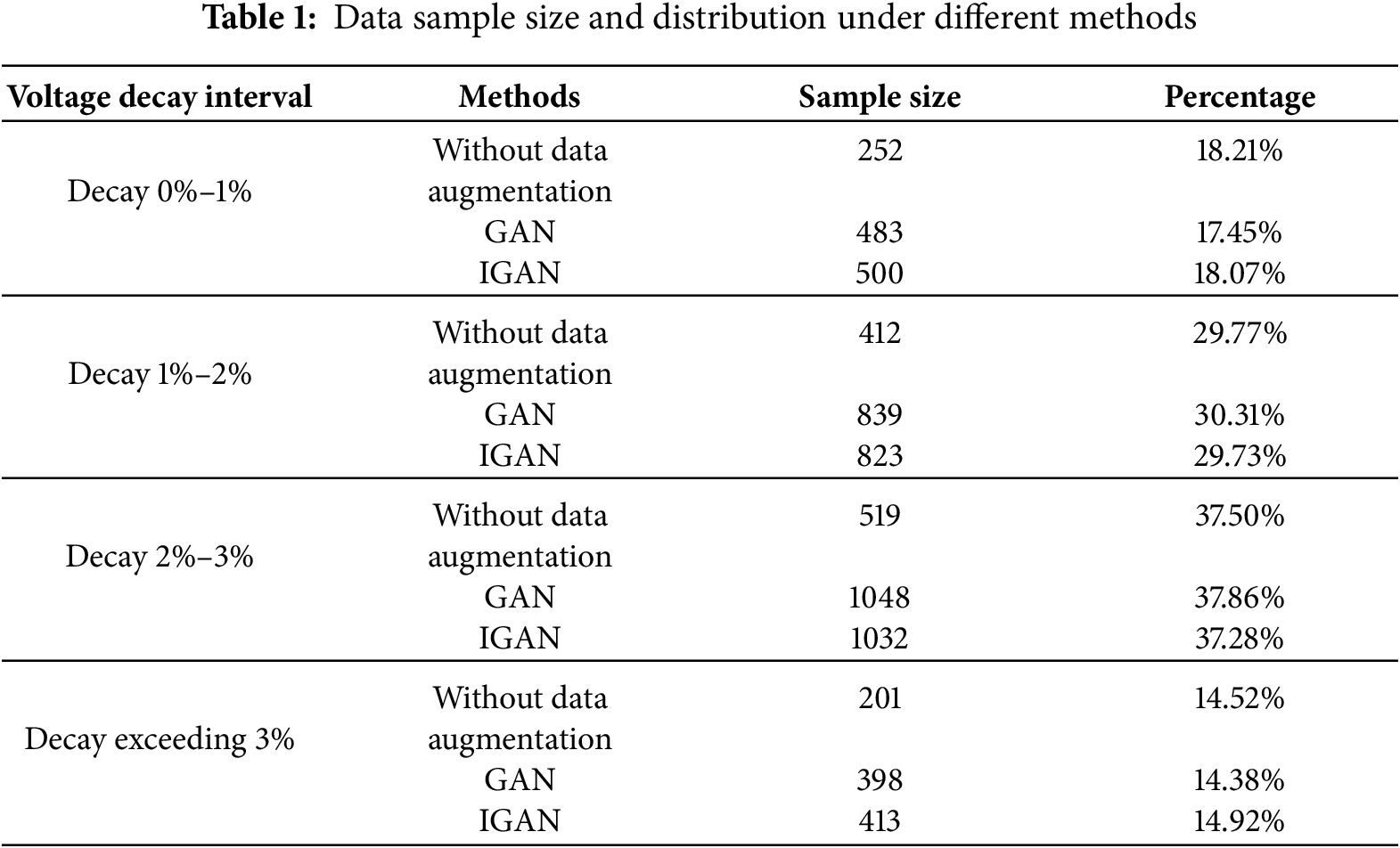
As can be seen from the table, in the original data, the distribution proportions in the 1%–2% decay interval and 2%–3% decay interval are relatively large, while the proportion of data with stack voltage decay greater than 3% is small, which is not conducive to the prediction of stack performance degradation. Through data augmentation methods such as GAN and IGAN, the number of stack prediction samples can be effectively increased, thereby improving the prediction accuracy. The data imbalance coefficients of the original data, the data augmented by GAN, and the data augmented by IGAN are 0.6128, 0.6202, and 0.5998, respectively.

The above conclusions indicate that data augmentation can effectively increase the number of samples. Furthermore, the sample features generated by the IGAN data augmentation method proposed in this paper are more consistent with the distribution of the original samples, and the degree of stack voltage imbalance in the generated samples has been improved.

4.3 PEMFC Performance Degradation Prediction

To check the enhancement brought by the proposed IGAN method to the prediction ability for PEMFC performance degradation, the real dataset is split into training data (60%) and prediction validation data (remaining 40%), and the real data is augmented with IGAN. For comparison, two more data groups are established: one augmented by GAN and the other using original real data. These three data groups are respectively used for prediction via the CNN-BiLSTM model, and the prediction outcomes are presented in Fig. 8.

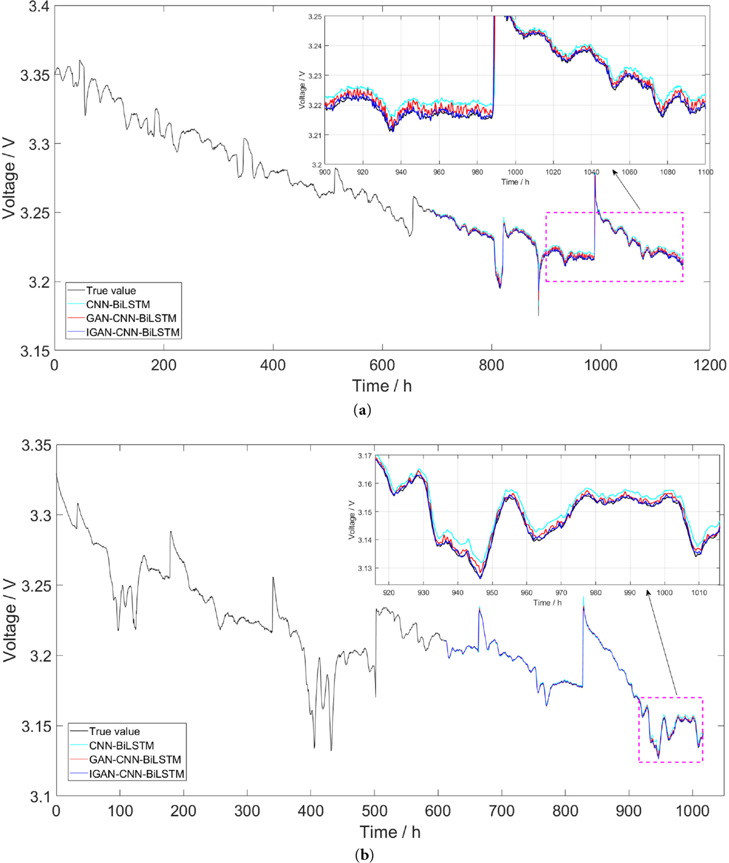
Figure 8: Prediction results by CNN-BiLSTM with different datasets. (a) FC1; (b) FC2

It can be seen from the Fig. 8 that in both FC1 and FC2 datasets, the CNN-BiLSTM method can well track the trend of PEMFC voltage changes, yet the error between predicted values and true values is notably larger than that of methods with data augmentation. In contrast, predicted values of the IGAN-CNN-BiLSTM method proposed in this paper basically overlap with the actual curve. To more intuitively show deviations between predicted values and true values of the three methods, residual plots and residual distribution plots of these three methods are presented in Figs. 9 and 10.

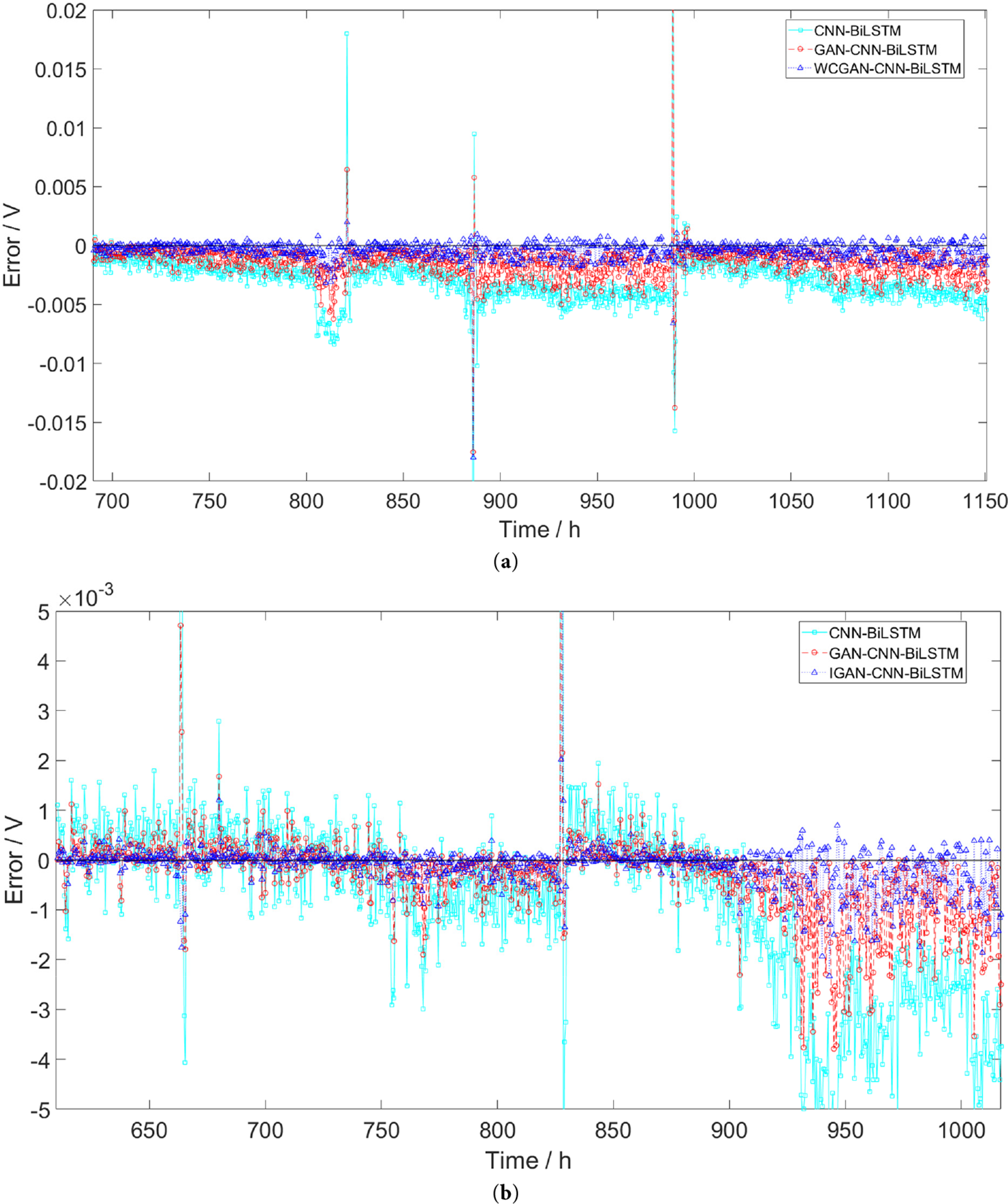
Figure 9: Residual of prediction results. (a) FC1; (b) FC2

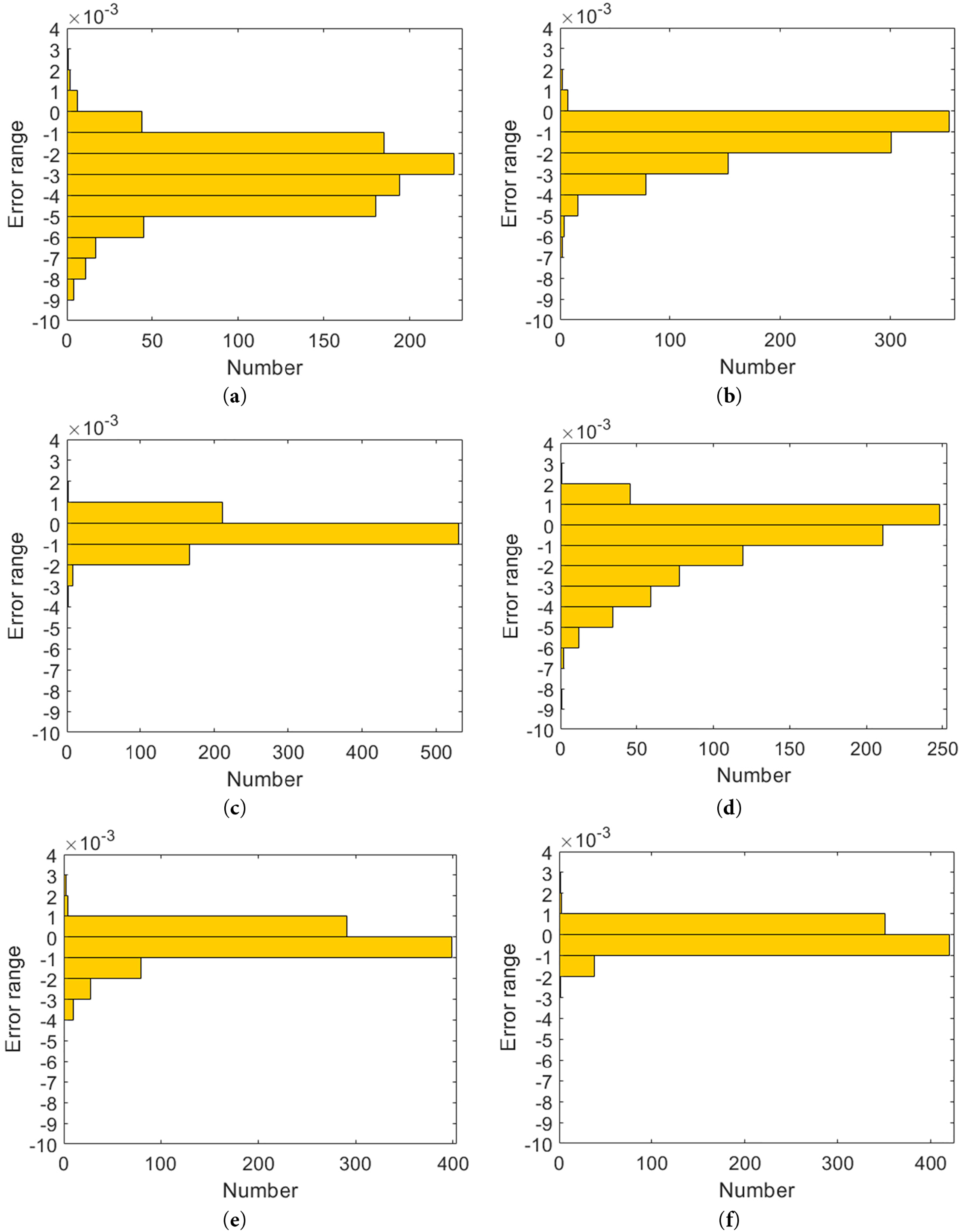
Figure 10: Residual distribution of prediction results. (a) FC1 by CNN-BiLSTM; (b) FC1 by GAN-CNN-BiLSTM; (c) FC1 by IGAN-CNN-BiLSTM; (d) FC2 by CNN-BiLSTM; (e) FC2 by GAN-CNN-BiLSTM; (f) FC2 by IGAN-CNN-BiLSTM

From residual plots and residual distribution plots, models based on data augmentation have smaller prediction errors, and their distributions are more concentrated and stable. In particular, the prediction error of this paper’s proposed IGAN-CNN-BiLSTM model is extremely small. This indicates that data augmentation is vital for enhancing the model’s prediction capability, and this paper’s proposed IGAN’s effect is superior to that of the original GAN.

Since this paper integrates the iGAN data augmentation and the CNN-BiLSTM prediction model, which consists of multiple components, we conduct ablation experiments to verify the role of each module in prediction. We use RMSE, Mean Absolute Percentage Error (MAPE), and Coefficient of Determination (R2) as performance metrics to evaluate the role of each module in prediction on the FC1 dataset. Meanwhile, training time and prediction time are used to measure the computational efficiency of each method. All time measurements are performed on the same computer platform, with the main configurations as follows: Matlab 2024a, Intel i9-13900H, RTX-4070 Ti. The results of the ablation experiments are listed in Table 2.

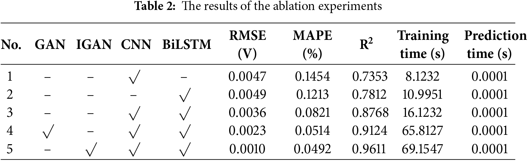
It can be seen form the results, CNN and BiLSTM perform less favorably than CNN-BiLSTM in terms of prediction model performance. After applying GAN for data augmentation, both RMSE and MAPE of the prediction results decrease, indicating a reduction in the error between the predicted values and the true values. The increase in R2 demonstrates that the prediction model achieves a better fitting effect on the data and exhibits higher accuracy in predicting fluctuating data. Following the improvement of GAN, all performance metrics are further enhanced, which verifies the effectiveness of all key components in the method proposed in this paper.

From the perspective of computational time, the proposed method in this paper exhibits a longer training time due to the incorporation of GAN; however, this increase is fully acceptable for long-term prediction tasks in PEMFC forecasting. Meanwhile, once the prediction model is trained, its inference time (for the prediction phase) is essentially consistent with that of other methods. Therefore, the model can be trained in an offline manner, and the offline-trained model can be deployed for online prediction.

4.4 PEMFC Performance Degradation Prediction by Different Prediction Methods

To verify how the proposed prediction approach performs under varying training set proportions, the share of training data for the prediction model is set to 40%, 50%, and 60%, respectively. The proposed approach is contrasted with other typical prediction techniques like CNN, BiLSTM, CNN-BiLSTM, and GAN-CNN-BiLSTM. Root mean square error (RMSE) is used to assess each model’s prediction performance, and each model’s prediction results are presented in Fig. 11.

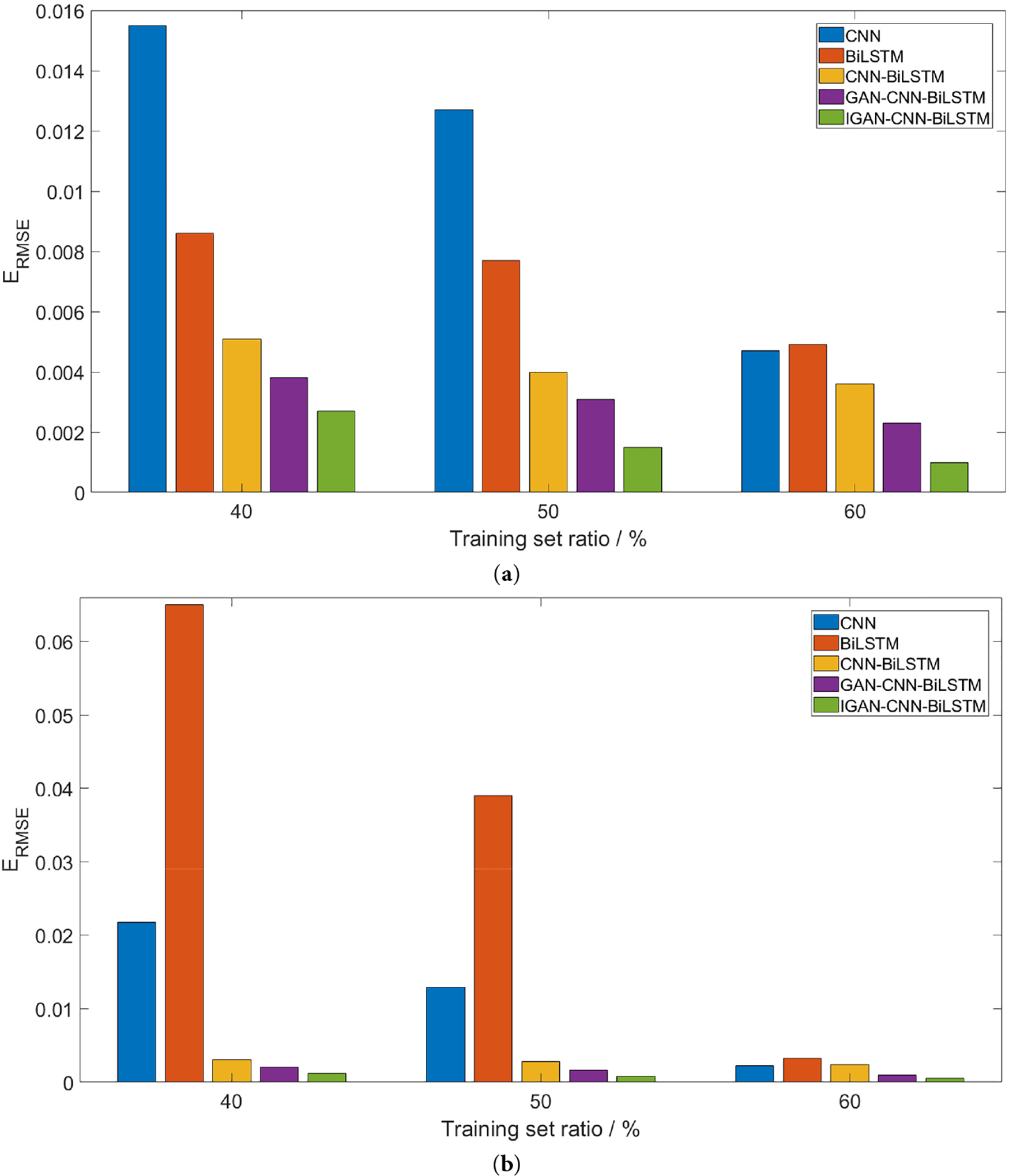
Figure 11: Prediction results by different methods with different training set ratio. (a) FC1; (b) FC2

Fig. 11 shows that each model’s prediction accuracy varies with different training set proportions of the dataset. When training data is limited, CNN and BiLSTM models’ prediction accuracy is significantly inferior to other methods. The CNN-BiLSTM model’s prediction performance has improved, indicating it can effectively extract features from historical PEMFC data and yield favorable prediction results. Results also show that data augmentation-based methods, especially this paper’s proposed method, have further enhanced prediction accuracy. This suggests that data augmentation methods can further enrich the feature information of PEMFC data, enabling accurate prediction of voltage variation trends.

5  Conclusions

To address the issue of insufficient and imbalanced data affecting the prediction accuracy of models in PEMFC performance degradation prediction, this paper proposes an improved GAN (IGAN) data augmentation method to augment the sample data, and adopts the CNN-BiLSTM prediction model to predict PEMFC performance degradation. The proposed method is validated using data under two operating conditions: stationary and quasi-dynamic. The conclusions are as follows:

(1)   Experiments show that the distribution of synthetic samples augmented by the proposed IGAN is similar to that of real samples in terms of data features. Compared with the over-concentration issue of samples generated by GAN, IGAN addresses inherent drawbacks such as gradient vanishing and can generate more abundant feature information.

(2)   The prediction models based on data augmentation exhibit significantly higher prediction accuracy than those that only use real samples. Data augmentation can notably enhance the performance of prediction models.

(3)   Comparative experiments indicate that the improvement in prediction accuracy of the proposed method mainly benefits from data augmentation and the CNN-BiLSTM prediction model. Furthermore, future studies could conduct further investigations into the network structure. Meanwhile, the present study has not addressed the issue of parameter selection in the model, which also merits attention in future research.

Acknowledgement: Not applicable.

Funding Statement: This work was supported by the Jiangsu Engineering Research Center of the Key Technology for Intelligent Manufacturing Equipment and the Suqian Key Laboratory of Intelligent Manufacturing (Grant No. M202108).

Author Contributions: The authors confirm contribution to the paper as follows: Conceptualization, Xiaolu Wang and Xin Xia; methodology, Xiaolu Wang; software, Haoyu Sun and Aiguo Wang; validation, Haoyu Sun and Aiguo Wang; formal analysis, Xiaolu Wang; data curation, Xiaolu Wang; writing—original draft preparation, Xiaolu Wang. All authors reviewed the results and approved the final version of the manuscript.

Availability of Data and Materials: The data that support the findings of this study are available from the Corresponding Author, [Xin Xia], upon reasonable request.

Ethics Approval: Not applicable.

Conflicts of Interest: The authors declare no conflicts of interest to report regarding the present study.

References

1. Mensharapov RM, Ivanova NA, Spasov DD, Bakirov AV, Fateev VN. PEMFC performance at nonstandard operating conditions: a review. Int J Hydrog Energy. 2024;96(79):664–79. doi:10.1016/j.ijhydene.2024.11.395. [Google Scholar] [CrossRef]

2. Cai F, Cai S, Tu Z. Proton exchange membrane fuel cell (PEMFC) operation in high current density (HCDproblem, progress and perspective. Energy Convers Manag. 2024;307:118348. doi:10.1016/j.enconman.2024.118348. [Google Scholar] [CrossRef]

3. Chen JH, He P, Cai SJ, He ZH, Zhu HN, Yu ZY, et al. Modeling and temperature control of a water-cooled PEMFC system using intelligent algorithms. Appl Energy. 2024;372(1):123790. doi:10.1016/j.apenergy.2024.123790. [Google Scholar] [CrossRef]

4. Jia C, He H, Zhou J, Li K, Li J, Wei Z. A performance degradation prediction model for PEMFC based on bi-directional long short-term memory and multi-head self-attention mechanism. Int J Hydrogen Energy. 2024;60:133–46. doi:10.1016/j.ijhydene.2024.02.181. [Google Scholar] [CrossRef]

5. Petrone R, Zheng Z, Hissel D, Péra MC, Pianese C, Sorrentino M, et al. A review on model-based diagnosis methodologies for PEMFCs. Int J Hydrogen Energy. 2013;38(17):7077–91. doi:10.1016/j.ijhydene.2013.03.106. [Google Scholar] [CrossRef]

6. Deng Z, Chen M, Wang H, Chen Q. Performance-oriented model learning and model predictive control for PEMFC air supply system. Int J Hydrogen Energy. 2024;64(17):339–48. doi:10.1016/j.ijhydene.2024.01.351. [Google Scholar] [CrossRef]

7. Wang B, Xie B, Xuan J, Jiao K. AI-based optimization of PEM fuel cell catalyst layers for maximum power density via data-driven surrogate modeling. Energy Convers Manag. 2020;205(7):112460. doi:10.1016/j.enconman.2019.112460. [Google Scholar] [CrossRef]

8. He K, Zhang C, He Q, Wu Q, Jackson L, Mao L. Effectiveness of PEMFC historical state and operating mode in PEMFC prognosis. Int J Hydrogen Energy. 2020;45(56):32355–66. doi:10.1016/j.ijhydene.2020.08.149. [Google Scholar] [CrossRef]

9. Deng S, Zhang J, Zhang C, Luo M, Ni M, Li Y, et al. Prediction and optimization of gas distribution quality for high-temperature PEMFC based on data-driven surrogate model. Appl Energy. 2022;327:120000. doi:10.1016/j.apenergy.2022.120000. [Google Scholar] [CrossRef]

10. Shin S, Kim J, Lee S, Shin TH, Ryu GA. Multimodal data-driven prediction of PEMFC performance and process conditions using deep learning. IEEE Access. 2024;12:168030–42. doi:10.1109/ACCESS.2024.3472849. [Google Scholar] [CrossRef]

11. Elkholy M, Boureima A, Kim J, Aziz M. Data-driven modeling and prediction of PEM fuel cell voltage response to load transients for energy applications. Energy. 2025;335:138047. doi:10.1016/j.energy.2025.138047. [Google Scholar] [CrossRef]

12. Jin J, Chen Y, Xie C, Wu F. Degradation prediction of PEMFC based on data-driven method with adaptive fuzzy sampling. IEEE Trans Transp Electrif. 2024;10(2):3363–72. doi:10.1109/TTE.2023.3296719. [Google Scholar] [CrossRef]

13. Yan F, Lu H, Yao J, Pei X, Feng S, Zhao C. Optimizing interleaved distributed streamline obstacle flow channels through genetic algorithm coupled with backpropagation neural network regression predictive surrogate model. Fuel. 2024;372(19):132174. doi:10.1016/j.fuel.2024.132174. [Google Scholar] [CrossRef]

14. Quan R, Liang W, Wang J, Li X, Chang Y. An enhanced fault diagnosis method for fuel cell system using a kernel extreme learning machine optimized with improved sparrow search algorithm. Int J Hydrogen Energy. 2024;50(2):1184–96. doi:10.1016/j.ijhydene.2023.10.019. [Google Scholar] [CrossRef]

15. Liu Q, Zang W, Zhang W, Zhang Y, Tong Y, Feng Y. Steady-state model enabled dynamic PEMFC performance degradation prediction via recurrent neural network. Energies. 2025;18(10):2665. doi:10.3390/en18102665. [Google Scholar] [CrossRef]

16. Li W, Wang X, Wang L, Jia L, Song R, Fu Z, et al. An LSTM and ANN fusion dynamic model of a proton exchange membrane fuel cell. IEEE Trans Ind Inform. 2023;19(4):5743–51. doi:10.1109/TII.2022.3196621. [Google Scholar] [CrossRef]

17. Tao Z, Zhang C, Xiong J, Hu H, Ji J, Peng T, et al. Evolutionary gate recurrent unit coupling convolutional neural network and improved manta ray foraging optimization algorithm for performance degradation prediction of PEMFC. Appl Energy. 2023;336:120821. doi:10.1016/j.apenergy.2023.120821. [Google Scholar] [CrossRef]

18. Chen D, Wu W, Chang K, Li Y, Pei P, Xu X. Performance degradation prediction method of PEM fuel cells using bidirectional long short-term memory neural network based on Bayesian optimization. Energy. 2023;285(3):129469. doi:10.1016/j.energy.2023.129469. [Google Scholar] [CrossRef]

19. Sun B, Liu X, Wang J, Wei X, Yuan H, Dai H. Short-term performance degradation prediction of a commercial vehicle fuel cell system based on CNN and LSTM hybrid neural network. Int J Hydrogen Energy. 2023;48(23):8613–28. doi:10.1016/j.ijhydene.2022.12.005. [Google Scholar] [CrossRef]

20. Quan R, Zhang J, Li X, Guo H, Chang Y, Wan H. A hybrid CNN-BiLSTM–AT model optimized with enhanced whale optimization algorithm for remaining useful life forecasting of fuel cell. AIP Adv. 2024;14(2):025251. doi:10.1063/5.0191483. [Google Scholar] [CrossRef]

21. Peng Y, Chen T, Xiao F, Zhang S. Remaining useful lifetime prediction methods of proton exchange membrane fuel cell based on convolutional neural network-long short-term memory and convolutional neural network-bidirectional long short-term memory. Fuel Cells. 2023;23(1):75–87. doi:10.1002/fuce.202200106. [Google Scholar] [CrossRef]

22. Quan R, Cheng G, Guan X, Zhang G, Quan J. A HO-BiGRU-Transformer based PEMFC degradation prediction method under different current conditions. Renew Energy. 2026;256(2):124132. doi:10.1016/j.renene.2025.124132. [Google Scholar] [CrossRef]

23. Anu Shalini T, Sri Revathi B. Power generation forecasting using deep learning CNN-based BILSTM technique for renewable energy systems. J Intell Fuzzy Syst. 2022;43(6):8247–62. doi:10.3233/jifs-220307. [Google Scholar] [CrossRef]

24. Andújar JM, Segura F. PEFC simulator and real time monitoring system. Fuel Cells. 2015;15(6):813–25. doi:10.1002/fuce.201500128. [Google Scholar] [CrossRef]

25. Liu Z, Sun H, Xu L, Mao L, Hu Z, Li J. Toward low-data and real-time PEMFC diagnostic: multi-sine stimulation and hybrid ECM-informed neural network. Appl Energy. 2025;391(4):125959. doi:10.1016/j.apenergy.2025.125959. [Google Scholar] [CrossRef]

26. Branikas E, Murray P, West G. A novel data augmentation method for improved visual crack detection using generative adversarial networks. IEEE Access. 2023;11:22051–9. doi:10.1109/ACCESS.2023.3251988. [Google Scholar] [CrossRef]

27. Ge Q, Li J, Lacasse S, Sun H, Liu Z. Data-augmented landslide displacement prediction using generative adversarial network. J Rock Mech Geotech Eng. 2024;16(10):4017–33. doi:10.1016/j.jrmge.2024.01.003. [Google Scholar] [CrossRef]

28. Gao X, Deng F, Yue X. Data augmentation in fault diagnosis based on the Wasserstein generative adversarial network with gradient penalty. Neurocomputing. 2020;396(99):487–94. doi:10.1016/j.neucom.2018.10.109. [Google Scholar] [CrossRef]

29. Jin Q, Lin R, Yang F. E-WACGAN: enhanced generative model of signaling data based on WGAN-GP and ACGAN. IEEE Syst J. 2020;14(3):3289–300. doi:10.1109/JSYST.2019.2935457. [Google Scholar] [CrossRef]

30. Goodfellow I, Pouget-Abadie J, Mirza M, Xu B, Warde-Farley D, Ozair S, et al. Generative adversarial networks. Commun ACM. 2020;63(11):139–44. doi:10.1145/3422622. [Google Scholar] [CrossRef]

31. Huo W, Li W, Zhang Z, Sun C, Zhou F, Gong G. Performance prediction of proton-exchange membrane fuel cell based on convolutional neural network and random forest feature selection. Energy Convers Manag. 2021;243(2):114367. doi:10.1016/j.enconman.2021.114367. [Google Scholar] [CrossRef]

32. Lu W, Li J, Wang J, Qin L. A CNN-BiLSTM-AM method for stock price prediction. Neural Comput Appl. 2021;33(10):4741–53. doi:10.1007/s00521-020-05532-z. [Google Scholar] [CrossRef]

33. Hua Z, Zheng Z, Péra MC, Gao F. Remaining useful life prediction of PEMFC systems based on the multi-input echo state network. Appl Energy. 2020;265:114791. doi:10.1016/j.apenergy.2020.114791. [Google Scholar] [CrossRef]