
 Submit a Paper
 Propose a Special lssue
 Open Access
ARTICLE

Modeling Techno-Economic Boundaries for Undeveloped Reservoirs: Integrated Simulation-Regression Approach with Xinjiang Case Study
1 Petroleum Exploration and Development Institute, Xinjiang Oilfield Company, Karamay, 834000, China
2 School of Economics and Management, Southwest Petroleum University, Chengdu, 610500, China
* Corresponding Author: Xin-Jian Zhao. Email:
Energy Engineering 2026, 123(3), 24 https://doi.org/10.32604/ee.2025.071943
Received 16 August 2025; Accepted 24 October 2025; Issue published 27 February 2026
 View Full Text
 Download PDF
Abstract
Traditional oilfields face increasing extraction challenges, primarily due to reservoir quality degradation and production decline, which are further exacerbated by volatile international crude oil prices—illustrated by Brent Crude’s trajectory from pandemic-induced negative pricing to geopolitically driven surges exceeding USD 100 per barrel. This study addresses these complexities through an integrated methodological framework applied to medium-permeability sandstone reservoirs in the Xinjiang oilfield by combining advanced numerical simulations with multivariate regression analysis. The methodology employs Latin Hypercube Sampling (LHS) to stratify geological parameter distributions and constructs heterogeneous reservoir models using Petrel software, rigorously validated through historical production data matching. Production forecasting integrates numerical simulation and Decline Curve Analysis (DCA), while investment estimation utilizes Ordinary Least Squares (OLS) regression to correlate engineering parameters with drilling and completion costs. Economic evaluation incorporates Discounted Cash Flow (DCF) modeling and breakeven analysis, establishing techno-economic boundaries via oil price sensitivity analysis ranging from USD 40 to 90 per barrel. Visualization tools, including 3D heatmaps, delineate nonlinear interactions among engineering, geological, and investment datasets under economic constraints. Key findings demonstrate that for the target reservoirs, as oil prices increase from USD 40 to USD 90 per barrel, the minimum economic thickness threshold decreases from approximately 5.7 m to about 2.5 m, with model prediction errors consistently below 25% across validation datasets. This framework provides scientifically grounded decision support for optimizing capital allocation and offers actionable insights to enhance undeveloped hydrocarbon development planning amid market uncertainty. Ultimately, it supports national energy security through technically robust and economically viable resource exploitation strategies.Keywords
According to data from the International Energy Agency (2023) [1], the petrochemical sector remains the primary driver of global oil demand growth. Liquefied petroleum gas (LPG), ethane, and naphtha account for over 50% of the incremental growth from 2022 to 2028 and nearly 90% of the growth relative to pre-pandemic levels. Additionally, international oil prices have experienced significant volatility in recent years. In 2020, West Texas Intermediate (WTI) crude futures prices briefly turned negative due to the pandemic, while geopolitical conflicts pushed prices above USD 100 per barrel in 2022. In the first quarter of 2024, Brent crude futures surged past USD 90 per barrel amid escalating conflicts, with the annual average Brent price stabilizing at USD 79.86 per barrel. To safeguard national and regional energy security and enhance the economic efficiency of oilfield companies amid rapid oil price fluctuations, Nandi et al. (2024) [2] and Popescu and Gheorghiu (2021) [3] emphasize the need to implement measures that mitigate external shocks. This necessitates the development of a rapid, accurate, and intuitive techno-economic evaluation methodology to support agile decision-making.
This study begins with production forecasting for tight sandstone oil reservoirs, followed by the development of drilling and production investment models. Finally, technical-economic boundary charts were created by integrating factors such as well costs, special oil income levies, and international oil prices, accompanied by an operational manual. The charts demonstrate that, within a USD 40–90 price range, the minimum required Estimated Ultimate Recovery (EUR) for sandstone tight oil reservoirs decreases as oil prices increase. These boundary charts offer a framework for optimizing investment project designs, facilitating rapid decision-making to ensure cost-effective, large-scale oilfield development.
Reservoir production forecasting employs several approaches. For example, teams led by Wang et al. [4], Liu et al. [5], and Dou et al. [6] utilized waterflood curve methods, which involve semi-logarithmic plots of cumulative water production vs. cumulative oil production based on comprehensive production data. This method fits coefficients for waterflood curve models and is suitable for mid-stage reservoir development and forecasting overall production trends. Kaiser [7], Makinde and Lee [8] applied empirical decline curve analysis, fitting historical production data to various decline models to predict future output, making it appropriate for mid-to-late reservoir development with extended decline phases. Although these methods are simple and efficient, they are time-bound and require additional petrophysical parameters for accuracy when employing numerical simulation. Feng et al. (2022) [9] developed mathematical-physical reservoir models to simulate subsurface fluid flow, enabling production forecasting independent of development stages.
For investment prediction methodologies, Redutskiy [10] and Wang et al. [11] applied cost structure analysis to evaluate oilfield investments, while Yang et al. [12] utilized machine learning to forecast dynamic shale gas drilling investments. However, cost structure analysis overlooks inter-cost correlations, and neural network models function as “black boxes,” limiting interpretability. Zhu [13] employed regression analysis, establishing explicit mathematical relationships between investments and influencing factors using historical data. This approach addresses issues related to variable correlation and interpretability. Consequently, regression analysis incorporating engineering parameters was prioritized in this study for single-well investment prediction.
Jang et al. [14] proposed using techno-economic boundary charts to identify critical parameter thresholds, combined with NPV analysis, to assess project feasibility. In energy development projects and utilization processes, Abbas et al. [15] conducted techno-economic evaluations by comparing process and operational costs across different solutions. Similarly, Armoo et al. [16] enhanced these evaluations by incorporating financial indicators such as NPV, internal rate of return (IRR), and simple payback period. However, Li et al. [17] noted that standalone financial indicator analyses do not facilitate rapid decision-making with intuitive visualization, such as boundary charts, making chart-based approaches essential. This study integrates key parameters—including international oil prices, oil saturation, effective reservoir thickness, and production limits—to develop multi-scenario techno-economic boundary charts. These visual tools support rational resource allocation and investment decision-making in oilfields.
This paper is organized as follows: Section 2 provides a comprehensive literature review of existing research methodologies related to EUR prediction, investment forecasting, and techno-economic evaluation for oilfield development, highlighting advancements and limitations in the field. Section 3 outlines the integrated methodology, which combines numerical simulation and multiple regression analysis to establish techno-economic boundary models for undeveloped reservoirs. Specifically, production forecasting is conducted using numerical simulation, while investment costs are estimated through regression analysis of engineering parameters. These models are integrated with discounted cash flow and break-even analyses to facilitate rapid techno-economic evaluation of untapped resources. Section 4 presents the results and discussion, validating the accuracy of production forecasts, the reliability of investment predictions, and the economic viability across different reservoir types under fluctuating oil prices. Techno-economic limit charts illustrate the interdependencies among EUR, investment thresholds, and oil prices, while highlighting disparities between reservoir categories and development strategies. Subsequently, a single-factor sensitivity analysis is performed. Section 5 concludes the paper by synthesizing key findings and discussing their implications for optimizing field development decisions.
The development of prediction methods for the EUR of oil is relatively advanced. Early research primarily focused on production decline curve analysis, specifically empirical decline methods. The Arps decline model is one of the principal empirical decline methods. The classical production forecasting model proposed by Arps [18] is widely used to analyze production decline patterns in conventional oil and gas reservoirs during their middle and late development stages. However, its assumptions are stringent, making it suitable only for wells with stable production regimes and boundary-dominated flow, and limiting its applicability to unconventional oil and gas predictions. Sharma and Lee [19] innovatively combined diagnostic plots with the Arps and Duong models, enhancing prediction capabilities for ultra-low permeability reservoirs through data smoothing techniques. This approach enabled precise differentiation between transient flow and boundary-dominated flow stages, significantly improving prediction accuracy.
Simulation prediction methods include analytical and numerical simulations. Although numerical simulation involves a longer modeling cycle and greater computational complexity, it offers the advantage of higher prediction accuracy. With increasing computational power, numerical simulation is being applied more extensively in reservoir EUR prediction, with continuously improving accuracy. Wu et al. [20] conducted experiments on the effect of displacement pressure gradient on oil–water relative permeability and established a correction model based on the Willhite model. Their results indicate that relative permeability varies with displacement pressure gradient, influencing production performance and residual oil distribution. Integrating this model into the MRST enabled dynamic representation of relative permeability in reservoir simulation. Sikanyika et al. [21] employed a black-oil model in Schlumberger’s ECLIPSE simulator to simulate a layered heterogeneous reservoir under water injection and compared the performance of horizontal and vertical wells. Through 25 simulation runs, horizontal wells demonstrated significantly higher productivity than vertical wells, suggesting the need to optimize water injection rates and the number of injection wells. Further analysis indicated that reservoir thickness positively influenced the productivity of both well types. To enhance oil recovery, increasing the horizontal well length was recommended to expand reservoir contact.
Regarding oilfield investment prediction, factors such as material prices, oil prices, and operational costs all influence oilfield profitability. In the field of oilfield techno-economic evaluation, numerous evaluation systems and methods have been developed in academia. Shi et al. [22], using the Microsoft Azure machine learning platform, employed algorithms such as neural networks, boosted decision trees, and decision forests to perform dynamic modeling of oilfield development costs. Their study demonstrated that by applying the Permutation Feature Importance (PFI) model, key influencing factors can be identified, providing effective scientific decision support for oil companies and enabling more accurate and efficient estimation and prediction of oilfield assets. Chen et al. [23] conducted a systematic review of the applications of BP neural networks, radial basis function neural networks, generalized regression neural networks, and wavelet neural networks in predicting key development indicators such as oil production volume, liquid production volume, water content, as well as costs and profits. Through case studies, they demonstrated that the prediction accuracy and stability of the WOA-BPNN model were significantly superior to those of traditional methods and the benchmark ANN model.
In summary, existing research has developed a relatively comprehensive system of EUR prediction methods. Compared to decline curve analysis and other approaches, numerical simulation provides higher prediction accuracy and broader applicability, but it involves a longer modeling cycle and greater model complexity. Regarding reservoir investment prediction, due to the volatility of actual investment amounts, most studies employ multiple regression models to provide rough estimates of reservoir investment levels. In reservoir economic evaluation, academia currently offers a diverse range of evaluation systems tailored to reservoirs with varying characteristics and objectives, primarily focusing on economic factors from the perspective of economic limits.
3 Equations and Mathematical Expressions
3.1 Production Prediction Model
The production prediction model is developed by employing Latin Hypercube Sampling (LHS) to gather geological data, performing history matching for model calibration and validation, and subsequently constructing a numerical simulation model using parameters obtained from the history-matched model to forecast reservoir production.
The LHS method was employed to generate multiple sets of reservoir property data, including porosity, permeability, oil saturation, and effective thickness, based on their respective distribution ranges. Using parameters derived from historical fitting models, this approach predicts the production performance of inverted seven-spot waterflood well patterns and single wells under various combinations of reservoir properties.
The LHS workflow consists of the following steps:
Step 1: Define the number of variable dimensions, sample size, and distribution ranges for each variable.
Step 2: Partition the variable space into non-overlapping subintervals, assigning equal probability to each subinterval.
Step 3: Randomly select one sampling point within each sub-interval for every variable, ensuring that each sub-interval contains exactly one sample.
Step 4: Randomize the order of sampling points to ensure uniform coverage across the entire parameter space.
3.1.2 Numerical Simulation Model
A heterogeneous numerical simulation model was developed using Petrel software, based on mathematical and physical principles. Grid spacing was defined, and parameters such as oil-water relative permeability, capillary pressure, permeability, and fluid properties were calibrated. Daily oil and water production rates for individual wells were simulated, with iterative adjustments to model parameters made to match actual production data and validate the historical simulation.
3.2 Investment Prediction Model
The correlation between engineering parameters and investment components was analyzed, with drilling investment and production investment designated as dependent variables. Based on the correlation analysis results and practical considerations, engineering parameters exhibiting strong correlations with each type of investment were selected as explanatory variables. Subsequently, multiple regression models for the target reservoir were constructed using these selected explanatory variables.
Ordinary least squares (OLS) regression was used to fit the model, assuming linear relationships between variables. The dataset was split so that 80% served as the training set for model fitting, while the remaining 20% was reserved as the test set for model validation and optimization.
For variables demonstrating statistically significant linear relationships, linear regression models were applied. For variables exhibiting significant monotonic but nonlinear relationships, appropriate nonlinear functional forms were identified through a literature review and subsequent evaluation following correlation analysis.
3.2.1 Correlation Analysis Tool
A statistical technique for measuring the connections between two or more variables is correlation analysis. Hypothesis testing and correlation coefficients are important ideas. Table 1 lists the popular correlation analysis techniques along with their suitability.
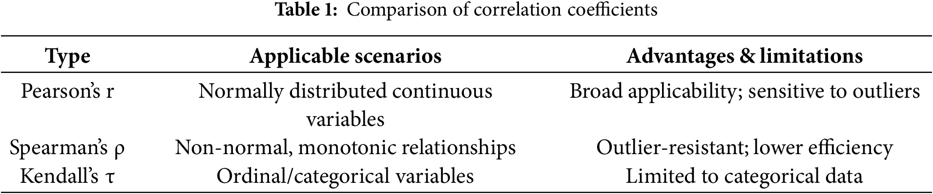
The Pearson’s correlation coefficient is used in this study to assess the connections between investments and engineering factors. The definition of the Pearson coefficient
where
Regression parameters are estimated using the least squares method, which minimizes the sum of squared residuals between predicted and observed values. Regarding a linear model:
the objective function is:
where
where
Finding parameters that are highly correlated with different investment categories using correlation analysis makes it possible to build regression models that accurately forecast future investment levels.
The cost framework for economic evaluation aligns with oil and gas production processes and encompasses 11 primary operational cost categories. Each cost item is analyzed based on its directly associated operational metrics and valuation methods, establishing a foundation for categorized cost estimation. In the Xinjiang Oilfield, costs are divided into operational costs, business taxes, and income taxes. Operational costs include direct operating expenses, administrative fees, financial costs, and depreciation, while business taxes consist of urban maintenance and construction tax, education surcharges, mining rights transfer fees, and special oil income levies. By analyzing these components, the unit fully allocated cost (FAC) is derived, integrating production and investment forecasts to predict future reservoir cost profiles. This forms the basis for the Xinjiang Oilfield’s categorized cost valuation model.
The unit FAC is defined as follows:
where
where
Total depreciation:
where
Abandonment cost:
where
Urban maintenance tax:
where
Mining rights fee:
where
Value-added tax (VAT):
where
Historical reservoir development cost data are analyzed to parameterize these models. Reservoir types, selected based on production and investment forecasts, are used to calibrate cost-related variables, ensuring alignment with specific operational and geological conditions. This systematic approach enables robust cost prediction and supports optimized decision-making for oilfield development.
3.3 Economic Evaluation Models
The DCF model consists of the NPV model and the IRR model. The NPV model is an investment valuation method based on the principle of NPV calculation, used to assess the value of an investment project or enterprise at the current point in time. NPV refers to the present value obtained by discounting future cash flows at a specific discount rate and then subtracting the initial investment cost. It reflects the absolute return on the project investment and serves as a key indicator for evaluating whether an investment project is worthwhile. Its fundamental calculation formula is:
where
The NPV model incorporates factors such as production volume, investment, and costs into the calculation of net present value. It is used to evaluate the economic feasibility and profitability of reservoir investments under varying production and investment levels throughout their lifecycle.
By calculating and analyzing cash flows, the model evaluates the value of oilfield development investments at the present time, expressed as the NPV. By varying the discount rate
where
IRR is a key metric that provides a comprehensive quantitative analysis of an investment’s rate of return by considering both the principal amount and the timing of cash flows. The IRR represents the discount rate at which the NPV of the investment equals zero, effectively serving as the “investment rate of return.” If the calculated IRR exceeds the prevailing market interest rate at the time the contract is executed, the investor can expect to earn a profit.
The IRR is determined by finding the discount rate that makes the Net Present Value (NPV) equal to zero. The process begins by identifying the project’s cash flows, including the initial investment outlay and the subsequent annual cash inflows and outflows. Next, a discount rate
The Break-Even Point (BEP) is a fundamental concept in economics, referring to the point at which a company’s total revenue equals its total costs under specific operating conditions. In this study, it is defined by the following formulas:
where
Based on the break-even principle, the lower economic limit thickness is calculated, leading to the development of the economic threshold model. By applying different oil prices (OP), the production volume and investment level at which revenue equals cost are determined. This process yields two models: the Limit Production–Limit Investment Model (with production as the dependent variable and investment as the independent variable) and the Limit Investment–Limit Production Model (with investment as the dependent variable and production as the independent variable). Using the previously established production and investment prediction models, the economic threshold model is further refined: the Limit Investment–Limit Production Model is decomposed into a Limit Investment–Rock Property Parameter Model, and the Limit Production–Limit Investment Model is decomposed into a Limit Production–Engineering Parameter Model.
4.1 Production Forecasting Model
4.1.1 Preliminary Data Organization
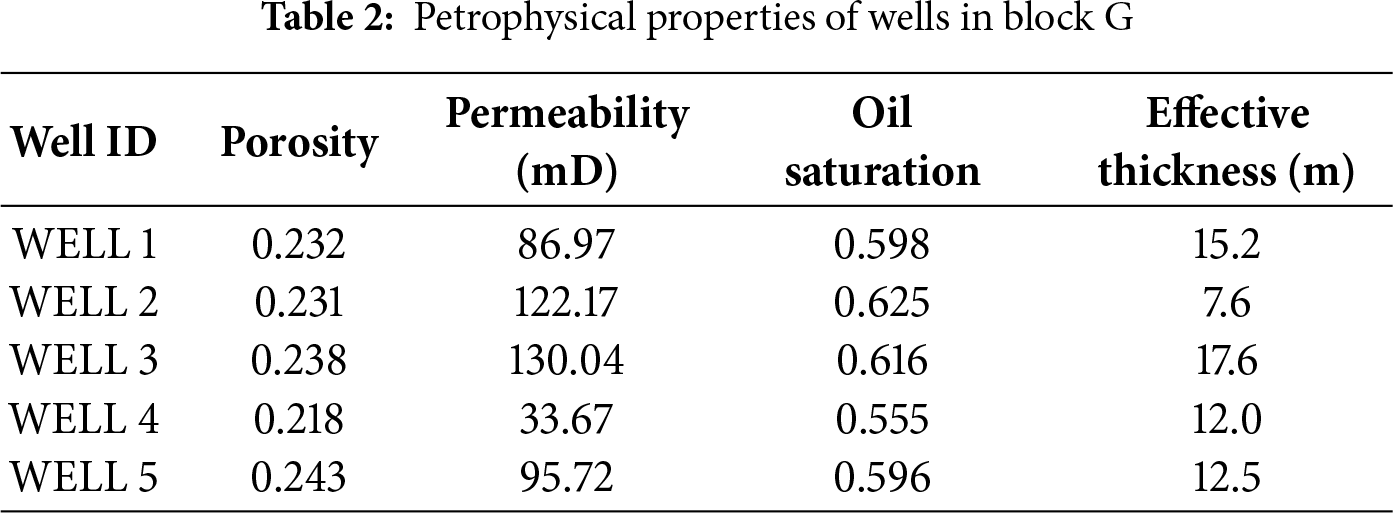
Typical well groups were selected for analysis using the LHS method. The target area, Block G, is a sandstone reservoir with moderate permeability, developed using an inverted seven-spot waterflood pattern. The petrophysical parameters of Block G are presented in Table 2. A heterogeneous numerical simulation model was constructed in Petrel based on the petrophysical parameters of the selected wells. The model grid resolution is 5 m × 5 m, with an average porosity of 23.26%, permeability of 93.36 mD, oil saturation of 59.87%, and an effective thickness of 13.65 m.
4.1.2 Numerical Simulation Model
A heterogeneous numerical simulation model was developed for the well group, which consists of six production wells and one central injection well, based on mathematical and physical principles. Parameters such as oil-water relative permeability, capillary pressure, permeability, and fluid properties were calibrated to simulate the daily oil and water production rates for each well. The historical matching period spanned from August 2019 to October 2024, with simulation results presented in Figs. 1–4. Fig. 1 shows the heterogeneous numerical simulation model, while Fig. 2 displays the oil-water relative permeability and capillary pressure curves. Fig. 3a,b presents the simulated liquid flow rates of selected wells within the group. Fig. 4a illustrates the simulated oil production efficiency, and Fig. 4b shows the simulated water cut. Analysis of the results demonstrates close agreement between simulated and actual values for liquid flow rates, oil production efficiency, and water cut, confirming the model’s reliability.
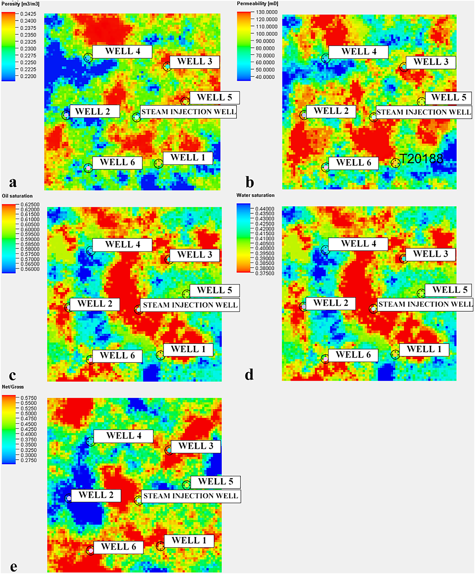
Figure 1: Heterogeneous numerical simulation model: (a) Porosity model; (b) Permeability model; (c) Oil saturation model; (d) Water saturation model; (e) NTG model
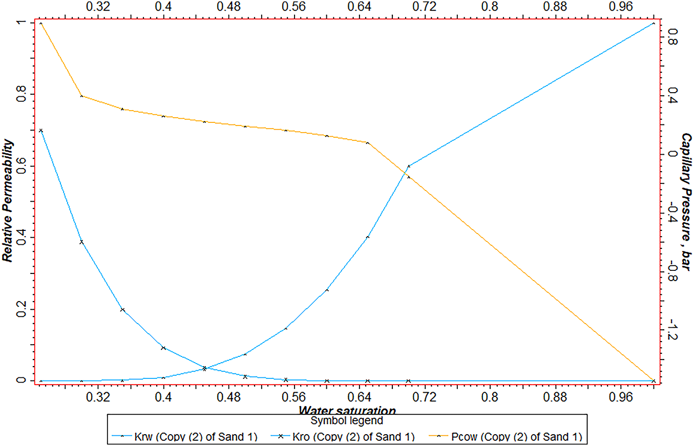
Figure 2: Oil-Water relative permeability and capillary pressure curves
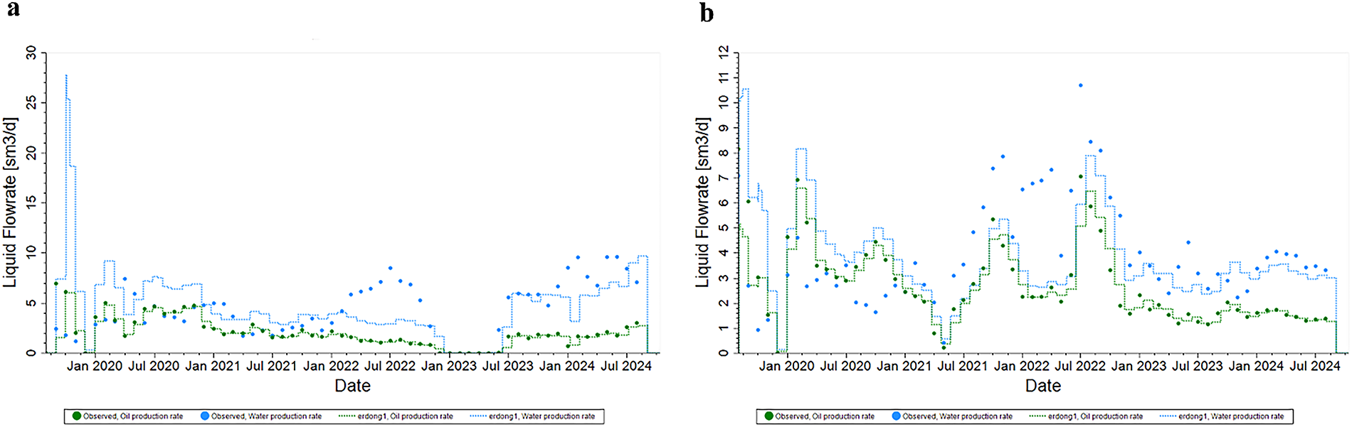
Figure 3: Simulated liquid flow rates of representative wells: (a) Well 1; (b) Well 3
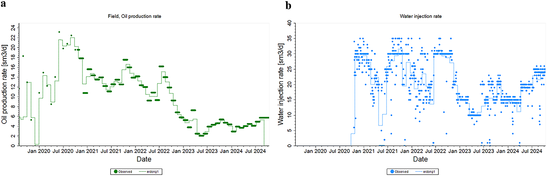
Figure 4: Simulated oil production efficiency and water cut: (a) oil production efficiency; (b) water cut
Based on the historically matched model, a 10-year production forecast was conducted under the current operational regime. The cumulative oil production of the well group and the average EUR per well were predicted. Fig. 5a,b illustrates the predicted daily oil production and daily water production of this well group, respectively. Fig. 6a,b shows the predicted daily oil production of several individual wells, respectively. The strong alignment between simulated and actual daily production data confirms the validity of the calibrated model parameters for production forecasting.
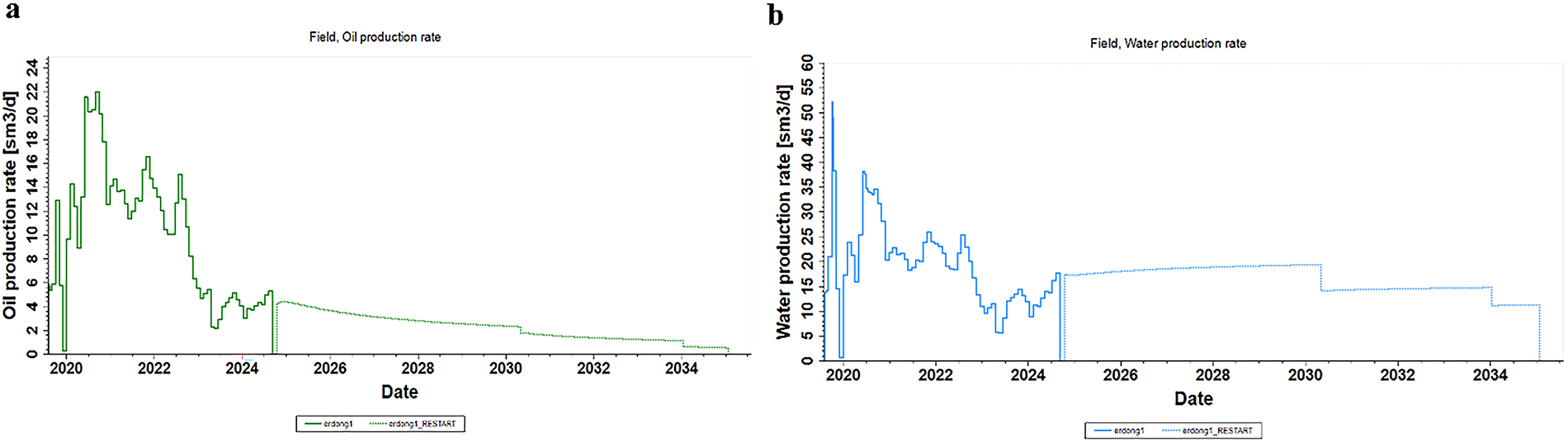
Figure 5: Daily oil and water production forecast for the well group: (a) oil production; (b) water production
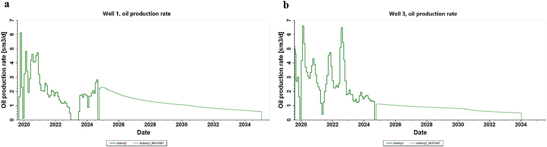
Figure 6: Daily oil production forecast for individual wells: (a) well 1; (b) well 3
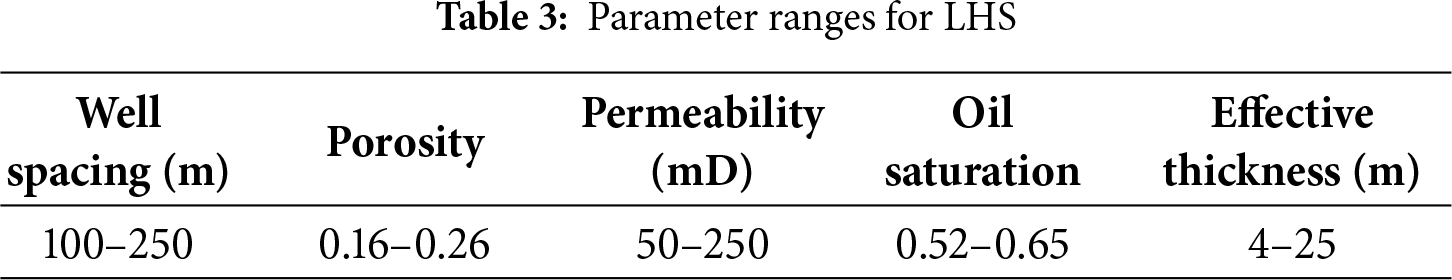
Using LHS method, 74 sets of parameters—including well spacing, porosity, permeability, oil saturation, and effective thickness—were generated within the property distribution ranges of the G Block reservoir (Table 3). These parameters, combined with historically matched model inputs, were used to predict production performance for inverted seven-spot waterflood patterns and individual wells under varying well spacing and petrophysical combinations.
The Pearson correlation coefficient matrix (Fig. 7) reveals that oil saturation, net pay thickness, and well spacing are the most influential factors affecting EUR in moderately permeable sandstone reservoirs. A strong positive linear correlation exists between EUR and first-year production, enabling the derivation of a highly accurate predictive formula (
where
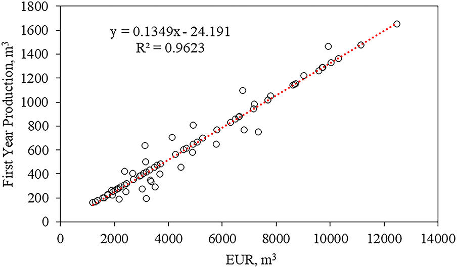
Figure 7: Relationship between first year production and EUR
4.1.4 Production Forecasting Results
Using the least squares method, a multivariate linear regression model was developed to predict EUR for inverted seven-spot waterflood patterns in moderately permeable sandstone reservoirs. The model, calibrated on historical and sampled production data, achieves an
where
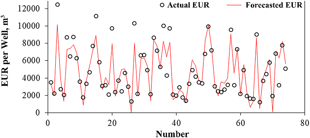
Figure 8: EUR prediction results on the dataset used for formula fitting
4.2 Investment Prediction Model
4.2.1 Engineering Parameter Data Overview
The overall parameter ranges are illustrated in Fig. 9a,b. The construction period primarily ranges from 5 to 20 days, while the vertical depth is concentrated between 1250 and 2250 m.
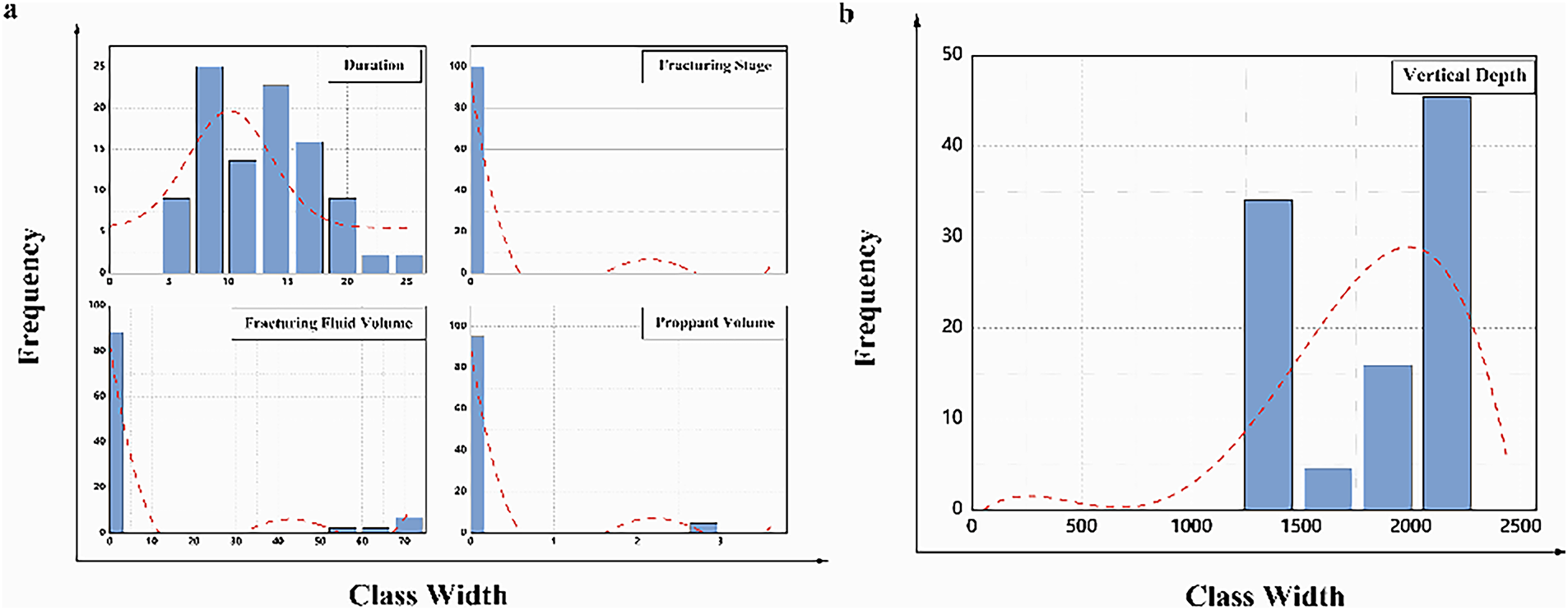
Figure 9: Frequency distribution histogram of (a) duration (day), fracturing stage, fracturing fluid volume (m3) and proppant volume (m3); (b) vertical depth (m)
4.2.2 Single-Parameter Preliminary Analysis
The preliminary regression results examining the relationship between investment and individual parameters are presented in Fig. 10. Specifically, Fig. 10a illustrates the relationship between drilling investment and vertical depth; Fig. 10b shows the relationship between drilling investment and construction period; Fig. 10c presents the relationship between fracturing investment and the number of fracturing stages; Fig. 10d demonstrates the relationship between fracturing investment and vertical depth; Fig. 10e depicts the relationship between fracturing investment and support dosage; and Fig. 10f represents the relationship between fracturing investment and fracturing dosage. Although a certain monotonic trend is observed, the data exhibit considerable dispersion and the fitting accuracy is low, indicating that a multivariate approach is necessary to improve prediction accuracy. This will be discussed in the following sections.
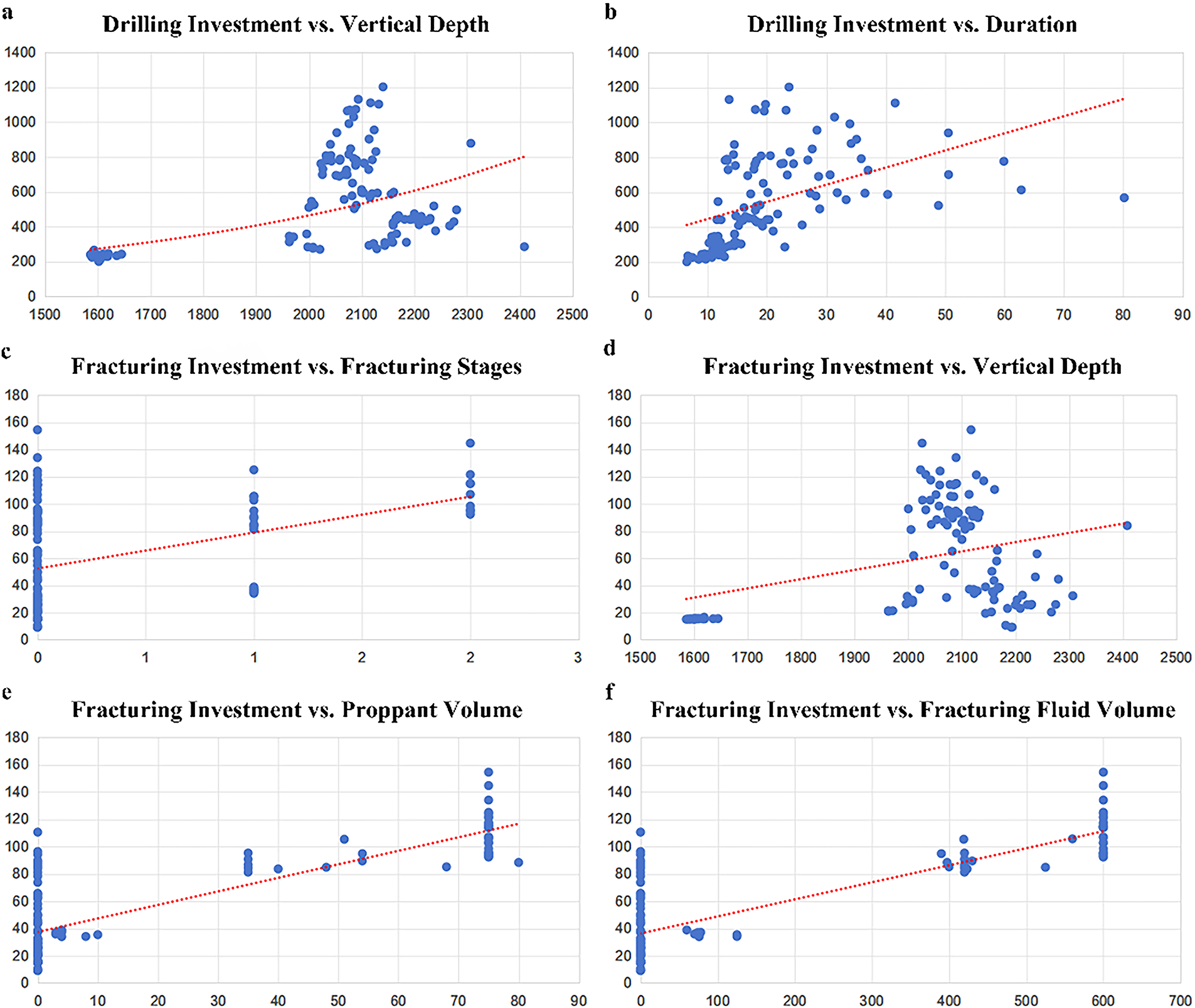
Figure 10: Single-Parameter fitting results of (a) drilling investment (10k CNY) vs. vertical depth (m); (b) drilling investment (10k CNY) vs. Duration (day); (c) fracturing investment (10k CNY) vs. fracturing stages; (d) fracturing investment (10k CNY) vs. vertical depth (m); (e) fracturing investment (10k CNY) vs. proppant volume (m3); (f) fracturing investment (10k CNY) vs. fracturing fluid volume (m3)
The correlation test results are presented in Fig. 11a,b. Drilling investment shows significant linear and monotonic relationships with construction period and vertical depth, while fracturing investment exhibits significant linear correlations with vertical depth, fracturing stages, fracturing fluid volume, and proppant volume.
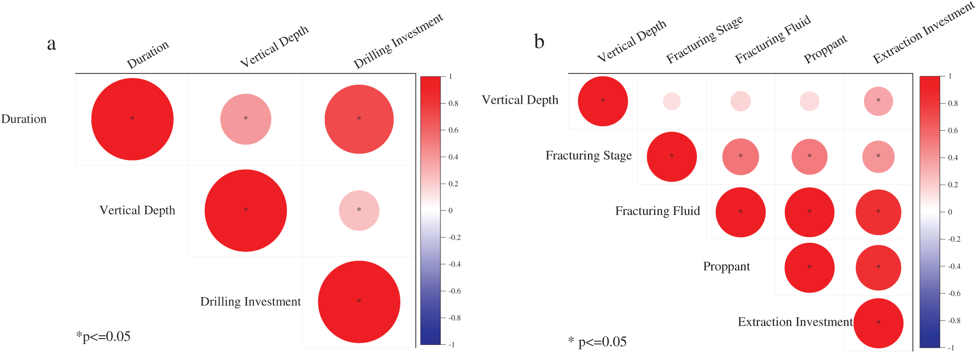
Figure 11: Correlation test of (a) drilling investment; (b) fracturing investment
Fig. 12a,b presents the multivariate regression fitting results for drilling and fracturing investments, respectively. Since multivariate fitting cannot visually depict the relationships between multiple independent variables and the response variable simultaneously, the x-axis displays individual well data points, while the y-axis represents the corresponding well investments. Both drilling and fracturing investment data were randomly divided into training (>80%) and test sets. The multivariate model developed from the training set was then used to predict the test set data, thereby validating the regression results.
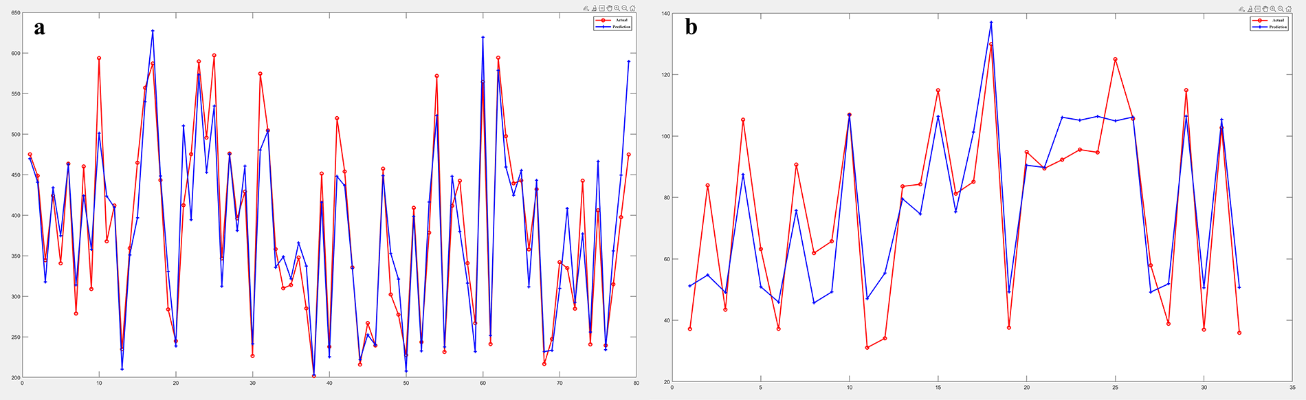
Figure 12: Model predictions vs. actual results comparison chart of (a) drilling investment (10k CNY); (b) fracturing investment (10k CNY)
The drilling investment model achieved R2 values of 0.87 for both the training and test sets, while the fracturing investment model attained R2 values of 0.81 for the training set and 0.77 for the test set, indicating strong explanatory power over the actual data. Notably, the models demonstrate robust predictive capability despite the presence of extreme outliers clustered above and below the average values in the plot.
The drilling investment function reveals a power relationship with vertical depth:
where
Fracturing investment shows linear relationships with engineering parameters:
where
Surface facility investment uses a mean value of 138 for this reservoir type, with the values in parentheses indicating the investment range (10–491) within the block.
Fig. 13a,b respectively present total investment plotted against individual engineering parameters. Due to the high goodness of fit, these plots were generated using regression functions, with the remaining parameters held constant at their mean values for the reservoir type.
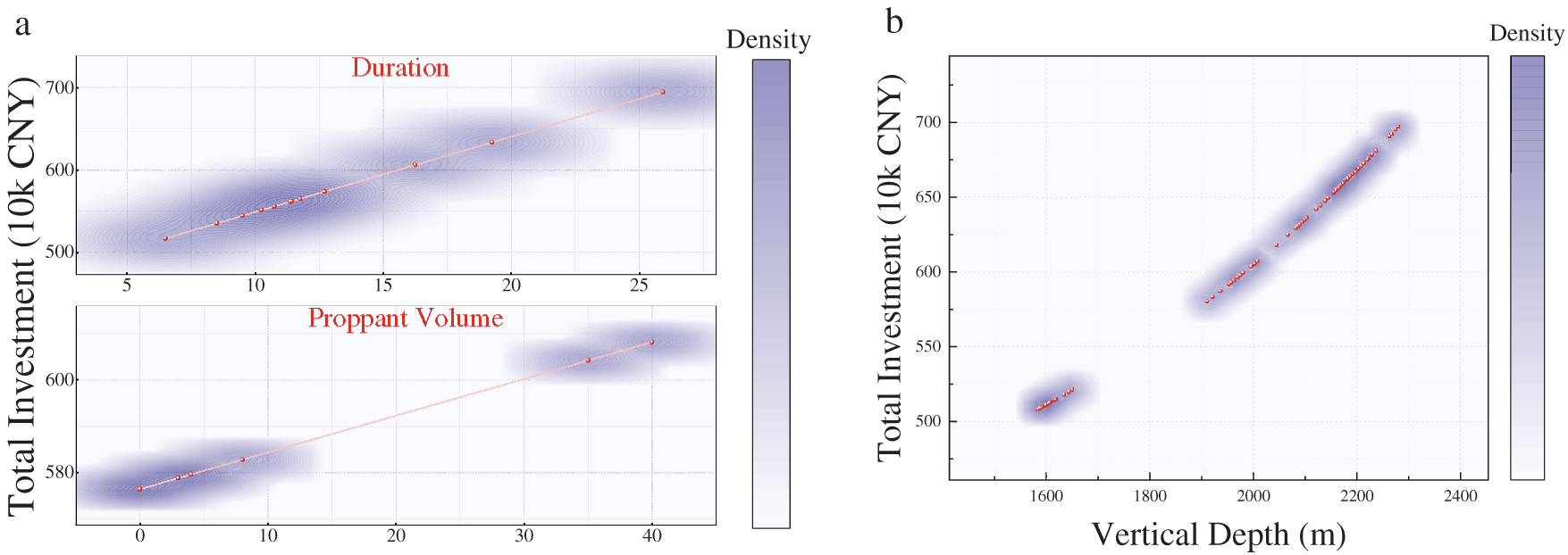
Figure 13: Univariate relationship diagrams of total investment with (a) duration (day) and proppant volume (m3); (b) vertical depth (m)
The analysis reveals significant correlations between investment and three key parameters: construction period, proppant volume, and vertical depth. Notably, total investment increases substantially when the vertical depth exceeds 2000 m. The distributions of proppant volume and vertical depth are primarily concentrated at the lower and upper extremes of their respective data ranges.
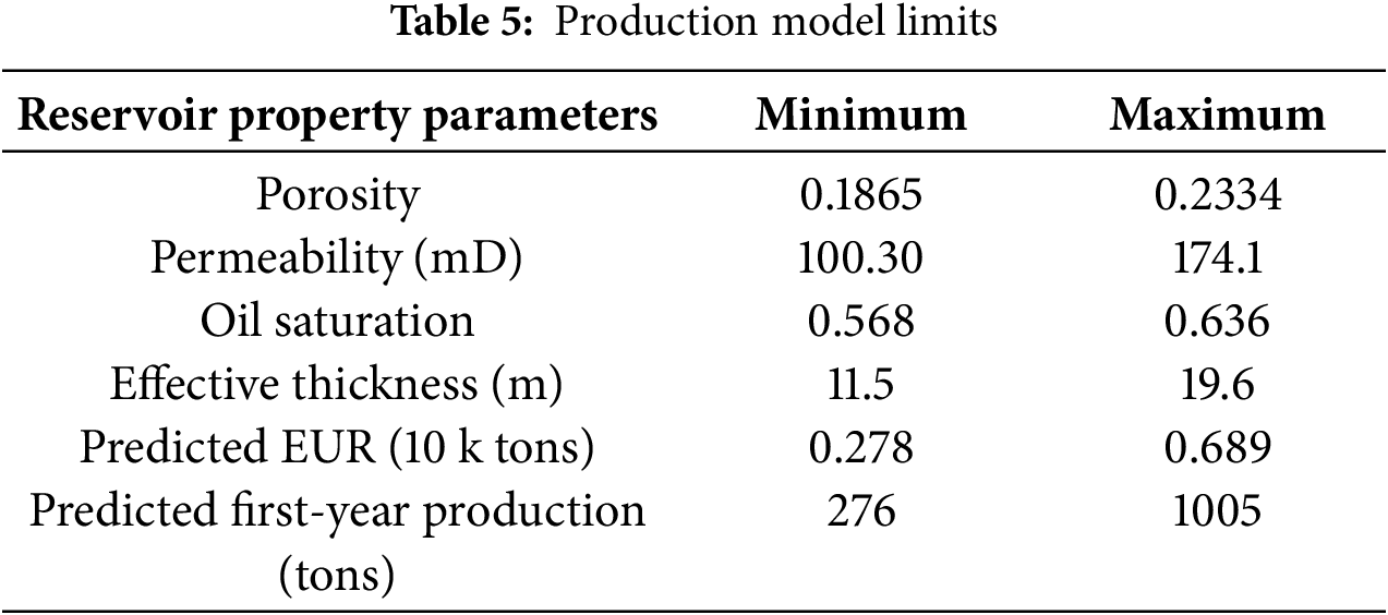
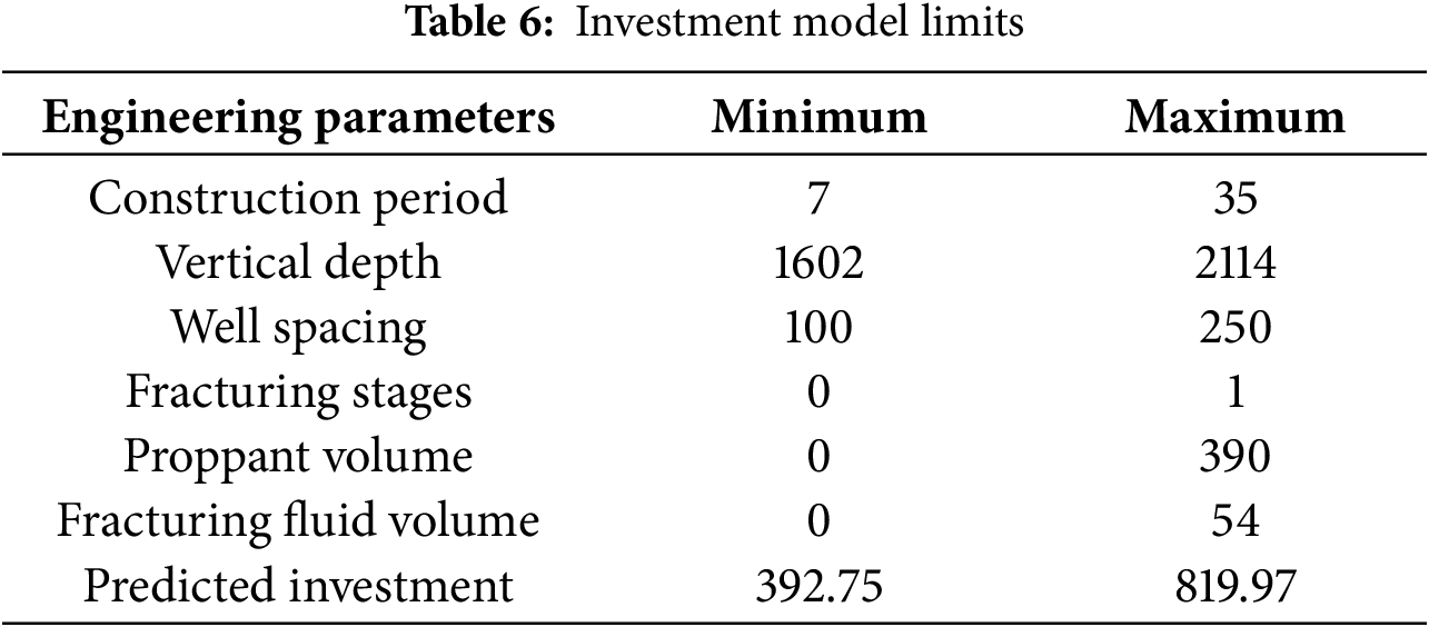
The data ranges were defined based on production and investment models for each reservoir type and development strategy, along with their key controlling parameters. Table 5 summarizes the limits of the production model. For this reservoir type, the ranges of porosity, permeability, oil saturation, and effective thickness are 0.18–0.23, 100.3–174.1 mD, 0.57–0.64, and 11.5–19.6 m, respectively. Table 6 specifies the investment model limits, where the ranges for construction period, vertical depth, well spacing, fracturing stages, fracturing fluid volume, and proppant volume are 7–35 days, 1602–2114 m, 100–250 m, 0–1, 0–390 m3, and 0–54 m3, respectively.
The number of new wells was set to 1, with a discount rate of 8%, an exchange rate of 6.9, and a depreciation period of 15 years. These parameters were used to construct the techno-economic boundary model charts.
4.3.2 Fundamental Economic Evaluation Model Charts
The break-even investment vs. cumulative production charts are shown in Fig. 14a,b. The x-axis represents cumulative production (10k tons), and the y-axis indicates break-even investment (10k CNY). Colored lines correspond to oil prices ranging from 40 to 90 USD/bbl. As illustrated, input well-group values (triangle markers) lie below the 60 USD/bbl line but above the 50 USD/bbl line, indicating that under the given parameter settings, IRR exceeds 8% when oil prices surpass 50 USD/bbl.
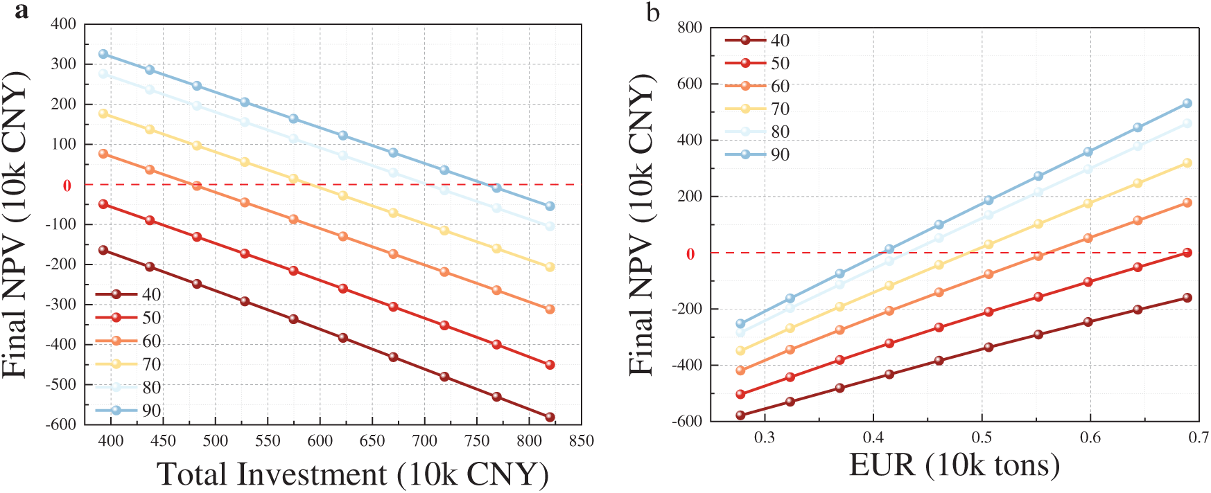
Figure 14: Plots of NPV with (a) EUR; (b) total investment
NPV charts illustrate how NPV varies with total investment and cumulative production under different oil price scenarios. In the NPV vs. total investment model, the EUR was fixed at the average value for this reservoir type. Conversely, in the NPV vs. EUR model, the total investment was set to the average for this reservoir type.
4.3.3 Techno-Economic Boundary Model Chart
Based on the established economic model, break-even cumulative production charts were developed under varying oil price scenarios (Fig. 15a,b). These charts delineate threshold cumulative production values within the investment range for this reservoir type, where data points below the gradient lines indicate economic non-viability at the corresponding oil prices.
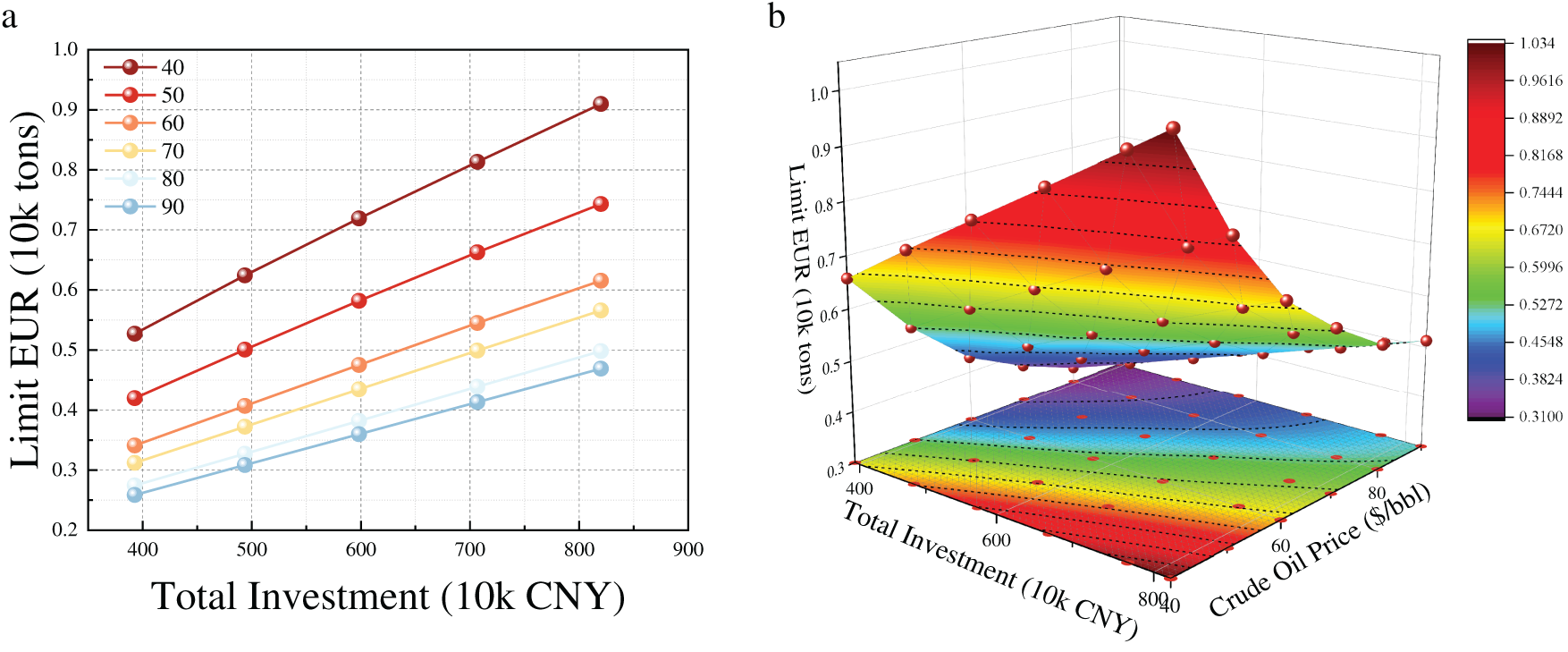
Figure 15: Plots of limit EUR with total investment: (a). 2D chart; (b). 3D heat map
The break-even cumulative production vs. engineering parameter charts consist of two types: break-even cumulative production vs. vertical depth relationships (Fig. 16a,b) and break-even cumulative production vs. construction period relationships (Fig. 17a,b).
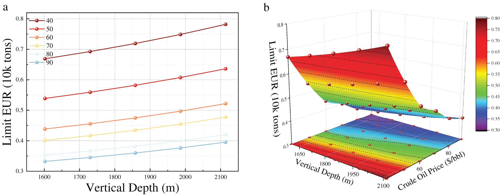
Figure 16: Plots of limit EUR with vertical depth: (a). 2D chart; (b). 3D heat map
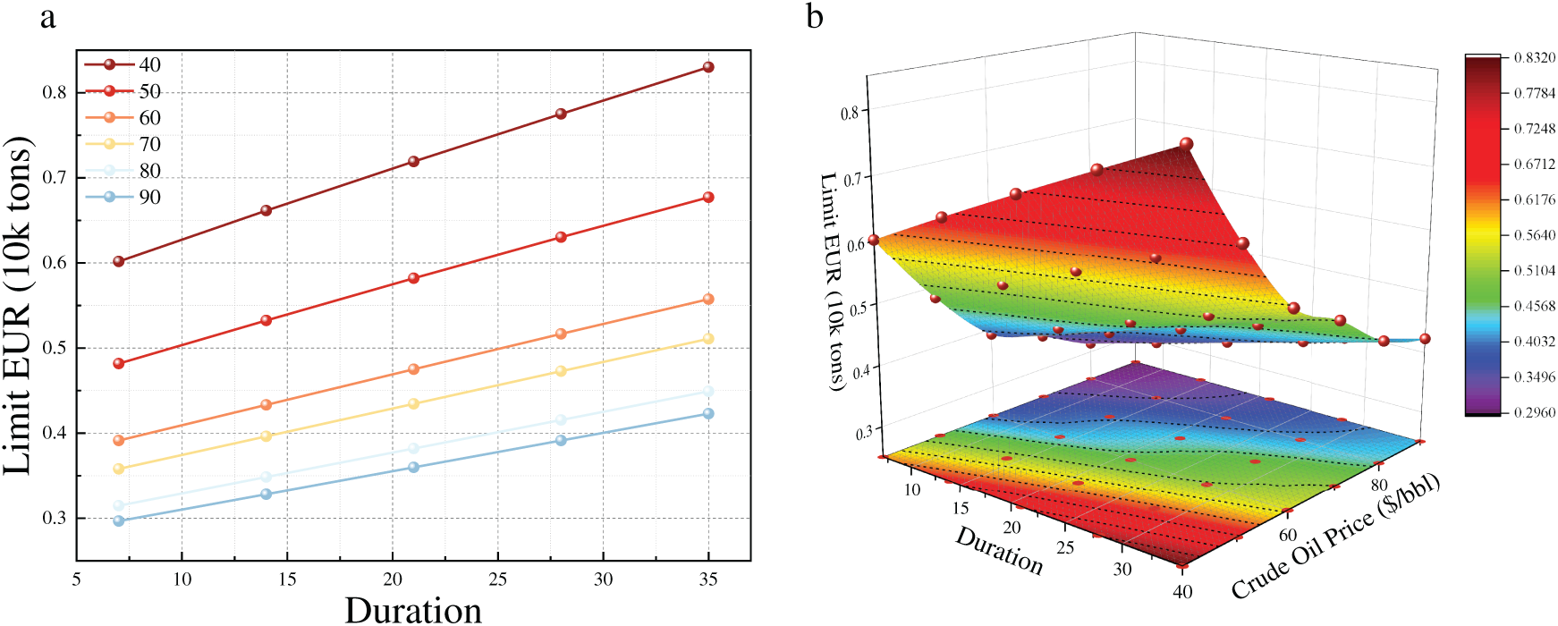
Figure 17: Plots of limit EUR with duration: (a). 2D chart; (b). 3D heat map
Complementarily, break-even investment charts were generated (Fig. 18a,b), with values above the gradient lines indicating economic infeasibility. Break-even investment vs. reservoir property charts include break-even investment vs. effective thickness (Fig. 19a,b) and break-even investment vs. oil saturation (Fig. 20a,b).
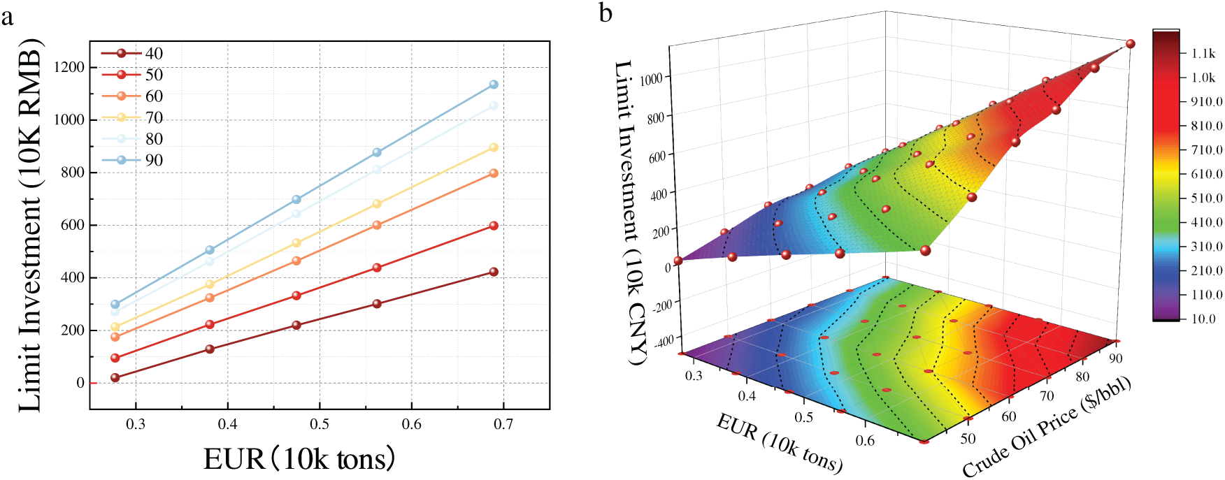
Figure 18: Plots of limit investment with EUR: (a). 2D chart; (b). 3D heat map
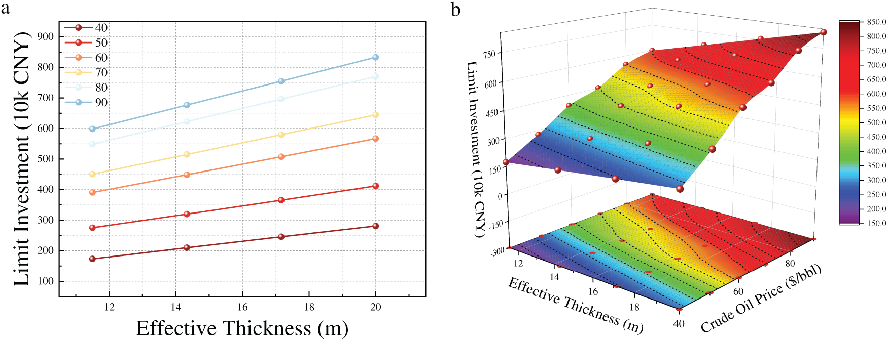
Figure 19: Plots of limit investment with effective thickness: (a). 2D chart; (b). 3D heat map
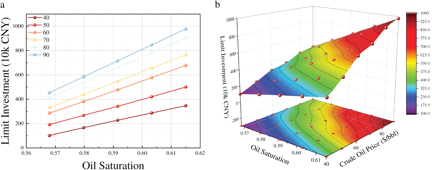
Figure 20: Plots of limit investment with oil saturation: (a). 2D chart; (b). 3D heat map
The integrated break-even analysis model determines the minimum economic thickness threshold (Fig. 21) for oil prices ranging from 40 to 90 USD/bbl. Investment was fixed at the reservoir-type average, while non-thickness reservoir properties were held at block averages. As illustrated in the figure, when oil prices increase from 40 to 90 USD/bbl, the minimum economic thickness threshold decreases from approximately 5.7 m to about 2.5 m, demonstrating the corresponding commercial viability of oil layer thickness in medium-permeability sandstone reservoirs under varying oil price conditions.
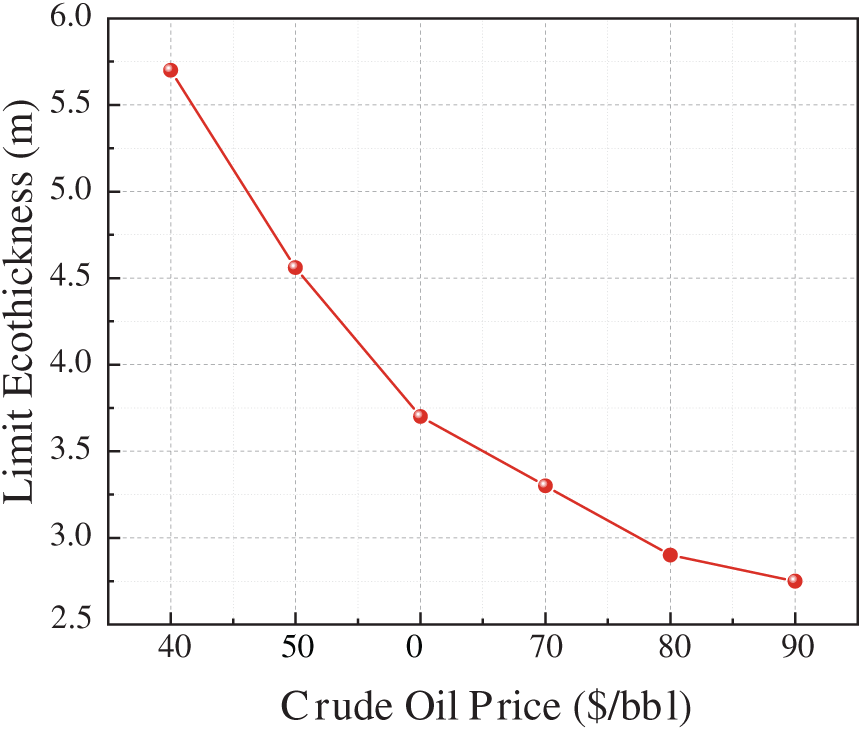
Figure 21: Minimum economic thickness threshold
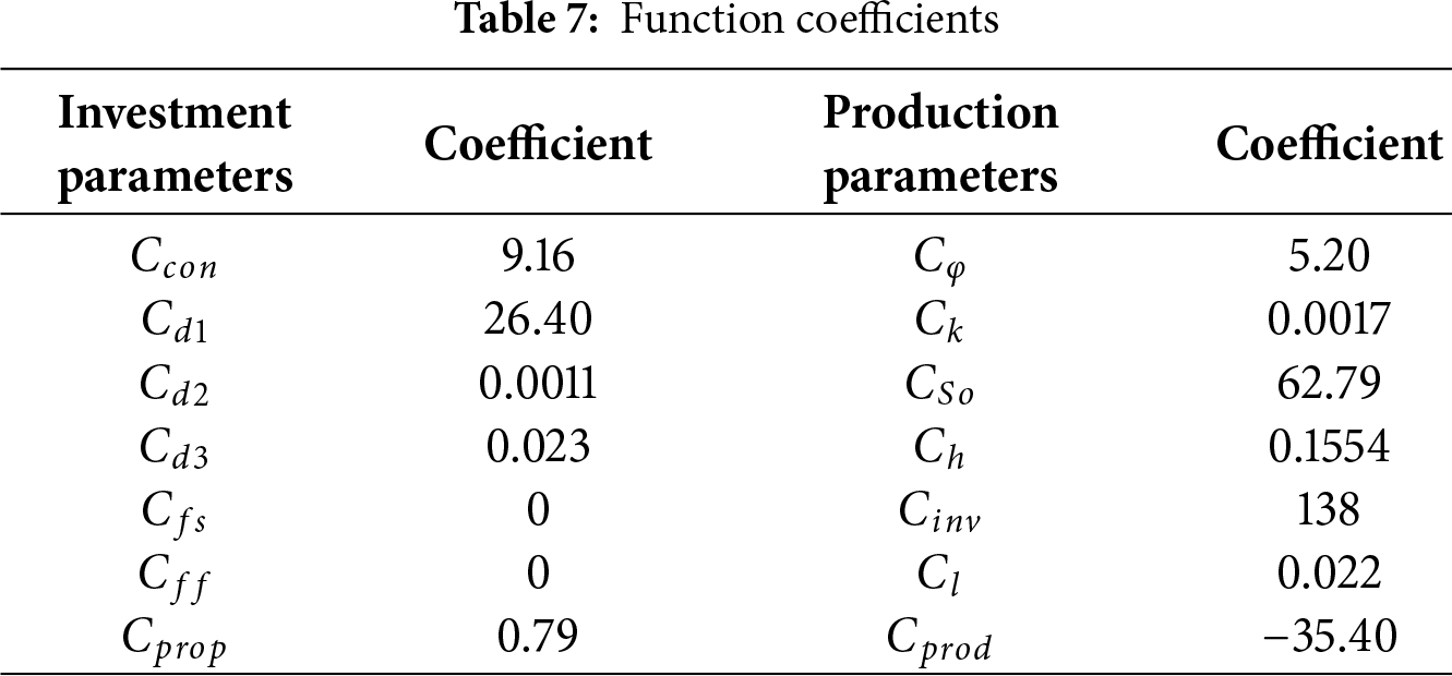
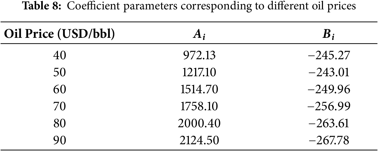
The break-even investment-cumulative production relationship at 8% IRR across oil prices is expressed as:
where
Among these, the coefficients in the investment and cumulative production functions are shown in Table 7, while the coefficients corresponding to different oil prices are presented in Table 8.
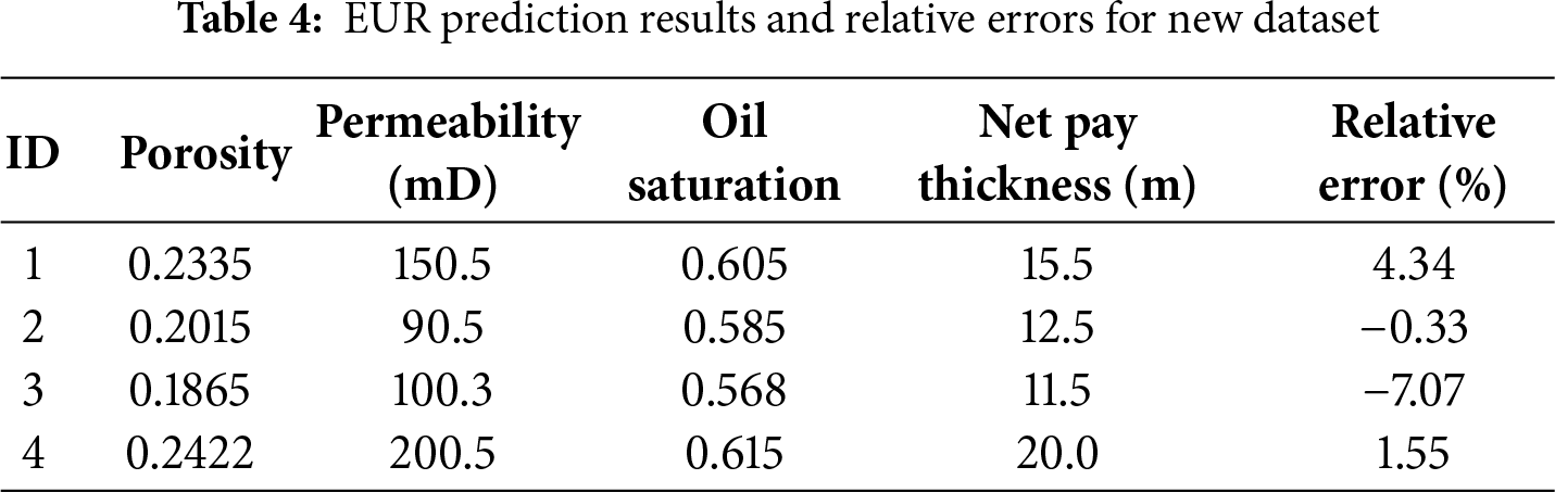
Validation with new datasets confirmed the predictive accuracy of the economic charts, demonstrating less than 25% relative error in the model projections. These results provide actionable guidance for the development planning of undeveloped reservoirs.
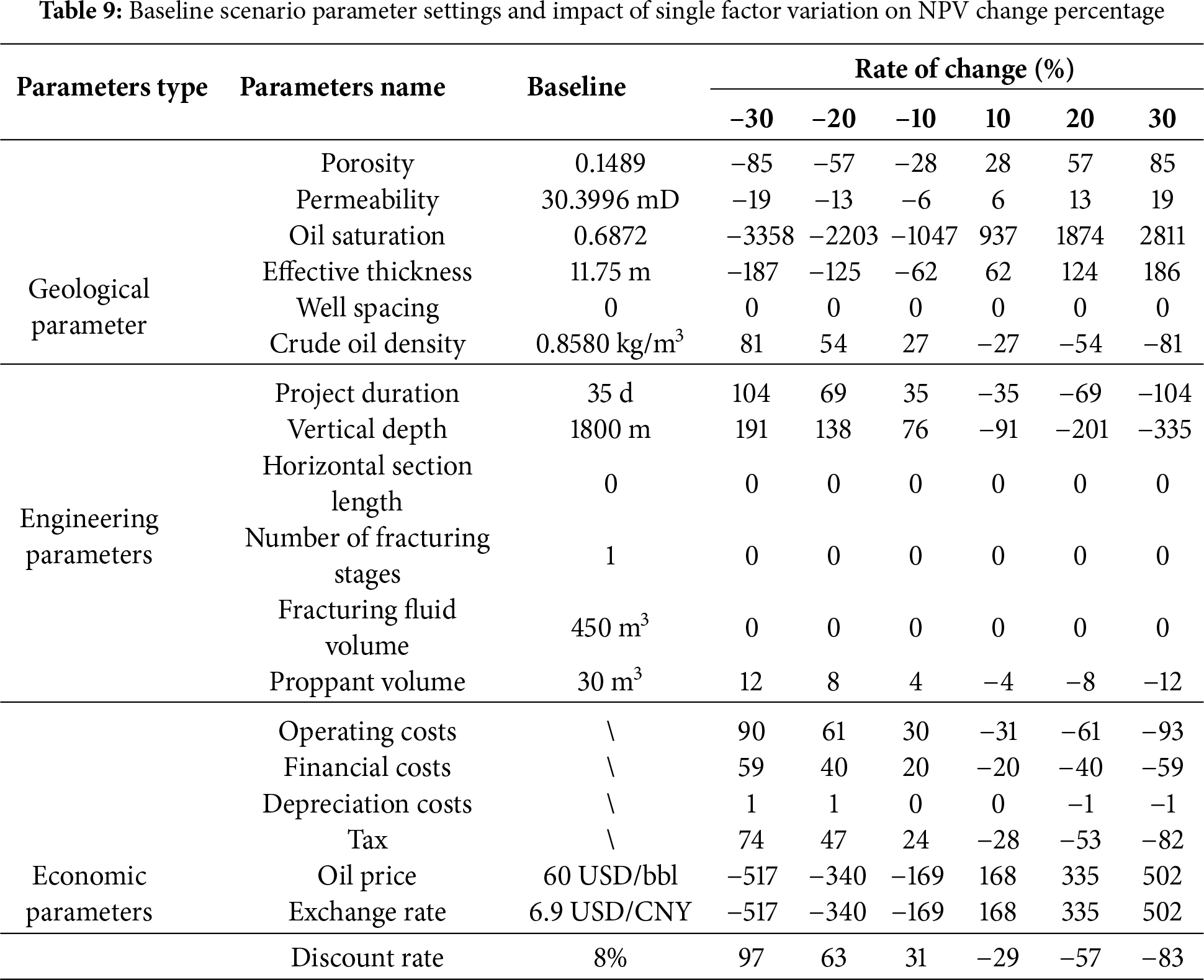
To systematically identify the key risk factors influencing the economic benefits of oilfield development, this study conducted a sensitivity analysis to evaluate the impact of geological, engineering, and economic parameters on NPV within a ±30% variation range. The analysis employed a single-factor variation method, in which only one parameter was altered at a time from the baseline scenario while observing the relative percentage change in NPV. The baseline scenario parameter settings and detailed results are presented in Table 9.
By calculating the average sensitivity coefficients of various parameters, this study quantified the impact of different factors on economic benefits. Fig. 22a–c displays the sensitivity curves for the three parameter categories, visually illustrating the functional relationship between parameter variations and NPV responses. Fig. 23a–c respectively present the sensitivity rankings of geological, engineering, and economic parameters using tornado diagrams. Additionally, Fig. 24 highlights the tornado diagram of parameters with high sensitivity coefficients, providing a focused perspective for identifying key risk factors.
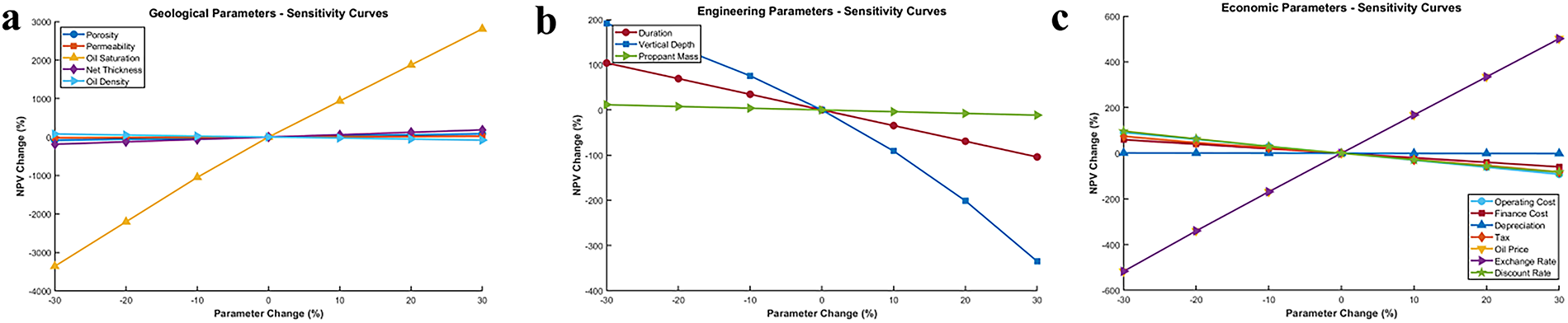
Figure 22: Sensitivity curves of (a) geological parameters; (b) engineering parameters; (c) economic parameters
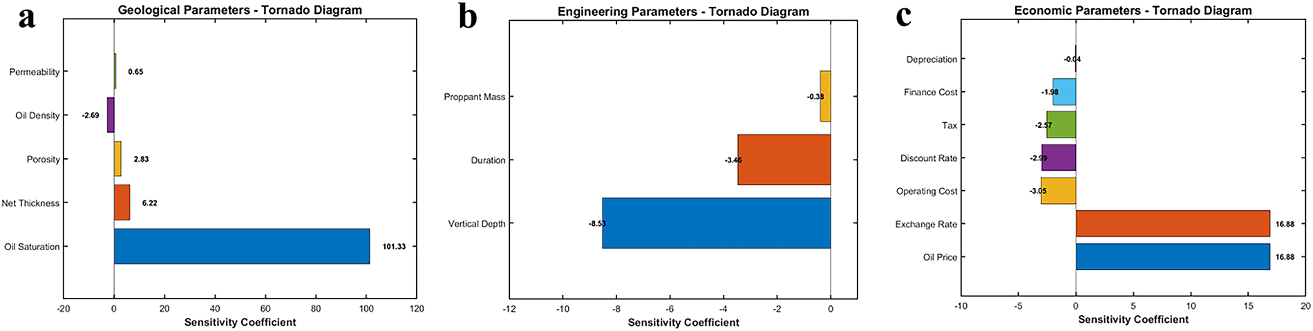
Figure 23: Sensitivity coefficient tornado diagrams of (a) geological parameters; (b) engineering parameters; (c) economic parameters
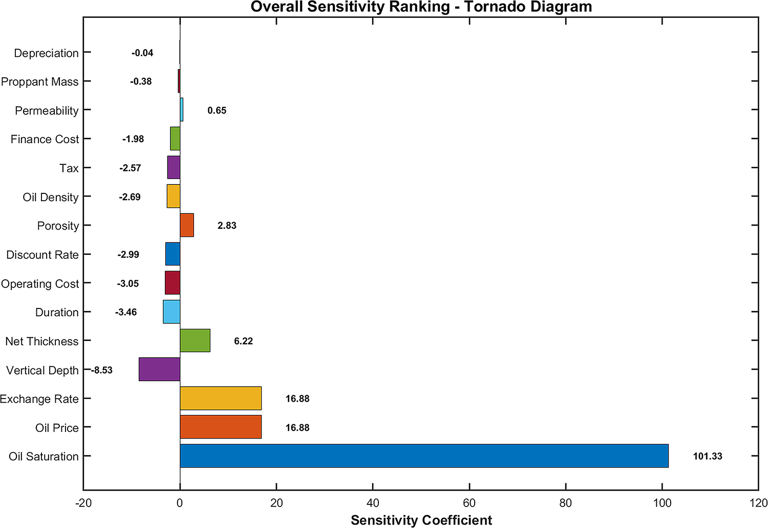
Figure 24: Tornado diagram of parameters with high sensitivity coefficients
The analysis results indicate that among geological parameters, oil saturation has the most significant impact, with a sensitivity coefficient as high as 101.33, underscoring its decisive role in the project’s economic benefits. Effective thickness follows, with a sensitivity coefficient of 6.22, indicating moderate sensitivity. For engineering parameters, vertical depth (sensitivity coefficient of −8.53) and project duration (sensitivity coefficient of −3.46) were identified as key influencing factors, both negatively correlated with investment costs. Among economic parameters, oil price and exchange rate each have sensitivity coefficients of 16.88, significantly higher than those of other parameters, highlighting the substantial impact of the external market environment on the project’s economic benefits.
Notably, certain parameters—such as well spacing, horizontal section length, number of fracturing stages, and fracturing fluid volume—showed no significant impact on NPV within the analyzed range, offering valuable insights for optimizing development plans. The study also revealed clear nonlinear relationships between variations in highly sensitive parameters and NPV responses, with the magnitude of NPV growth during positive parameter changes generally exceeding the magnitude of decline during negative changes.
This sensitivity analysis provides a scientific basis for managing risks in oilfield development. It is recommended to focus on monitoring high-sensitivity parameters such as oil saturation, oil price, and exchange rate, and to manage related risks through refined geological research and the application of financial instruments. For medium-sensitivity parameters, such as effective thickness and vertical depth, these should be fully considered in development plan optimization, with efforts to control their uncertainty impacts through technological advancements and engineering optimization. The research results are not only applicable to medium-permeability sandstone reservoirs in the Xinjiang Oilfield but also offer a methodological reference for the economic evaluation of other types of oil and gas reservoirs.
This study investigated the techno-economic limits of undeveloped reservoirs using an integrated methodological approach. For production forecasting, a heterogeneous numerical simulation model was developed for medium-permeability sandstone reservoirs under inverted seven-spot waterflood development. Historical matching with actual production data from representative well groups validated the model’s accuracy. Subsequent ten-year production forecasts closely aligned with field observations, confirming the suitability of numerical simulation for forecasting production in undeveloped reservoirs. Additionally, a multiple linear regression model for estimating EUR was developed using least squares fitting, achieving prediction relative errors below 25% on new datasets, indicating high predictive reliability.
Regarding investment estimation, multivariate regression models were developed for vertical wells in waterflooded sandstone formations. These models quantified explicit mathematical relationships between drilling and production investments and explanatory variables, enabling accurate cost predictions across various development scenarios. Complementary cost valuation frameworks were established through systematic analysis of operational expenditures throughout hydrocarbon production processes, providing a foundation for categorized cost estimation.
For techno-economic boundary modeling, NPV and IRR calculations were used to assess the current investment value. Dynamic economic evaluation charts were created for multiple oil price scenarios, including EUR-NPV, Investment-NPV, EUR-IRR, and Investment-IRR templates. These visualization tools clearly demonstrate how NPV and IRR respond to changes in investment and production under varying oil prices, facilitating rapid decision-making support.
Additionally, a break-even analysis was conducted to determine economic thresholds. Charts illustrating break-even cumulative production vs. investment, limit investment vs. cumulative production, and economic limit templates were generated. These visualizations clarify the relationships between cumulative production and investment at break-even points across different oil price regimes, effectively demonstrating the impact of oil price volatility on development economics. Furthermore, a single-factor sensitivity analysis was performed. The results indicated that oil saturation content had the greatest impact on NPV, followed by oil price, exchange rate, and well depth.
In summary, this research makes significant advancements in defining the techno-economic boundaries of undeveloped reservoirs. The developed production forecasting models, investment estimation frameworks, and economic boundary visualization systems provide a scientific foundation for oilfield development investment decisions. These contributions not only improve the economic performance of oilfield operators but also play a crucial role in safeguarding national and regional energy security. Future work will focus on advancing exploitation technologies for undeveloped reserves, thereby supporting the high-quality development of petroleum industry.
This study has certain limitations that also highlight directions for future research. Although the regression models demonstrate a good fit, they are based on a specific dataset, and their generalizability to other geological settings should be validated with additional data. The economic evaluation is primarily deterministic; incorporating probabilistic analysis would further enhance its robustness. Finally, the framework focuses on medium-permeability sandstone reservoirs; adapting it to other reservoir types (e.g., low-permeability formations or heavy oil reservoirs) would require recalibration of the production and investment models.
Acknowledgement: The authors gratefully acknowledge China National Petroleum Corporation (CNPC) for providing critical research data for this study.
Funding Statement: The authors received no specific funding for this study.
Author Contributions: The authors confirm contribution to the paper as follows: Conceptualization, Man Zhang and Cheng Chen; methodology, Cheng Chen; software, Hai-Xia Guo; validation, Man Zhang, Cheng Chen and Hai-Xia Guo; formal analysis, Xin-Jian Zhao; investigation, Hai-Xia Guo; resources, Man Zhang; data curation, Man Zhang; writing—original draft preparation, Xin-Jian Zhao; writing—review and editing, Man Zhang; visualization, Yi-Ming Xiao; supervision, Man Zhang; project administration, Cheng Chen. All authors reviewed the results and approved the final version of the manuscript.
Availability of Data and Materials: Not applicable.
Ethics Approval: Not applicable.
Conflicts of Interest: The authors declare no conflicts of interest to report regarding the present study.
Glossary
| Estimated Ultimate Recover (EUR) | The total amount of oil or gas expected to be recoverable from a reservoir over its lifetime |
| Latin Hypercube Sampling (LHS) | A statistical sampling method for stratified random sampling in multiple dimensions |
| Net Present Value (NPV) | The difference between present value of cash inflows and outflows over a period |
| Break-Even Point (BEP) | The production level where total revenue equals total costs |
| Water Cut | The ratio of water produced compared to the total volume of fluids |
| Discounted Cash Flow (DCF) | Financial analysis method evaluating project profitability |
| Enhanced Oil Recovery (EOR) | Techniques to increase oil extraction beyond primary methods |
| Liquefied Petroleum Gas (LPG) | Flammable hydrocarbon gas mixture used as fuel |
| West Texas Intermediate (WTI) | Benchmark crude oil price reference |
| Internal Rate of Return (IRR) | Discount rate where NPV equals zero |
| Fully Allocated Cost (FAC) | Total cost per unit of production including all expenses |
| Break-Even Point (BEP) | Production level where revenue equals costs |
| Value Added Tax (VAT) | Consumption tax on value added at production stages |
References
1. IEA. Oil 2023 [Internet]. Paris, France: International Energy Agency; 2023 [cited 2025 Aug 14]. Available from: https://www.iea.org/reports/oil-2023. [Google Scholar]
2. Nandi BK, Kabir MH, Nandi MK. Crude oil price hikes and exchange rate volatility: a lesson from the Bangladesh economy. Resour Policy. 2024;91(2):104858. doi:10.1016/j.resourpol.2024.104858. [Google Scholar] [CrossRef]
3. Popescu C, Gheorghiu SA. Economic analysis and generic algorithm for optimizing the investments decision-making process in oil field development. Energies. 2021;14(19):6119. doi:10.3390/en14196119. [Google Scholar] [CrossRef]
4. Wang JQ, Shi CF, Ji SH. New water drive characteristic curves at ultra-high water cut stage. Pet Explor Dev. 2017;44(6):955–60. doi:10.1016/S1876-3804(17)30113-1. [Google Scholar] [CrossRef]
5. Liu F, Liu Y, Guo X, Yang F, Zhou A, Li C. A new growth curve for predicting production performance of water-flooding oilfields. Math Probl Eng. 2021;2021(3):7787850. doi:10.1155/2021/7787850. [Google Scholar] [CrossRef]
6. Dou HE, Zhang HJ, Shen SB. Correct understanding and application of water flooding characteristic curve. Pet Explor Dev. 2019;46(4):755–62. doi:10.1016/S1876-3804(19)60237-5. [Google Scholar] [CrossRef]
7. Kaiser MJ. Hydrocarbon production forecast for Louisiana-Producing field module. Math Comput Model. 2012;55(3–4):564–89. doi:10.1016/j.mcm.2011.08.028. [Google Scholar] [CrossRef]
8. Makinde I, Lee WJ. Forecasting production of liquid rich shale (LRS) reservoirs using simple models. J Pet Sci Eng. 2017;157:461–81. doi:10.1016/j.petrol.2017.04.038. [Google Scholar] [CrossRef]
9. Feng Q, Wu K, Zhang J, Wang S, Zhang X, Zhou D, et al. Optimization of well control during gas flooding using the deep-LSTM-based proxy model: a case study in the Baoshaceng reservoir, Tarim, China. Energies. 2022;15(7):2398. doi:10.3390/en15072398. [Google Scholar] [CrossRef]
10. Redutskiy Y. Integration of oilfield planning problems: infrastructure design, development planning and production scheduling. J Pet Sci Eng. 2017;158:585–602. doi:10.1016/j.petrol.2017.08.066. [Google Scholar] [CrossRef]
11. Wang T, Liu F, Li X. Optimization of efficient development modes of offshore heavy oil and development planning of potential reserves in China. Water. 2023;15(10):1897. doi:10.3390/w15101897. [Google Scholar] [CrossRef]
12. Yang T, Liang Y, Wang Z, Ji Q. Dynamic prediction of shale gas drilling costs based on machine learning. Appl Sci. 2024;14(23):10984. doi:10.3390/app142310984. [Google Scholar] [CrossRef]
13. Zhu H. Method for determining lowest oil price limit by developing tight peripheral oil in Daqing. IOP Conf Ser Earth Environ Sci. 2021;632(2):022011. doi:10.1088/1755-1315/632/2/022011. [Google Scholar] [CrossRef]
14. Jang D, Kim K, Kim KH, Kang S. Techno-economic analysis and Monte Carlo simulation for green hydrogen production using offshore wind power plant. Energy Convers Manag. 2022;263:115695. doi:10.1016/j.enconman.2022.115695. [Google Scholar] [CrossRef]
15. Abbas AJ, Gzar HA, Rahi MN. Oilfield-produced water characteristics and treatment technologies: a mini review. IOP Conf Ser Mater Sci Eng. 2021;1058(1):012063. doi:10.1088/1757-899X/1058/1/012063. [Google Scholar] [CrossRef]
16. Armoo EA, Mohammed M, Narra S, Beguedou E, Agyenim FB, Kemausuor F. Achieving Techno-economic feasibility for hybrid renewable energy systems through the production of energy and alternative fuels. Energies. 2024;17(3):735. doi:10.3390/en17030735. [Google Scholar] [CrossRef]
17. Li J, Wu T, Lu Z, Wu S. Investigation into mining economic evaluation approaches based on the rosenblueth point estimate method. Appl Sci. 2023;13(15):9011. doi:10.3390/app13159011. [Google Scholar] [CrossRef]
18. Arps JJ. Analysis of decline curves. Trans AIME. 1945;160:228–47. doi:10.2118/945228-G. [Google Scholar] [CrossRef]
19. Sharma A, Lee WJ. Improved workflow for EUR prediction in unconventional reservoirs. In: Proceedings of the SEG Global Meeting Abstracts; 2016 Oct 16–21; Dallas, TX, USA. p. 961–78. doi:10.15530/urtec-2016-244428. [Google Scholar] [CrossRef]
20. Wu J, Zhang L, Liu Y, Ma K, Luo X. Effect of displacement pressure gradient on oil-water relative permeability: experiment, correction method, and numerical simulation. Processes. 2024;12(2):330. doi:10.3390/pr12020330. [Google Scholar] [CrossRef]
21. Sikanyika EW, Wu Z, Mbarouk MS, Mafimba AM, Elbaloula HA, Jiang S. Numerical simulation of the oil production performance of different well patterns with water injection. Energies. 2023;16(1):91. doi:10.3390/en16010091. [Google Scholar] [CrossRef]
22. Shi MY, Wang JJ, Yi CG, Cheng R, He YY. Study of Forecasting and estimation methodology of oilfield development cost based on machine learning. Chem Technol Fuels Oils. 2021;56(6):1000–19. doi:10.1007/s10553-021-01217-y. [Google Scholar] [CrossRef]
23. Chen C, Liu Y, Lin D, Qu G, Zhi J, Liang S, et al. Research progress of oilfield development index prediction based on artificial neural networks. Energies. 2021;14(18):5844. doi:10.3390/en14185844. [Google Scholar] [CrossRef]
Cite This Article
 Copyright © 2026 The Author(s). Published by Tech Science Press.
This work is licensed under a Creative Commons Attribution 4.0 International License , which permits unrestricted use, distribution, and reproduction in any medium, provided the original work is properly cited.
 Downloads
 Citation Tools