Transient Voltage Control for AC-DC Hybrid Power System Based on ISAO-CNN-BiGRU

1  Introduction

In recent years, the increasing scale of interconnected power systems and the concentrated commissioning of high-voltage direct current (HVDC) transmission projects have brought the issue of transient voltage stability in hybrid AC/DC systems to the forefront [1–3]. Accurately assessing and controlling transient voltage stability following faults has consequently become a significant research focus. Concurrently, the growing complexity of hybrid AC/DC grid structures and the rising proportion of HVDC transmission capacity make it challenging for AC systems to maintain reactive power balance after major disturbances, potentially leading to sustained voltage depression or even collapse. Therefore, establishing an accurate method for transient voltage assessment and control is urgently needed, holding substantial practical significance and theoretical value for enhancing the secure and stable operation of hybrid AC/DC systems.

Conventional research on transient voltage stability assessment and control strategies typically employs time-domain simulation methods. These primarily analyze the transient voltage stability at load buses following significant disturbances. References [4,5] utilize time-domain simulation to analyze the evolution of transient voltages for different models. While time-domain simulation offers high precision, it requires lengthy computation times, making it difficult to meet the rapid response demands of modern power grids. With the rapid advancement of artificial intelligence (AI) techniques, researchers worldwide have applied AI to transient voltage stability assessment to address the limitations of time-domain simulation. AI methods generally establish a mapping relationship between input features and transient voltage stability by training on input datasets [6]. Current AI approaches for transient voltage stability include traditional artificial neural network (ANN) [7], support vector machine (SVM) [8], and decision tree (DT) [9].

Regarding neural networks themselves, convolutional neural network (CNN) have shown promising progress in assessing and controlling transient voltage stability in power systems [10]. Furthermore, combining CNNs with bidirectional gated recurrent unit network (BiGRU) efficiently processes time-series data with local characteristics, making it suitable for building response-driven models based on fused feature sets [11]. Although methods like CNN-BiGRU excel at processing temporal data, their performance and efficiency are inherently constrained by the quality and relevance of their input features. Many current approaches directly feed raw, high-dimensional electrical measurements into the model [12,13]. Although this strategy is logically sound, it often introduces a large number of irrelevant or redundant variables, which not only obscures the fundamental physical mechanisms driving instability but also increases the computational burden. Furthermore, the input feature data often fails to focus on critical instability regions, thereby limiting its potential for real-time applications. On the other hand, the complex structure of the CNN-BiGRU model makes its optimization process challenging. The previous trial and error method not only increased the optimization time, but also could not guarantee accuracy.

To address the aforementioned issues, this paper constructs a concise and efficient feature input set by screening characteristics that are strongly correlated with transient voltage instability and possess clear physical significance. Simultaneously, TVSI is introduced as a comprehensive metric to quantify the system’s post-disturbance transient voltage performance [14]. LVSI is defined as the ratio of the voltage change magnitude at a load node (or bus) to the change in the system-level TVSI, serving to accurately identify the response characteristics of critical load nodes. Furthermore, to tackle the challenges posed by the complex structure and difficult optimization of the CNN-BiGRU model, ISAO algorithm is employed to optimize the hyperparameters of CNN-BiGRU. Leveraging the powerful global search capability of ISAO [15], the optimal hyperparameter combination is sought to enhance the model’s prediction accuracy, accelerate the training convergence process, and ensure the real-time performance and reliability of the intelligent response. Therefore, the main contributions are:

1) Constructs a physics-informed “response-characteristic-driven” intelligent framework that achieves end-to-end output from post-fault feature extraction to synchronous generation of stability assessment and UVLS control strategies.

2) Introducing the LVSI to focus on critical instability regions, further enhancing the physical interpretability of the response-driven model and reducing the dimensionality of the input feature space.

3) Employing ISAO to globally optimize the key hyperparameters of the CNN-BiGRU network, overcoming the drawbacks of traditional trial-and-error methods, such as easily falling into local optima and high time consumption.

4) Comprehensively compare the proposed method with traditional artificial intelligence methods, classical reactive power compensation methods, and traditional UVLS schemes to verify its overall advantages in decision accuracy, speed, and robustness.

2  Composition of Input Set: Screening of Response Characteristic Data

According to “the technical specifications for safety and stability calculation of State Grid Corporation of China”, during a transient process, the load bus voltage must recover to above 0.80 p.u. after a fault. Following a disturbance in the power system, voltage conditions are generally categorized into four scenarios: voltage collapse, delayed voltage recovery, voltage-angle coupling instability, and sustained low voltage [16]. To address the issue of low-voltage instability in hybrid AC/DC power systems, several interpretable feature quantities that are strongly correlated with voltage stability are proposed to serve as the characteristic data for the input layer of the neural network.

2.1 Response Characteristic Data

2.1.1 P-I Change Rate

In hybrid AC/DC power systems, to achieve accurate identification of power supply-demand imbalance scenarios, the relationship between active power and current can be effectively utilized to identify the risk of transient voltage instability. When a load node experiences low-voltage instability, during the voltage descent process, the load node must inevitably remain in the voltage unstable region for a period of time. The load exhibits a contradictory characteristic of “increasing current but losing active power,” indicating that the load is attempting to draw more power by increasing current, but the actual power acquired decreases. This is a typical signature of voltage instability. Therefore, the voltage instability criterion is expressed as follows:

{Ik+1>Ik & Pk+1<PkIk+1−Ik>ε & Pk+1−Pk>εtk≥0.05 sVk<0.8(1)

where Ik, Pk is the current and active power at time k, Ik+1, Pk+1 is the current and active power at time k + 1, ε is a very small positive number, tk is the duration for which the criterion is satisfied, Vk is the voltage value after the end of the voltage decline.

As shown in Fig. 1, by comparing the variation trajectories of active power and current under post-fault voltage recovery to a stable state vs. voltage instability in the hybrid AC/DC system, it can be observed that when transient voltage instability occurs, the load exhibits the phenomenon of “increasing current but losing active power,” indicating its entry into the voltage unstable region.

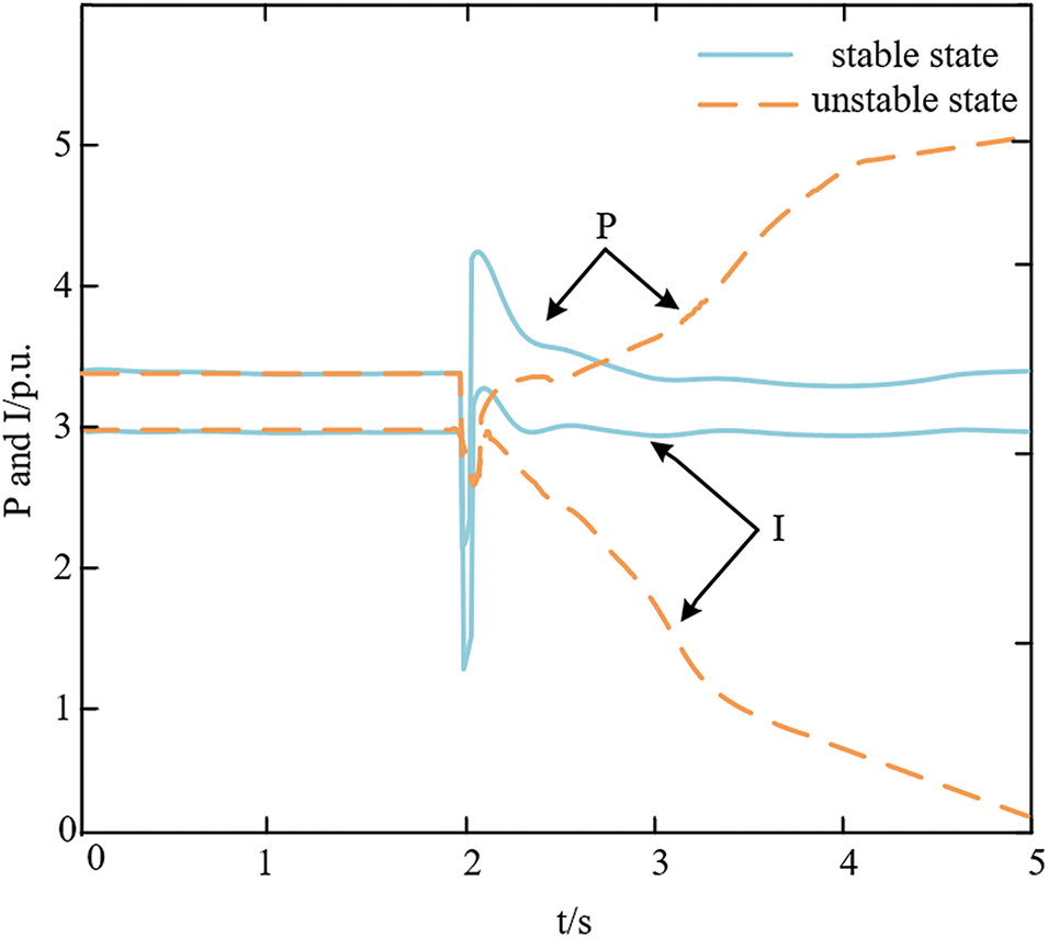
Figure 1: Active power and current under different conditions

The aforementioned voltage instability criterion, based on active power and current variations, enables the discrimination of voltage stability by capturing the system’s dynamic characteristics within the voltage unstable region. Therefore, the active power-current (P-I) change rate can also be expressed as:

dIdt⋅dPdt=(Ik+1−Ik)(Pk+1−Pk)<0(2)

Therefore, the P-I change rate is essentially a key state variable that quantifies whether a load node has entered the voltage unstable region. Usually, the active power and current values of the load within 0.2 s after the fault is resolved are selected, and their product is used as one of the characteristic data.

2.1.2 Integral Area Based on Voltage Trajectory

However, in scenarios involving severe system voltage sags under large disturbances, which lead to low-voltage instability caused by angle instability, the characteristics of the P-I change rate are not significant. Therefore, an integrated area based on voltage trajectories is introduced to represent such dynamic changes [17]. As shown in Fig. 2, during the voltage sag process, real-time integration is performed on the deviation from the specified 0.8 p.u., thereby obtaining the integrated area under unstable conditions.

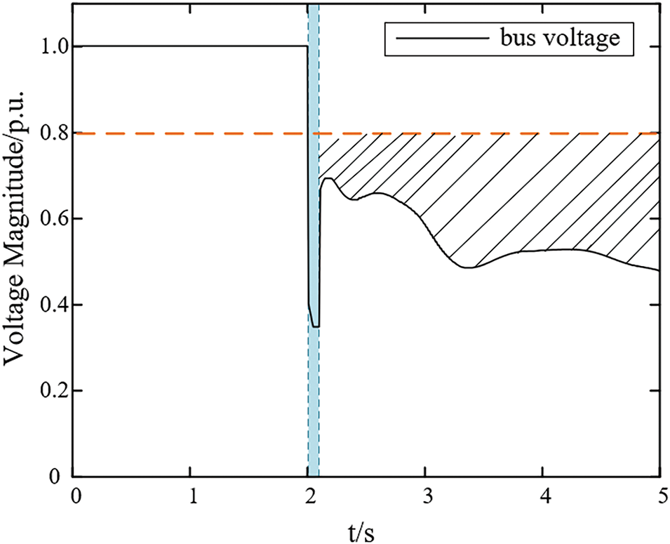
Figure 2: Disturbance voltage trajectory under voltage instability conditions

The corresponding expression, as shown in Eq. (3), not only represents the integrated area of the voltage trajectory but also considers the rate of voltage decline.

F=∫t0tz|V(s−T)−VsT|(Vh−Vs)ds(3)

where F is the integral area, Vh is the set value of the integral starting voltage, Vs is the voltage at time s, T is the sampling time interval, t0 is the integral starting time, tz is the integral termination time.

For stable conditions, when the voltage recovers above 0.8 p.u. and remains there for a certain period, the system is determined to be stable, and the integration process is reset, as illustrated in Fig. 3. For multi-swing processes, distinct features exist in the voltage trajectories, and the instability degree of the system during multi-swing is assessed through positive and negative integrated areas. Specifically, positive integration is applied before the trajectory inflection point, maintaining the original mapping relationship; negative integration is applied during the trajectory backswing, indicating a gradual reduction in the system’s transient instability degree, as depicted in Fig. 4.

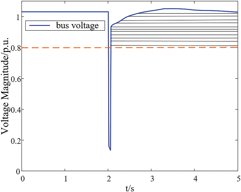
Figure 3: Disturbance voltage trajectory under voltage instability conditions

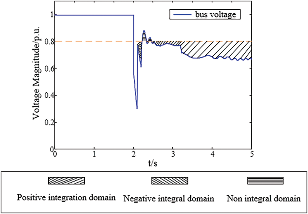
Figure 4: Schematic diagram of positive and negative integration during multi-swing

By selecting the voltage trajectory of the oscillation center and its adjacent key nodes for integral analysis, the transient voltage stability of the power system can be effectively determined to address the voltage stability/instability issues. The oscillation center of the system corresponds to the lowest point of the voltage in the system. By performing composite integration operations on the voltage trajectories of these key nodes, accurate evaluation of the transient stability of the entire network can be achieved. Therefore, this article proposes to achieve effective discrimination of system voltage stability by selecting the bus with the lowest voltage and its adjacent buses. The instability criteria used in this article are as follows:

F>Fset(4)

where Fset is the threshold value for integration.

In traditional methods, setting the integration threshold requires extensive simulation results based on various types of faults within the system. This involves obtaining post-disturbance voltage trajectories of key nodes and then setting respective integration thresholds capable of identifying system transient instability. To overcome the limitation of relying on manual experience, this paper uses the integrated trajectory area of bus voltage as a response feature data, and utilizes the powerful feature extraction ability of neural networks to adaptively determine potential threshold values, thereby reducing the subjectivity and engineering burden caused by manually setting thresholds.

2.1.3 Active Power at the Rectifier Side of the HVDC System

In hybrid AC/DC power systems, when a fault occurs in the AC system, it may affect the operation of the rectifier station in the high voltage direct current (HVDC) transmission system. When the AC system malfunctions and causes a transient voltage drop, the drop in the AC bus voltage of the rectifier station will directly affect its operating status. If the voltage drop is severe, it may cause the rectifier to block or commutation failure, resulting in the suspension of power transmission in the DC transmission system. At this point, the active power on the rectifier side will rapidly decrease to near zero. This sudden change disrupts the active power balance of the sending end system, especially when the receiving end is a load center or new energy base, which may cause frequency fluctuations and drastic changes in local voltage of the sending end system, thereby exacerbating the transient voltage instability process. Therefore, the drastic change in active power on the rectification side is not only a result of system faults, but also an important indicator signal of energy imbalance and stability deterioration during transient processes. It can be used as a key characteristic quantity to evaluate the dynamic behavior of the system and design control strategies. During normal HVDC operation, the active power at the rectifier side can be expressed as follows:

Pdc=UdcIdccos⁡θ(5)

where Pdc is the active power at the rectifier side, Idc is the current value at the rectifier side, Udc is the voltage value at the rectifier side, θ is the phase angle between voltage and current, which is typically 0 under ideal conditions.

When a fault occurs on the AC side leading to transient voltage instability, the transmission of active power at the rectifier side will be interrupted, i.e., the active power rapidly decays to zero or approaches zero. This process can be expressed as:

limt→tblockP(t)=limt→tblock[Udc(t)⋅Idc(t)]=0(6)

where tblock is the time instant at which DC blocking occurs.

Therefore, in the event of DC blocking or commutation failure faults, the active power at the rectifier side of the HVDC within 0.2 s after fault clearance is selected as part of the input set.

2.2 Screening of Key Characteristic Data

The extraction of the aforementioned key response characteristics has significantly reduced data redundancy. However, for large-scale power systems, their complex structure—involving numerous induction motors and load nodes—may still adversely impact the accuracy and efficiency of the response model. Therefore, LVSI is proposed to focus on critical instability regions and screen the characteristic quantities of load nodes that have a significant impact on the system’s transient voltage performance, thereby further optimizing the feature input set for driving intelligent response.

To assess the degree of transient voltage stability, TVSI is commonly used to quantify the transient voltage performance of system buses after fault clearance. It is expressed as follows:

TVSI=1N⋅∑i=1N|Vi−Vn|VnT−Tc(7)

where N is the total number of system buses, T is the duration of the transient analysis, TC is the fault occurrence time, Vn is the system rated voltage.

TVSI takes into account not only the magnitude of voltage deviation but also its duration, providing a more comprehensive reflection of the system’s voltage recovery performance during the transient process. This indicator is an average evaluation of the voltage performance of all busbars in the entire system, reflecting the overall transient voltage quality of the system.

To accurately identify key load nodes that significantly influence the system’s transient voltage stability, under the same fault condition, the relationship between a selected load node and the system-level TVSI is represented by the absolute ratio of the voltage change at an individual load bus to the change in TVSI, as shown in Eq. (8):

LVSI=|Vi,t−Vi,t−1||TVSIt−TVSIt−1|(8)

where Vi,t is the voltage of the i bus at time t.

The average LVSI value for the same load bus across the studied period is then calculated as:

LVSI¯=LVSI1+LVSI2+......+LVSInk(9)

where k is the time length from fault initiation to the end of transient analysis.

Below is a detailed introduction to the specific application of LVSI in this article. Firstly, analyze a voltage situation under a certain power flow situation, and obtain the system level TVSI values at each sampling time point after all bus faults in the system. Secondly, the absolute value of the difference between the voltage of the load node (or bus) at each sampling time point and the voltage of the load node (or bus) at the previous time point is taken as the numerator, and the absolute value of the difference between the TVSI at each sampling time point and the TVSI at the previous time point is taken as the denominator, which is defined as LVSI. Then calculate the average LVSI value of each load node (or bus) after the fault ends. Select load nodes (or buses) with higher LVSI values by comparing the average LVSI values obtained. Finally, count the load nodes (or buses) that have a significant impact on the transient voltage stability at the system level among the instability situations listed under each power flow. Select feature data related to load nodes (or buses) with higher LVSI values as the training set for the neural network, and discard load nodes (or buses) with lower LVSI values.

From this, it can be seen that LVSI quantifies the sensitivity of load bus voltage to transient voltage instability in the system. The higher the LVSI value, the greater the impact of the bus voltage fluctuation on the system level transient voltage stability, which is a key node that needs to be closely monitored; On the contrary, a lower LVSI value indicates that the node’s impact on system stability can be ignored. This is consistent with the physical characteristic that transient voltage instability often originates from localized load concentration areas and is accompanied by sustained voltage drops.

In summary, this chapter has successfully constructed an input feature dataset characterized by high relevance and low redundancy by introducing response characteristic quantities with clear physical significance and defining the LVSI index to screen key nodes. This dataset provides a solid foundation for the subsequent construction of an intelligent response model, effectively addressing issues in traditional methods such as unclear physical correlations of input features, high data dimensionality, and difficulty in focusing on critical instability regions. The screening process and overall framework for the aforementioned characteristic data are shown in Fig. 5.

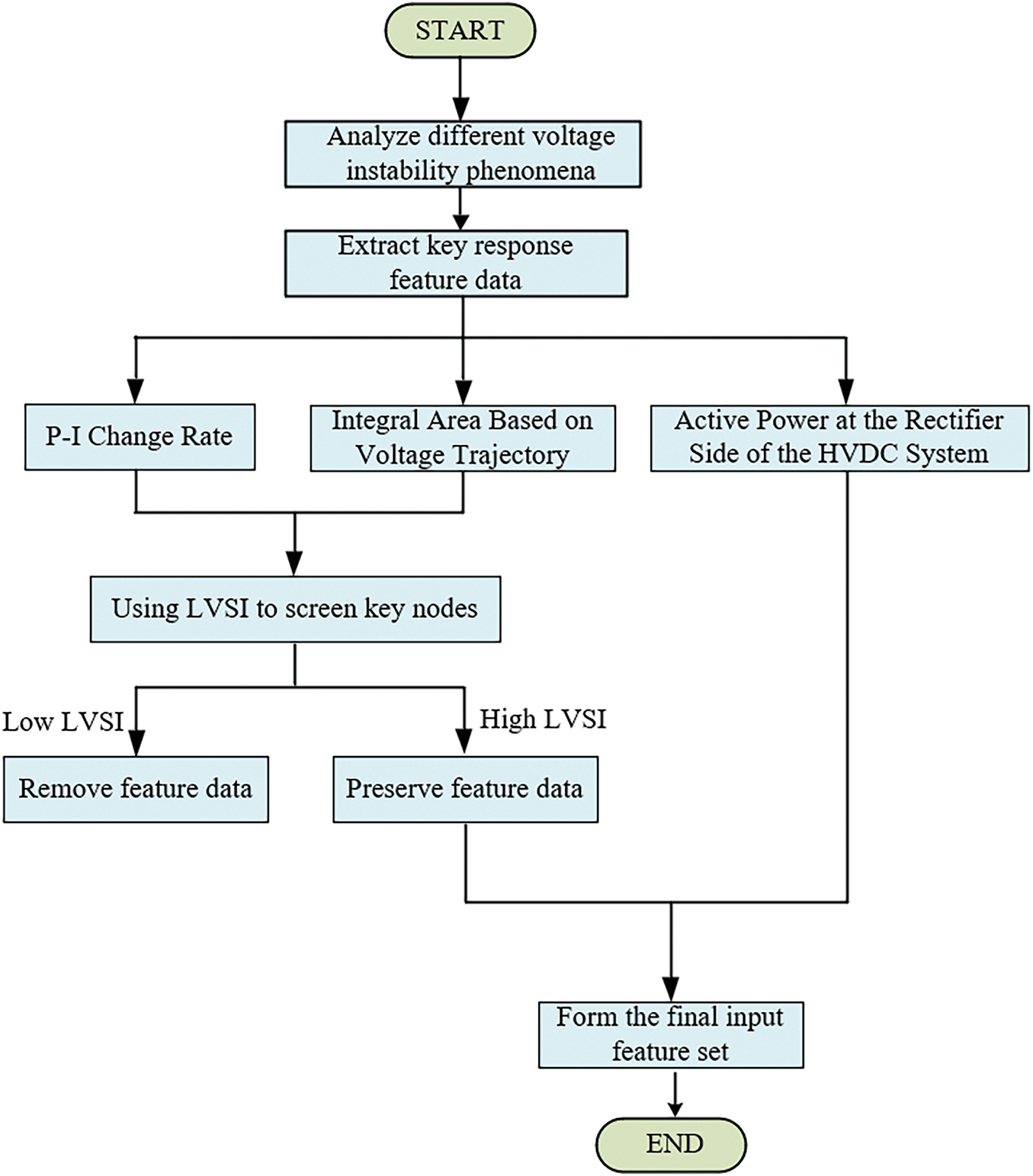
Figure 5: Flowchart of response characteristic data screening framework

3  Composition of Output Set: Transient Voltage Stability Assessment and UVLS Control Strategy

In Section 2, we systematically screened and constructed a set of response characteristics strongly correlated with transient voltage instability, including key physical quantities such as the P-I change rate, the integral area of the voltage trajectory, and the active power at the rectifier side of the DC system. The LVSI index was introduced to focus on critical system nodes, providing a highly interpretable and low-redundancy input foundation for the intelligent response model. Building upon this, Section 3 will further construct an intelligent response framework for transient voltage stability assessment and UVLS control strategy based on these characteristic data, achieving an integrated output from post-fault feature extraction to stability discrimination and control strategy generation.

3.1 Transient Voltage Stability Assessment

To address the issue of transient voltage stability assessment in hybrid AC/DC power systems, an input set is constructed based on the key response characteristic data screened in Section 1. The P-I change rate represents the duration for which a load node remains in the “negative region of increasing current yet losing active power.” The integral area value based on the voltage trajectory reflects different voltage instability states. The duration of active power approaching zero at the rectifier side indicates the severity of power surplus caused by HVDC blocking that cannot be transmitted. Additionally, the node voltage sensitivity index is employed to identify key nodes significantly influencing the system’s transient voltage performance.

The assessment result for each dataset is categorized into two outcomes: An output of 0 indicates transient low-voltage stability, meaning the voltage recovers to above 0.8 p.u. within 10 s after a fault; An output of 1 indicates transient low-voltage instability, referring to either sustained voltage depression or delayed voltage recovery.

The assessment result directly serves as the triggering condition for the UVLS control strategy detailed in Section 3.2. UVLS control is activated when the output is 1.

3.2 UVLS Control Strategy

UVLS is a critical control measure in power systems to prevent voltage collapse [18,19]. When the system experiences a severe disturbance leading to sustained voltage decline, UVLS alleviates system stress by shedding part of the load, thereby restoring voltage to a stable level and preventing voltage collapse or widespread blackouts.

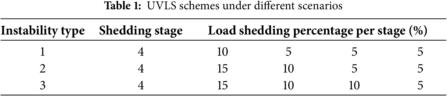
To mitigate transient low-voltage instability, UVLS control strategies are implemented according to the severity of voltage dip trends. Load shedding measures are applied in regions where the load bus voltage fails to recover to above 0.80 p.u. within 10 s after a fault. The trend changes of the three response characteristics reflect, to some extent, the severity of transient voltage instability and characterize the voltage dip trends under different instability scenarios. This, in turn, influences the amount of load shed in each round of UVLS.

As shown in the different voltage recovery trajectories in Fig. 6 and the UVLS load shedding schemes listed in Table 1, varying degrees of voltage dip trends lead to different required amounts of load shedding.

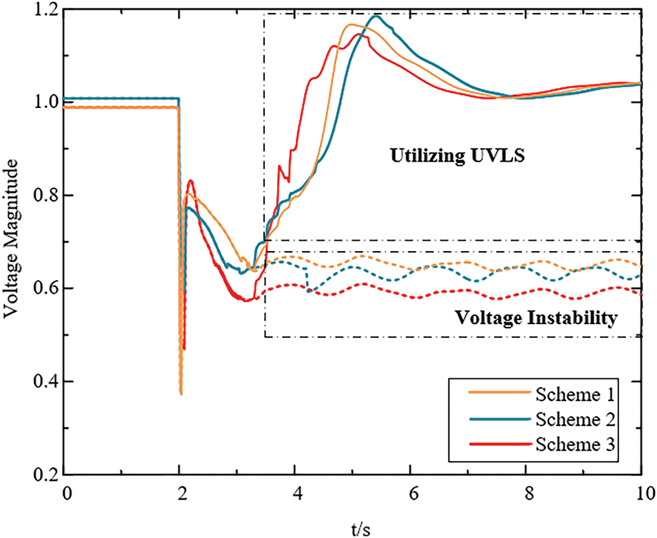
Figure 6: Voltage recovery trajectories under different conditions

In summary, the intelligent response model driven by characteristic response quantities takes the screened response characteristic data as its input, and produces two output components: the first part is the voltage stable/unstable state label, and the second part is the corresponding four-stage UVLS load-shedding amounts for instability scenarios. The input features and output labels are in a one-to-one correspondence, collectively forming the basic structure of the response model. Therefore, the output of the proposed response-driven model in this paper directly determines the decision-making process and execution of the UVLS control strategy. The first output of the model (stable/unstable) serves as the triggering condition for UVLS. When the assessment result is “unstable,” the UVLS control logic is activated; if the result is “stable,” no control action is executed. Once UVLS is triggered, the second output of the model (the load-shedding amounts for the four stages) is used as direct control commands. These output values represent the percentage of load to be shed in each round to restore system stability. This method transforms traditional UVLS into an adaptive intelligent control strategy based on real-time assessment, significantly enhancing the precision and speed of regulation. The overall flowchart is shown in Fig. 7.

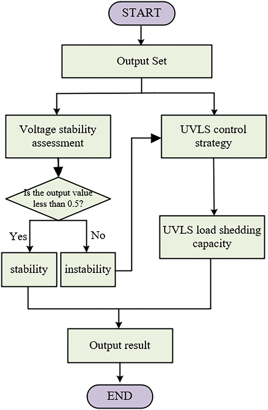
Figure 7: Flowchart of integrated assessment & control intelligent framework

4  The Principle of Hybrid Neural Network and ISAO

In Section 4, the CNN-BiGRU hybrid neural network is used as the core model to achieve the mapping relationship from response features to stable states and control variables. However, the model has a complex structure and numerous hyperparameters, and its performance largely depends on the setting of hyperparameters. Therefore, using ISAO to globally optimize the CNN-BiGRU hyperparameters improves the algorithm’s search efficiency and convergence accuracy, laying the foundation for subsequent model construction and simulation verification.

4.1 CNN-BiGRU Hybrid Neural Network

4.1.1 CNN

As a representative feedforward neural network in deep learning, CNN offers advantages such as processing large-scale data, weight sharing, and capturing spatiotemporal features in sequential data. Typically, CNN consists of an input layer, convolutional layers, pooling layers, fully connected layers, and an output layer [20]. The input layer receives raw data, convolutional layers extract representative feature vectors from the input, pooling layers down sample these features to reduce dimensionality, and the fully connected layer distributes the processed data to regression or classification tasks. Finally, the output layer produces the results, yielding the corresponding output data.

4.1.2 BiGRU

The Gated Recurrent Unit (GRU) neural network uses a reset gate to determine the influence of the previous hidden state on the current hidden state, and an update gate to regulate the extent of this influence. Its structure is simpler than LSTM, and it trains faster [21]. However, GRU processes time series only unidirectionally. In contrast, BiGRU employs two independent GRU layers operating in parallel—one in the forward direction and the other in the reverse direction—and combines their hidden states at each time step, providing more comprehensive temporal feature extraction. Thus, BiGRU can be viewed as a model constructed from two GRUs processing sequences in opposite directions. Its computational formula is given by Eq. (10):

ht=[ht→;ht←]=[GRU(xt,h→t−1),GRU(xt,h←t−1)](10)

where ht→, h→t−1 are the hidden states of the forward GRU at the current and previous time steps, ht←, h←t−1 are the hidden states of the backward GRU at the current and previous time steps, xt is the input at the current time step.

Therefore, the CNN-BiGRU hybrid neural network enables efficient extraction of features from temporal data. By leveraging CNN’s local perception capability through convolutional kernels to mine spatial features in time series, and subsequently introducing BiGRU to capture temporal dependencies, the model effectively addresses regression and prediction tasks.

4.2 ISAO

To improve the prediction accuracy of the model and accelerate the training process, this paper employs the global search capability of ISAO to select the optimal hyperparameter combination for the hybrid neural network, thereby reducing optimization time.

4.2.1 Initialization Phase

The SAO algorithm is a global optimization method inspired by the phenomena of snow sublimation and ablation, which can be applied to optimize hyperparameters of neural networks. SAO primarily consists of two main components: the initialization phase and the exploration-exploitation phase balanced by a dual-population mechanism [22].

First, the SAO algorithm initiates the search with a randomly generated population, analogous to the initial coverage area of snow in nature. Each snow particle (candidate solution) is randomly distributed within this region. Thus, the entire population can be constructed as an n × m matrix A, where n denotes the population size (the number of candidate solutions), and m represents the dimensionality of the solution space (the number of variables in the optimization problem). The expression is as follows:

A=D+λ(U−D)=[a1,1⋯a1,m⋮⋮an,1⋯an,m]n×m(11)

where U and D are the lower and upper bounds of the variable, λ is a random number in [0, 1], ai,j is the value of the j variable corresponding to the i candidate solution.

However, traditional random initialization may lead to uneven population distribution, resulting in local clustering or blank regions, which can reduce global search capability. Therefore, the good point set strategy can be applied during the initialization phase [23]. By leveraging the non-divisibility of prime numbers to avoid periodic overlap, this strategy uniformly fills the space and reduces sampling blind spots. The expression for the good point set is as follows:

r={n⋅pm}(12)

where r is the good point set, pm is the prime number corresponding to dimension m, {·} is the operation of taking the fractional part.

By mapping the good point set rn,m to the initialization phase of SAO, the initial population matrix becomes:

A′=D+r(U−D)(13)

By substituting r for λ in the initialization phase of SAO, the candidate solutions are distributed more uniformly throughout the solution space. This provides a improved foundation for subsequent exploration and exploitation phases, enhancing the overall performance of the algorithm.

4.2.2 Exploration and Exploitation Phase Based on Dual-Population Mechanism Balance

SAO adopts a dual-population mechanism, dividing the population into two subpopulations Pa and Pb. Pa is responsible for the exploration phase, while Pb is used for the exploitation phase.

(1) Exploration Phase

This phase is responsible for conducting a global search within the solution space to prevent the algorithm from prematurely converging to a local optimum. The Pa subpopulation traverses the solution space by simulating the Brownian motion of water vapor molecules [22]. Brownian motion explores potential regions of the solution space through uniform step sizes, as expressed in Eq. (14):

Ax(t+1)=E(t)+BM(t)⊗E→x(t)(14)

where

E→x(t)=β(G(t)−Ax(t))+(1−β)×(∑i=1NAx(t)N−Ax(t))E(t)∈[G(t),A2nd(t),A3rd(t),Ac(t)]Ac(t)=∑i=1NtAx(t)Nt(15)

where Ax(t),Ax(t+1) are the x solutions of the population at time t and t + 1, E(t) is a random variable, BM(t) is a Gaussian distribution based on Brownian motion, E→x(t) is an optimization guiding vector, β is a random number in the interval [0, 1], G(t), A2nd(t), A3rd(t) are the best, second-best, and third-best solutions in the population, Ac(t) is the average of the top 50% solutions by fitness, Nt is a value equal to half the population size.

Although Brownian motion provides certain global search capability, its lack of directional guidance leads to high randomness in later iterations when handling multimodal optimization problems. Therefore, a Gaussian mutation strategy is introduced to adjust the perturbation intensity and direction [22], as expressed in Eq. (16):

GM(t)=σ(t)⋅N(0,σD2)=σ0⋅e−γ⋅tDtMAX⋅N(0,σD2)(16)

where GM(t) is the Gaussian mutation vector, σ(t) is the standard deviation that varies with iterations, N(0,σD2) is a multidimensional standard normal distribution, σ0 is the initial standard deviation, γ is the decay coefficient (typically set to 2), tD is the current iteration number, tMAX is the maximum number of iterations.

The Gaussian mutation strategy is combined with the position update in the exploration phase of SAO as follows:

Ax(t+1)=E(t)+(BM(t)+GM(t))⊗E→x(t)(17)

By integrating the Gaussian mutation strategy with Brownian motion, the randomness of Brownian motion helps maintain population diversity, while the Gaussian mutation strategy expands the search range for optimal solutions. Additionally, an exponential decay mechanism gradually reduces perturbation intensity over time, enhancing the algorithm’s global optimization capability and local exploitation efficiency.

(2) Exploitation Phase

This phase focuses on fine-grained search within known preferred regions of the solution space. The Pb subpopulation traverses the solution space by simulating the process of snow melting into liquid water, primarily using the degree-day method to exploit around the current best solution. The formula is:

Ax(t+1)=qG(t)+BM(t)⊗F→x(t)(18)

where

F→x(t)=β1(G(t)−Ax(t))+(1−β1)×(∑i=1NAx(t)N−Ax(t))q=ADDF×(T¯−Tl)ADDF=θ1+θ2⋅etDtMAX−1(e−1)(19)

where q is the snow ablation rate, F→x(t) is a guiding vector, β1 is a random number in [−1, 1], ADDF is the snow ablation coefficient, T¯ is the average daily temperature, T1 is the base temperature, θ1,θ2 are constants.

In summary, the good point set strategy is applied in the initialization phase of SAO to ensure uniform distribution of initial solutions across a broader solution space. In the exploration phase, the Gaussian mutation strategy is integrated with Brownian motion, and an adaptive standard deviation dynamically adjusts perturbation intensity, improving convergence speed and solution accuracy.

4.3 ISAO-CNN-BiGRU

For the CNN-BiGRU model, its ultimate performance depends on the selection of hyperparameters. These hyperparameters collectively determine the model’s training capability and generalization performance. This paper primarily utilizes ISAO to optimize the following five hyperparameters:

1) Learning rate: Controls the step size of gradient updates in the optimization algorithm;

2) Number of CNN convolutional kernels: Determines the quantity of spatiotemporal feature maps that the convolutional layer can extract, directly influencing the model’s ability to capture local features in the input data;

3) Number of BiGRU neurons: Governs the model’s capacity to model long-term dependencies in time series;

4) Dropout rate: Serves as an effective means to control model complexity and prevent overfitting;

5) Batch size: Affects the stability of the training process and the generalization performance of the model.

The process of optimizing CNN-BiGRU hyperparameters with ISAO can be regarded as a high-dmensional black-box optimization problem. The core objective is to find an optimal set of hyperparameters J through the ISAO algorithm to minimize the loss function of the CNN-BiGRU model on the validation set. This can be expressed as:

J∗=arg⁡minJL(J)(20)

where J={V,NCNN,NGRU,PDropout,B}, V is learning rate, NCNN is number of CNN convolutional kernels, NGRU is number of BiGRU neurons, PDropout is dropout rate, B is batch size.

When using ISAO to perform hyperparameter optimization for CNN-BiGRU, the initialization of ISAO is first carried out according to Eq. (13). The good point set strategy is employed to generate the initial population, replacing traditional random initialization and ensuring a uniform distribution of candidate solutions in the solution space. This effectively avoids the issues of population clustering or blank areas that may arise from traditional random initialization, laying a solid foundation for subsequent global search. Each snow particle position in ISAO represents a candidate solution J. At each iteration l, the ISAO population P is divided into Pa and Pb for exploration and exploitation.

Individuals in subpopulation Pa perform global exploration based on Brownian motion and Gaussian mutation. This can be expressed as:

Jit+1=Jit+η⋅Bt+Mt(21)

where η is the step size, Bt is the Gaussian mutation vector, Mt is a Gaussian distribution based on Brownian motion.

This strategy enhances global exploration capability in the early iterations and gradually shifts to local fine-tuning in later stages, effectively balancing exploration and exploitation.

Individuals in subpopulation Pb perform local refinement around the current best solution. This can be expressed as:

Jit+1=Jit+γ⋅(Jbestt−Jit)(22)

where γ is the exploitation step size, and Jbestt is the historical best solution found by generation l.

Therefore, for each candidate solution J in the population, the optimal solution (the optimal parameter combination) is obtained through the following steps:

1) Initialize the hyperparameter population using the good point set strategy and configure the hyperparameter combinations into the CNN-BiGRU model;

2) Train each candidate solution and compute the loss function on the test set. To more intuitively represent the optimal combination, the coefficient of determination R² is used as the output objective function;

3) Update the population based on the value of the coefficient of determination, performing searches in the exploration and exploitation phases respectively;

4) Iterate until the maximum number of iterations is reached;

5) Output the optimal hyperparameter combination.

The final output of this optimization process is the globally optimal hyperparameter combination Jbest that enables the CNN-BiGRU model to achieve the best performance on the test set.

5  Construction of CNN-BiGRU Model Driven by Response Characteristic Data and Optimized with ISAO

To achieve accurate assessment of transient voltage stability in hybrid AC/DC power systems and propose corresponding control strategies, a CNN-BiGRU model driven by response characteristic data and optimized with ISAO is constructed. The core of this model lies in utilizing response characteristic data to build the input training set, integrating the advantages of CNN and BiGRU, and optimizing key hyperparameters of the neural network through ISAO to obtain the output results.

By constructing response characteristic data that reflect the system’s transient behavior, a training set for driving the response model is formed. Subsequently, the combination of CNN and BiGRU enables the neural network to deeply extract information about the system’s transient behavior embedded in the response characteristic data generated based on physical mechanisms. However, given the complex structure of the CNN-BiGRU hybrid model and its sensitivity to hyperparameter settings, relying solely on its inherent search mechanism is not only inefficient but also prone to local optima. Therefore, the SAO algorithm, enhanced with a good point set initialization strategy and a Gaussian mutation strategy, is employed to globally optimize the key hyperparameters of this hybrid neural network. The powerful global search and local exploitation capabilities of ISAO efficiently identify the optimal hyperparameter combination, maximizing the model’s accuracy and generalization ability while accelerating the training convergence process. The structure of the comprehensive model constructed in this chapter is illustrated in Fig. 8.

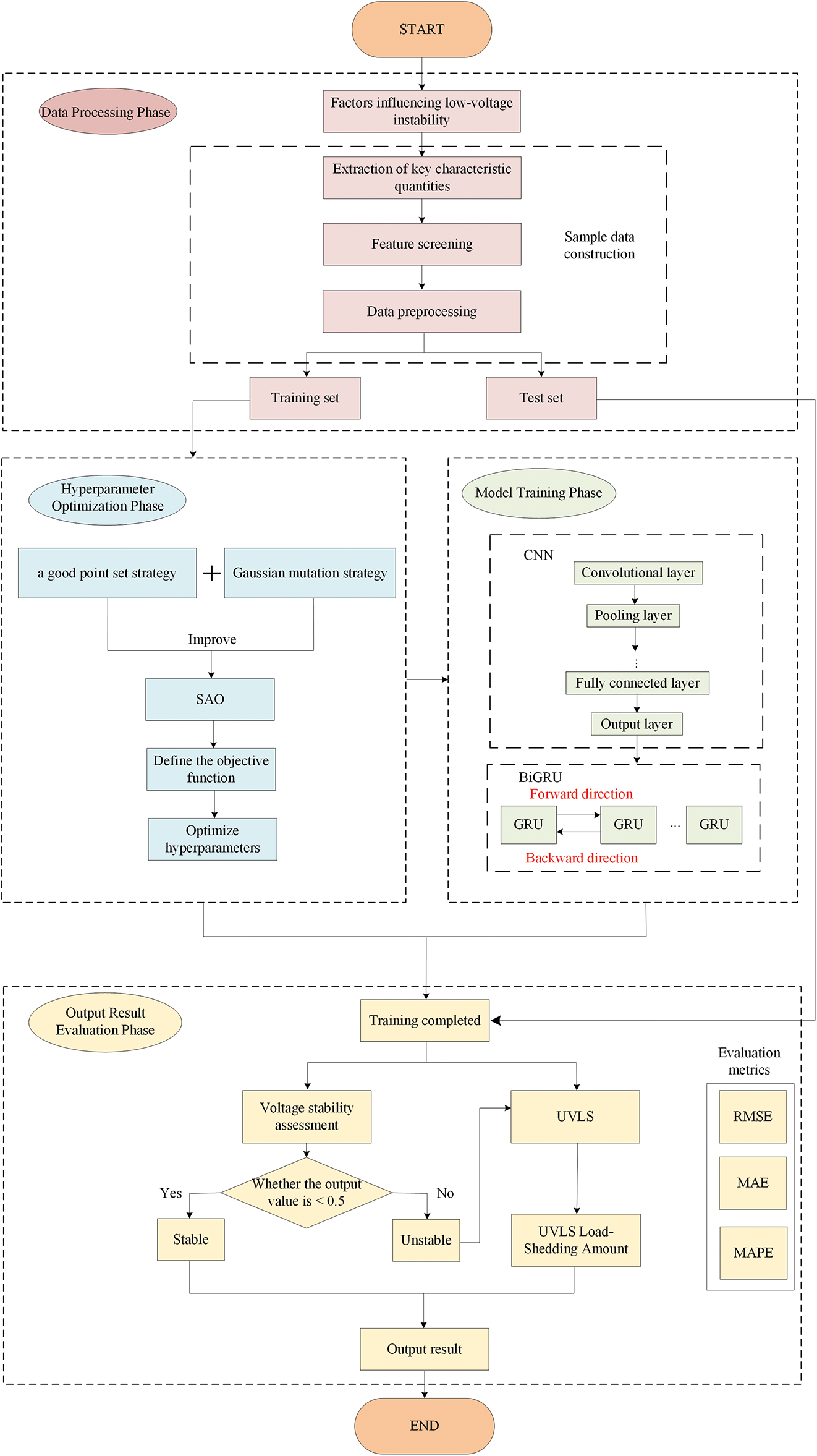
Figure 8: Process of model construction

The specific steps are as follows:

(1) Data Processing Phase: Extract response characteristic data from transient low-voltage instability scenarios in hybrid AC/DC power systems. Quantify the correlation between load bus voltage fluctuations and LVSI, screen key regions significantly influencing transient stability, and preprocess the characteristic data to determine the training and prediction sets for the neural network.

(2) Hyperparameter Optimization Phase: Use the output result error as the objective function and apply the ISAO algorithm to optimize the hyperparameters of the hybrid neural network.

(3) Model Training Phase: Construct the CNN-BiGRU hybrid neural network architecture. Use the screened feature set as input and the voltage stability state along with the load-shedding amount of the UVLS control strategy as output labels. Train the model on the input response characteristic data.

(4) Output Result Evaluation Phase: Quantify model performance using Root Mean Squared Error (RMSE), Mean Absolute Percentage Error (MAPE), Mean Absolute Error (MAE), and Coefficient of Determination (R²). Simultaneously validate the dual-task output. Compare the results with other neural networks to demonstrate the superiority of the proposed method in transient stability discrimination accuracy and load-shedding strategy effectiveness.

5.1 Data Processing Phase

Neural networks typically consist of three parts: an input layer, hidden layer, and an output layer. Firstly, the input layer receives training data. Then, the hidden layer process the received data using neurons, hyperparameters, and activation functions. Finally, the output layer generates the corresponding results. When using neural networks for transient voltage assessment and control, the input layer often includes various electrical quantities related to the faulted bus voltage, but these lack clear physical interpretability. Therefore, typical characteristic quantities representing transient low-voltage instability can be extracted as input data for the training set, while the voltage stability/instability status and the corresponding load-shedding amounts of control strategies serve as output labels. However, since the input features have different dimensions, directly fitting them into the model would introduce accuracy deviations. Thus, normalization is applied to address the issue of inconsistent input data dimensions [24]:

Z=z−zminzmax−zmin(23)

where Z is the normalized input data, z is the raw data, zmax and zmin are the maximum and minimum values of z.

5.2 Hyperparameter Optimization Phase

Firstly, set the population size of the ISAO to 8 and the maximum number of iterations to 30, and define the lower and upper bounds for five hyperparameters. Additionally, establish an elite pool containing four elite individuals, which includes the current global best solution, the second-best solution, the third-best solution, and the mean of the top 50% best individuals. This strategy effectively leverages historical optimal information to guide the population evolution and accelerate the convergence process.

Traditional methods for selecting neural network hyperparameters typically rely on trial-and-error, which is time-consuming and offers no guarantee of prediction accuracy. Therefore, this paper employs the ISAO optimization method to optimize the hyperparameters of the hybrid neural network. The specific steps are shown in Fig. 9.

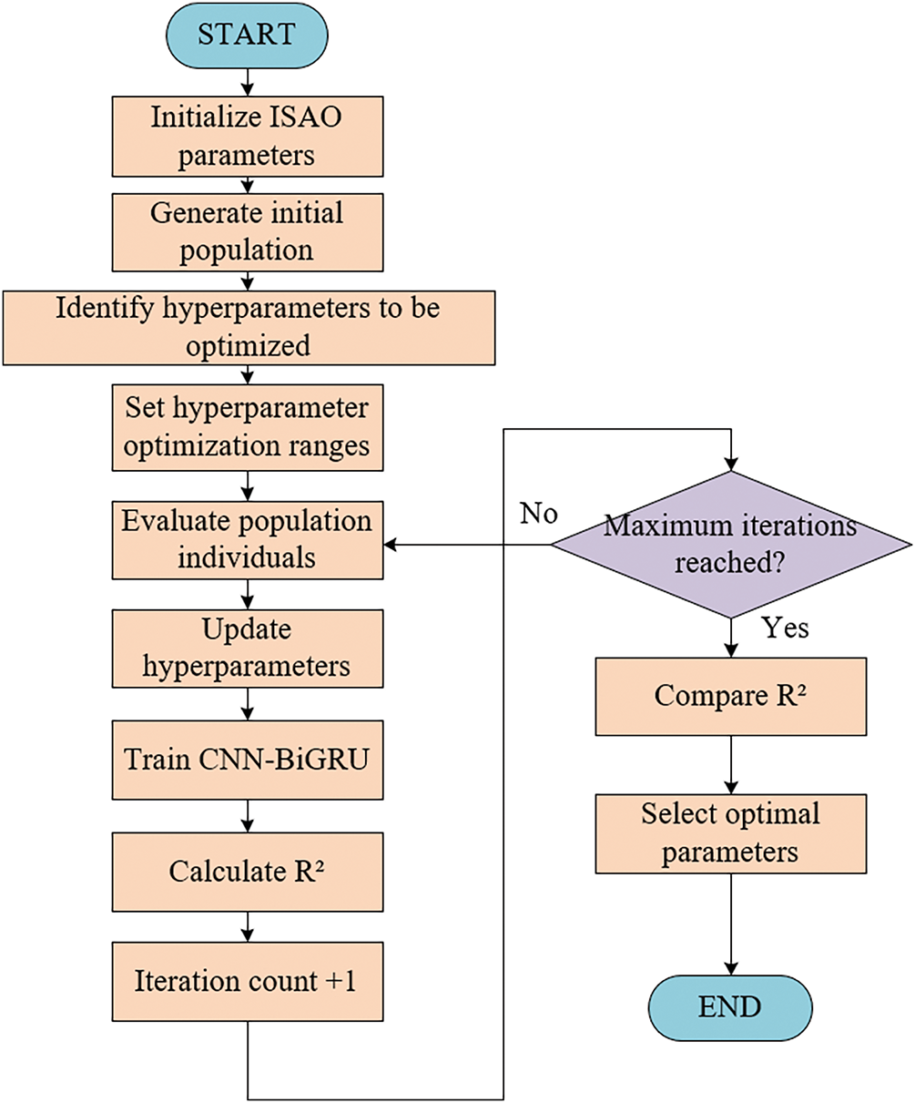
Figure 9: Flowchart of ISAO hyperparameter optimization

Step 1: Initialize ISAO parameters, generate the initial population, determine the hyperparameters to be optimized, and set the hyperparameter search ranges.

Step 2: Evaluate a set of population individuals in the ISAO algorithm, update the corresponding hyperparameters, train the hybrid neural network model, and obtain the coefficient of determination value of the model.

Step 3: After each output of the coefficient of determination, check whether the maximum number of iterations has been reached. If not, continue selecting optimized parameters; if reached, compare the coefficient of determination values of all sets and choose the optimal parameters.

Step 4: Output the optimized parameters, concluding the optimization process.

5.3 Model Training Phase

Key features are determined through feature screening, and corresponding hyperparameters are selected during the hyperparameter optimization phase to construct a spatiotemporally fused input data structure. The network architecture adopts a collaborative mechanism of CNN and BiGRU. The CNN module uses a 2D CNN architecture with three convolutional layers and one pooling layer, activated by the ReLU function. The convolutional layers have a kernel size of 3 × 3, a stride of 1, and “Same” padding. The number of kernels is automatically selected after hyperparameter optimization. The pooling layer uses a 3 × 3 kernel, a stride of 1, and “Valid” padding. The CNN output is reshaped into sequences and fed into the BiGRU temporal modeling layer. The number of neurons in its bidirectional structure is also automatically optimized via ISAO. The training process adopts a dynamic optimization strategy, and the Dropout rate is optimized through ISAO to suppress overfitting. Finally, generate the corresponding results through the output layer.

5.4 Output Result Evaluation Phase

To evaluate the model’s accuracy, this paper selects the RMSE, MAE, MAPE and R² as evaluation metrics, establishing an output result evaluation system. The expressions are as follows:

RMSE=1h∑i=1h(yi−y^i)2(24)

MAE=1h∑i=1h|yi−y^i|(25)

MAPE=1h∑i=1h|yi−y^i|yi(26)

R2=∑i=1h(y^i−1h∑i=1hyi)2∑i=1h(yi−1h∑i=1hyi)2(27)

where: h is the number of predicted data points, y^i is the predicted value, yi is the actual value.

The model’s accuracy is higher when the results of Eqs. (24)–(26) are smaller and the result of Eq. (27) is closer to 100%.

6  Simulation Analysis

6.1 Simulation Case Study

To validate the effectiveness of the proposed method, an improved CEPRI 36-node simulation model was developed on the PSASP simulation platform. In this model, the original synchronous generator at Bus 3 was replaced by a wind farm consisting of doubly-fed induction generators, which is connected to the AC system via two HVDC transmission lines. The renewable energy penetration in this system accounts for 20%. The system operates at a rated frequency of 50 Hz and a base power of 100 MVA. The topology is shown in Fig. 10.

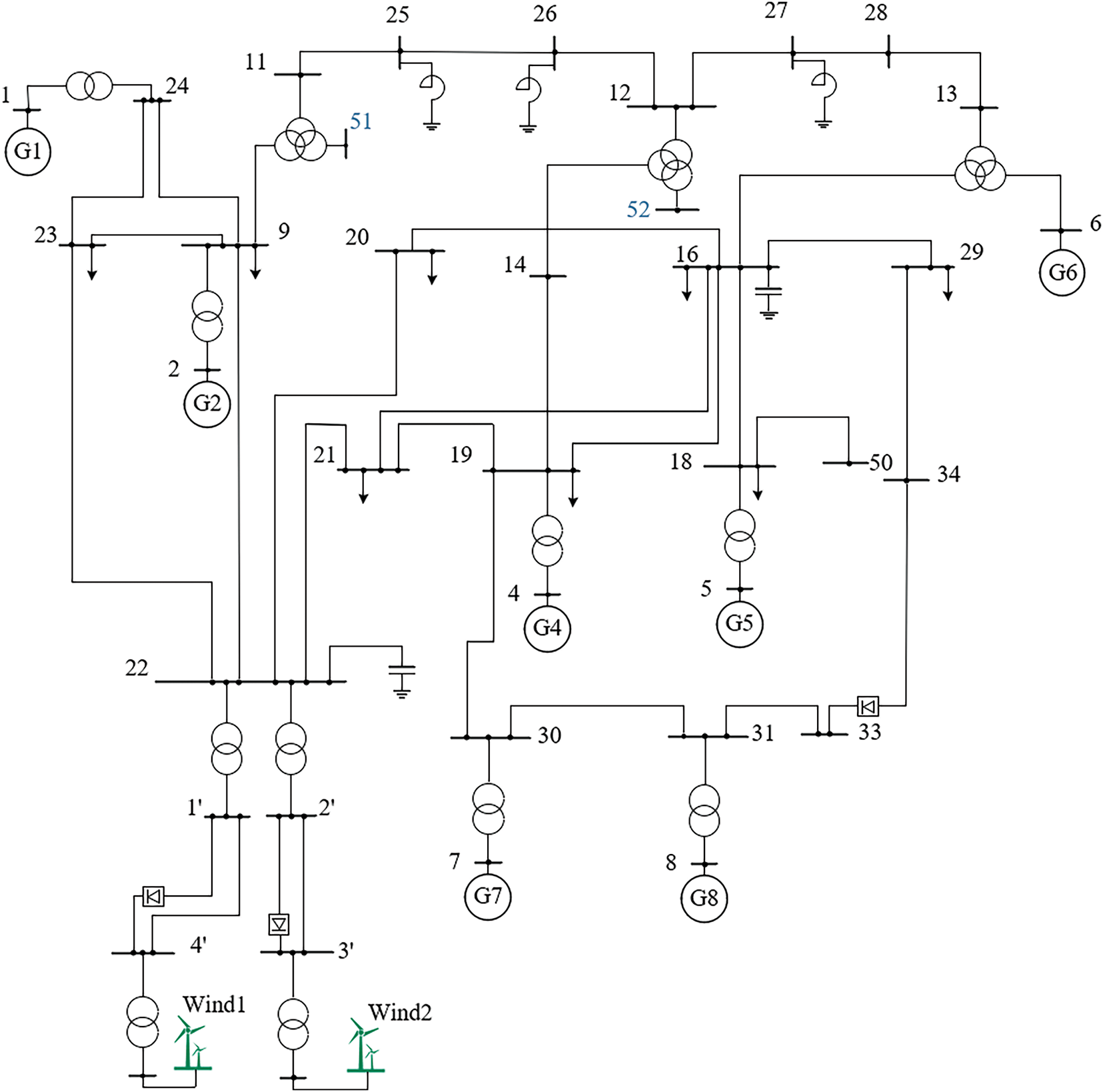
Figure 10: Topology of the improved CEPRI 36-node system

Considering the load fluctuations and the stochastic nature of renewable energy output, the sample set was constructed based on variations in load and renewable energy generation. On the basis of 90% to 110% of the baseline load, the load was increased in 2% increments, while the output power of generators was proportionally adjusted accordingly. Each change in load and generator output was treated as a distinct power flow calculation scenario. The specific fault settings were as follows:

1) Three-phase short-circuit fault criteria were established for each transmission line, analyzing influencing factors such as faults at different system buses and varying fault durations;

2) For scenarios with DC grid integration, the predefined faults included system transient voltage stability analysis under conditions where any DC line experiences blocking or commutation failure.

Secondly, the product of the active power and current value of the load within 0.2 s after fault clearance, along with the active power at the rectifier side of the HVDC system, are selected. Additionally, the integral area of the voltage trajectory at the oscillation center and its adjacent critical nodes after the fault is calculated. These values are used as characteristic data. A total of 4000 sample datasets are generated, comprising 1554 stable cases and 2446 unstable cases.

Finally, the average LVSI value for each load node (or bus) after fault clearance is computed. Feature data associated with load nodes (or buses) exhibiting higher LVSI values are selected as the training set for the neural network, while those with lower LVSI values are discarded. The top four load nodes with the highest LVSI values under each fault scenario are statistically identified, as illustrated in Fig. 11.

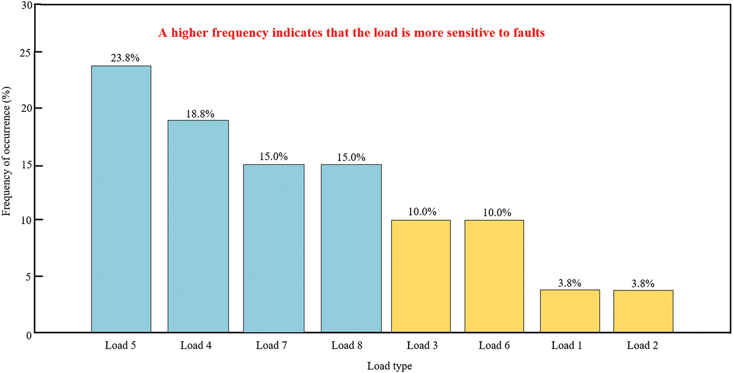
Figure 11: Statistical results of LVSI

Among them, Load 4, Load 5, Load 7, and Load 8 exhibit a higher frequency of high sensitivity values. Therefore, the characteristic quantities of these four loads were selected for further analysis. After feature screening, the 4000 datasets were divided into two parts: 70% were selected as the training set, and the remaining 30% were used as the test set for result prediction.

Next, R² of the CNN-BiGRU model was used as the objective function of the optimization algorithm to optimize the learning rate, the number of CNN convolutional kernels, and the number of neurons in the hidden layers of BiGRU. For comparison, the unimproved SAO algorithm, the Bayesian Optimization (BO) algorithm and the Triangulation Topology Aggregation Optimizer (TTAO) algorithm were also applied to optimize the same neural network [25]. The results are shown in Table 2.

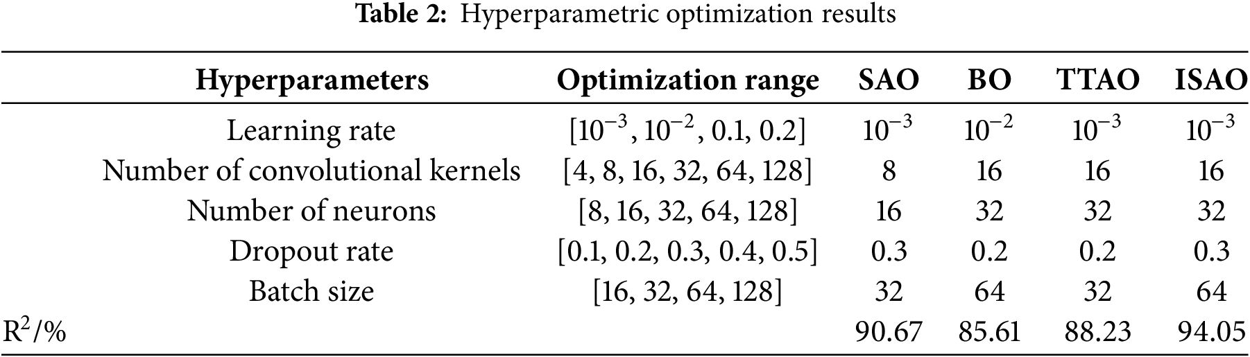
According to Table 2, after hyperparameter optimization using the ISAO algorithm, R² of CNN-BiGRU reaches 94.05%, demonstrating the high efficiency of the proposed optimization method.

Finally, the optimized neural network was used to train the characteristic data. Since no control strategy is required when the voltage is stable, the first output label was used as the benchmark for voltage stability assessment. If the evaluated value is less than 0.5, the voltage is considered stable; otherwise, it is considered unstable. For the latter case, the corresponding UVLS control strategy is proposed based on the load-shedding amount from the second part of the output.

Fig. 12 shows the evaluation results of the first output label, with an accuracy rate of 97.50%. Therefore, when the voltage stability assessment result is less than 0.5, it can be directly output as a stable voltage state without invoking the UVLS control strategy based on the second output label.

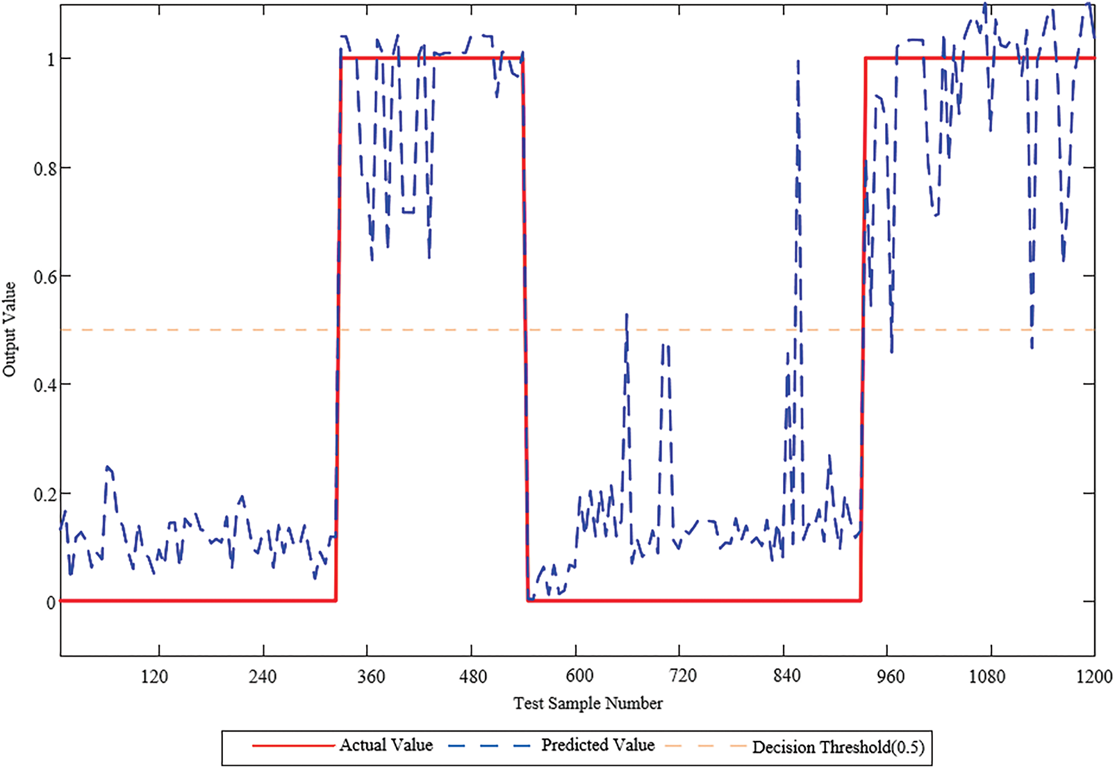
Figure 12: Assessment result of voltage stability/instability

To further verify the reliability of the data, we shuffled the test set and introduced k-fold cross-validation, specifically 5-fold cross-validation, to reassess the model’s performance. This ensures that the model is trained and tested on multiple different data subsets, providing a more robust and reliable performance evaluation. The evaluation results, also presented in Fig. 13, show a model accuracy of 97.25%.

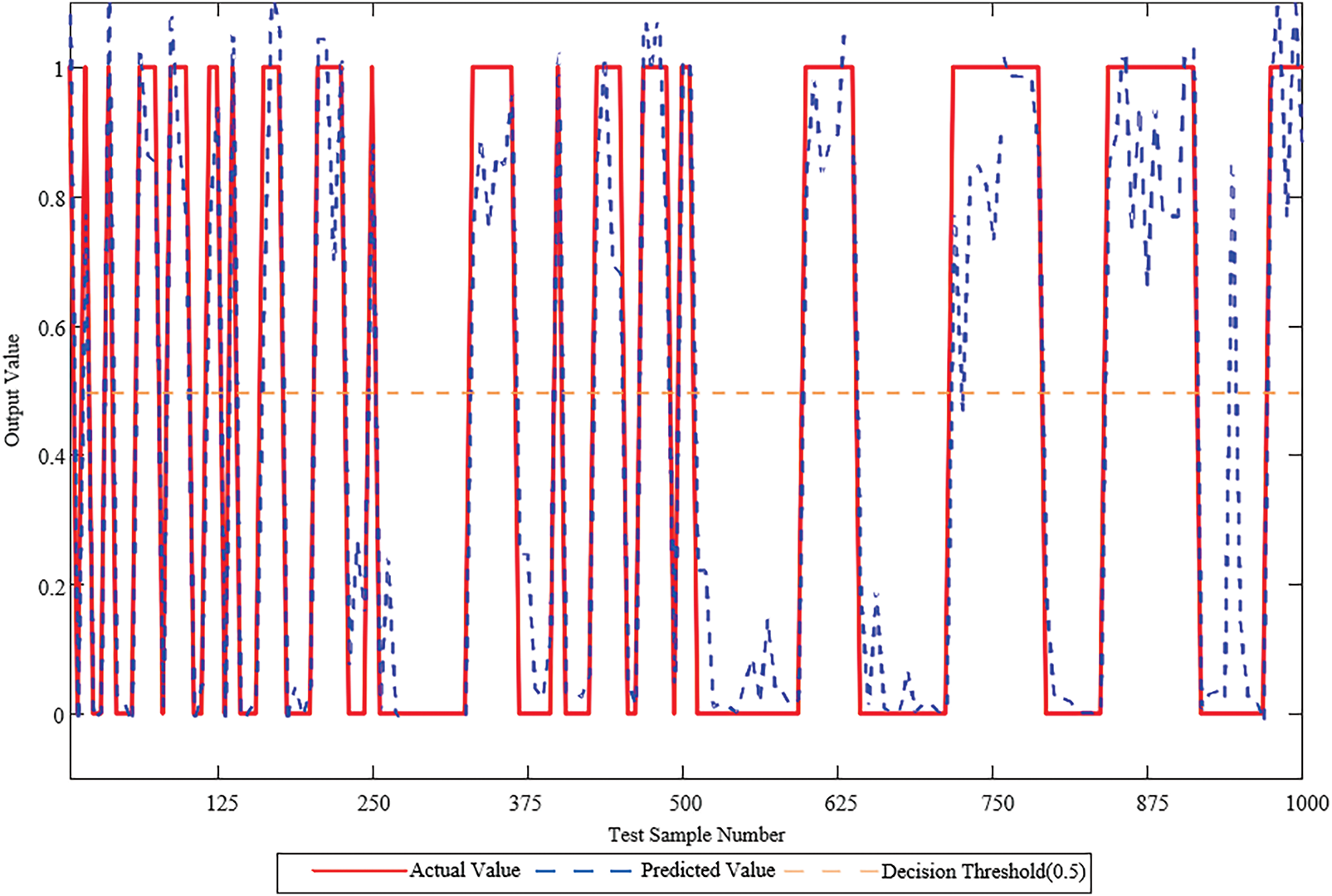
Figure 13: Assessment result of voltage stability/instability under k-fold cross-validation

For the results of the second output, seven different methods were selected for model accuracy comparison: LSTM, CNN-LSTM, CNN-BiGRU, SAO-CNN-BiGRU, BO-CNN-BiGRU, TTAO-CNN-BiGRU and the proposed method. As shown in Fig. 14, CNN-BiGRU demonstrates higher accuracy compared to other neural networks. Furthermore, the ISAO-CNN-BiGRU model exhibits better fitting performance than both TTAO-optimized and SAO-optimized versions, with results closer to the actual values and significantly smaller fluctuations compared to other methods.

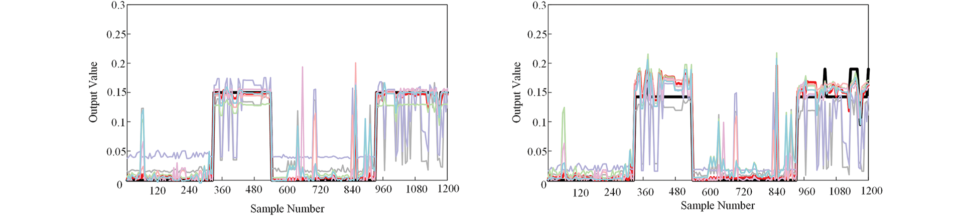
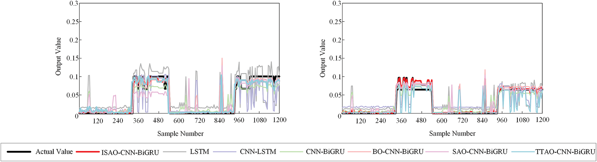
Figure 14: Output results of different methods

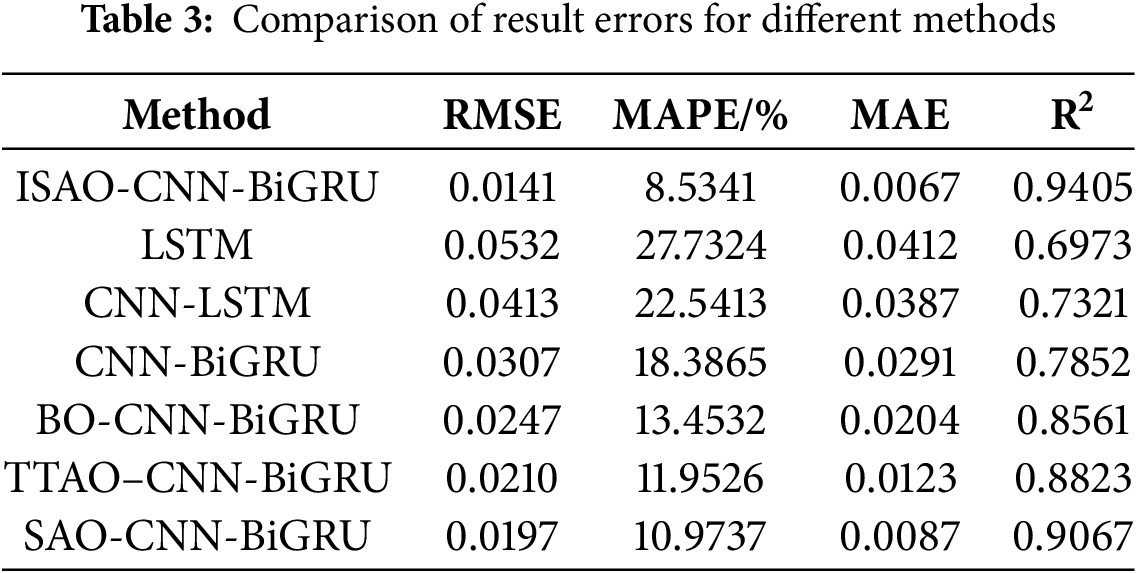
To more intuitively reflect the accuracy of the neural network, an error analysis was conducted using four evaluation metrics: RMSE, MAE, MAPE, and R². The results are shown in Table 3. It can be observed that the proposed ISAO-CNN-BiGRU model exhibits smaller errors compared to LSTM and CNN-LSTM. Furthermore, the CNN-BiGRU model optimized with ISAO achieves R² closer to 1.

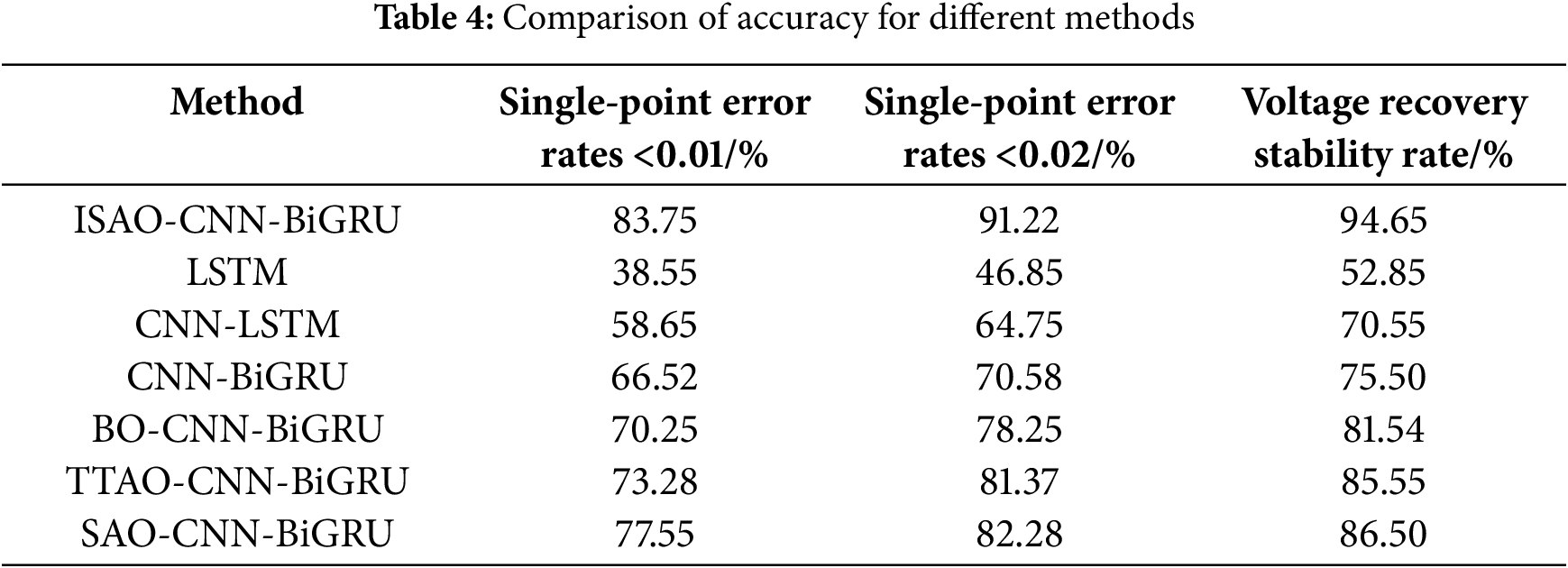
To further validate the accuracy of the UVLS load-shedding amounts from the second output, the single-point error rates (within ±0.01 and ±0.02 ranges) for the predicted values of the four output labels and the voltage recovery stability rate achieved by the UVLS control strategy were compared across the seven aforementioned methods under voltage instability conditions. The results in Table 4 demonstrate that the proposed method significantly outperforms others in both single-point error control and voltage recovery stability rate, proving that the neural network model based on response characteristic data can rapidly generate accurate control decisions and effectively restore system voltage stability.

Additionally, the system’s operation under a three-phase short-circuit fault condition was selected for testing. A three-phase short-circuit fault was applied to line 12–26 at 2 s and cleared at 2.1 s. The system voltage waveform is shown in Fig. 15a. After being disturbed, the voltage magnitude dropped, causing it to temporarily fail to recover above the 0.8 p.u. threshold, thus requiring voltage control measures.

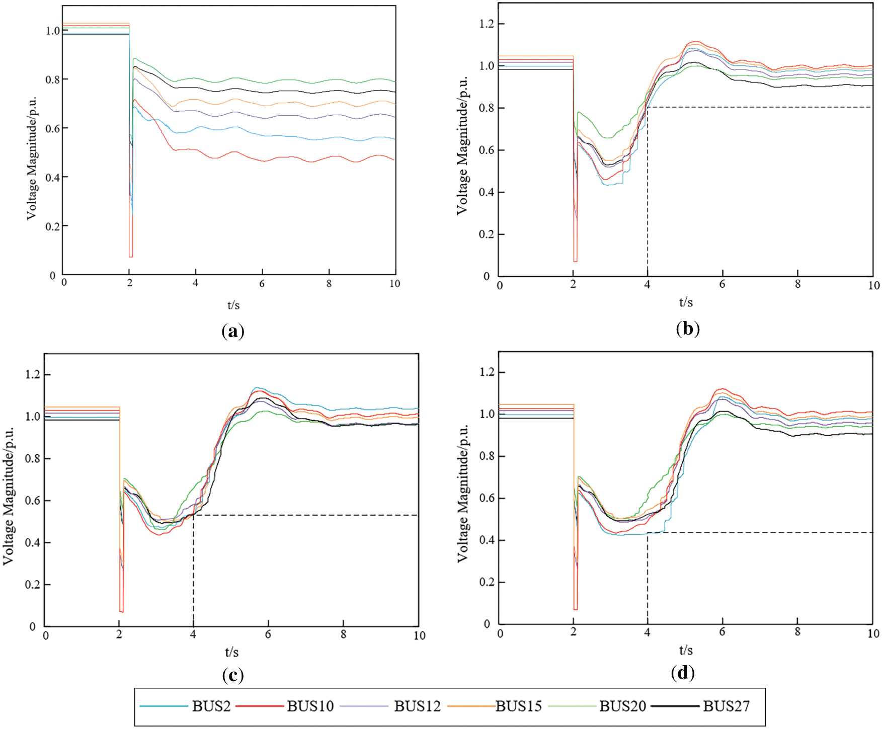
Figure 15: Voltage values regulated by different methods. (a) Bus voltages before control; (b) Bus voltages after control by the proposed method; (c) Bus voltages after control by traditional UVLS; (d) Bus voltages after control by traditional compensation measures

The proposed method was applied for regulation, and the voltage waveform after execution is shown in Fig. 15b. Compared with the effect of traditional UVLS shown in Fig. 15c, the proposed method enables rapid recovery above 0.8 p.u. after the fault. Furthermore, a comparison was made with the voltage regulation effect of traditional reactive power compensation, as shown in Fig. 15d. The results demonstrate that the proposed method can ensure faster and more accurate voltage recovery compared to traditional approaches.

Therefore, the proposed control method exhibits strong adaptability in this scenario, enabling rapid and accurate support for system voltage recovery.

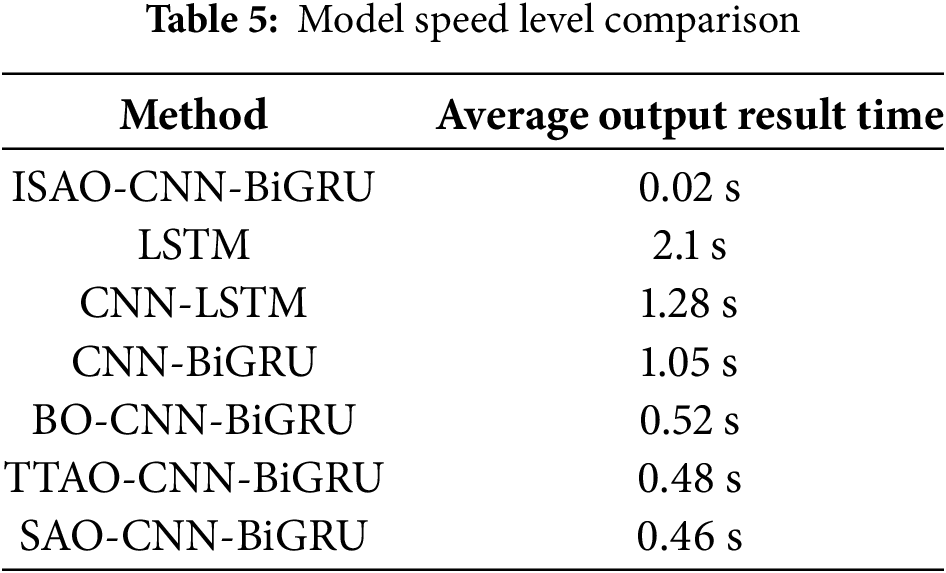
The average output result times of multiple models were compared simultaneously, as shown in Table 5. Model evaluation time refers to the computational time required for a trained model to complete one forward propagation and produce an output when processing a single input sample. This metric serves as a core performance indicator for measuring whether an intelligent response framework can meet the requirements of real-time control. It can be observed that the proposed ISAO-CNN-BiGRU model achieves the shortest output time compared to other methods. Therefore, it can be demonstrated that the proposed response-driven model not only achieves higher accuracy but also exhibits excellent timeliness.

To comprehensively evaluate the applicability of the proposed ISAO-CNN-BiGRU model, its robustness against noise interference was validated. Gaussian white noise of varying intensities was superimposed onto the characteristic data of the test set to simulate measurement errors and disturbance uncertainties in practical power systems. This tested the model’s generalization capability and robustness under non-ideal data conditions. The results are shown in Fig. 16.

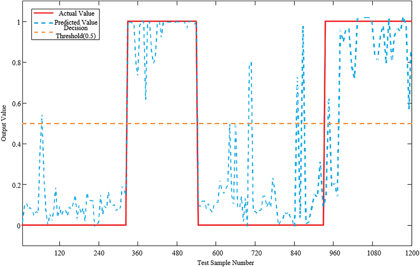
Figure 16: Assessment result of voltage stability/instability after adding noise

When the same Gaussian white noise is added, the error comparison of the UVLS load-shedding amounts between the proposed method and other methods is shown in Table 6.

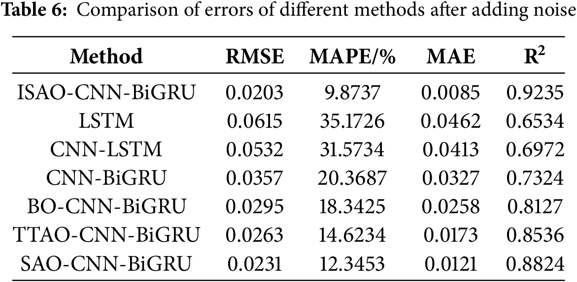
It can be observed that after adding Gaussian white noise, although the accuracy slightly decreases compared to the noise-free condition, the proposed method still maintains significant advantages over other approaches. This fully demonstrates the strong robustness of the response model against data noise and its reliable assessment and decision-making capabilities in complex environments.

6.2 Actual Case Study

To validate the feasibility and superiority of the proposed method in practical power grid applications, tests were conducted using actual data from a 500 kV main grid of a regional hybrid AC/DC interconnected power system in China. The topology is shown in Fig. 17. The installed capacity ratio of renewable energy to conventional power sources is 1:2.62, with renewable energy generating 1800 MW and HVDC receiving power of 800 MW.

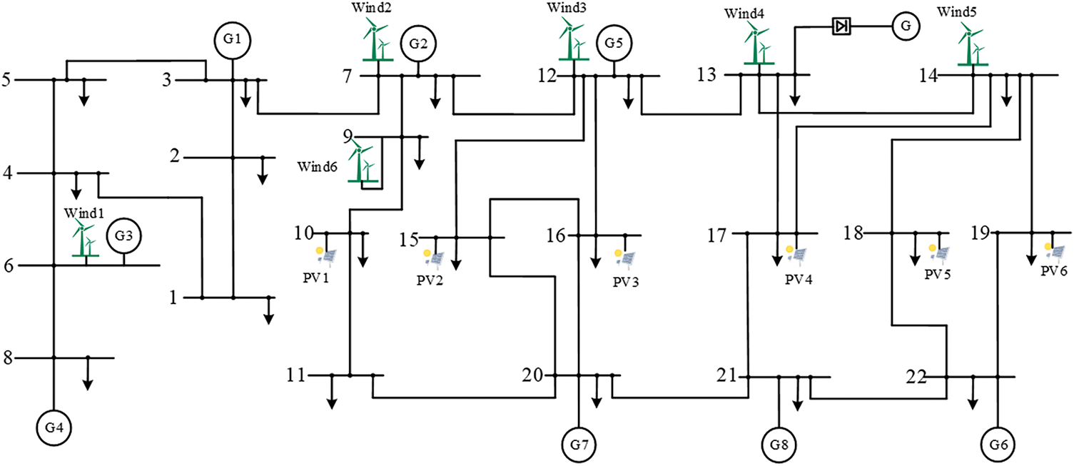
Figure 17: Topology of actual power grid

Characteristic data under different faults were selected as input for model training, generating a total of 3500 sample datasets, including 1400 stable cases and 2100 unstable cases. After feature screening, the 3500 datasets were divided into two parts: 70% were used as the training set, and the remaining 30% were used as the test set for result prediction.

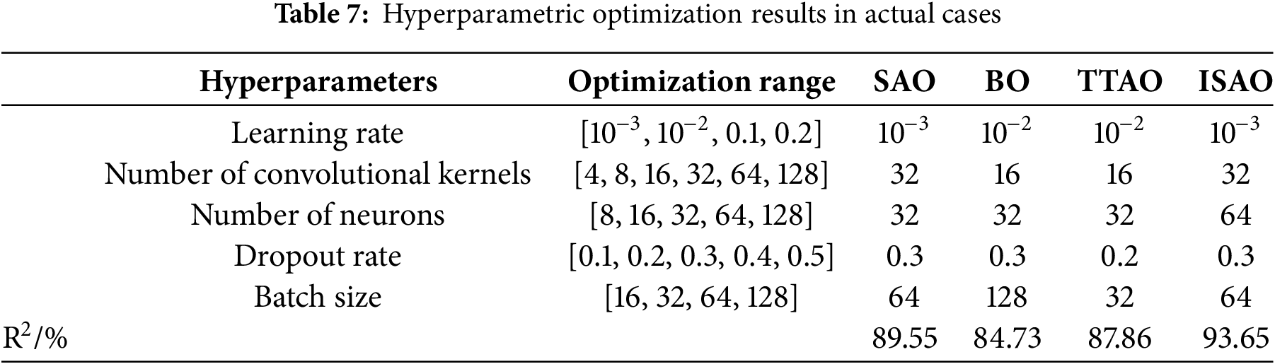
When training and testing with the sample set from the actual power grid data, the results of hyperparameter optimization using ISAO changed compared to the standard simulation case due to the increased number of selected nodes. The results are shown in Table 7.

To verify the effectiveness of the test set, the test set was shuffled and compared for validation. Fig. 18 shows the evaluation result of the first output label, with an accuracy of 97.60%. Therefore, when the voltage stability evaluation result is less than 0.5, it is directly output as a stable voltage state.

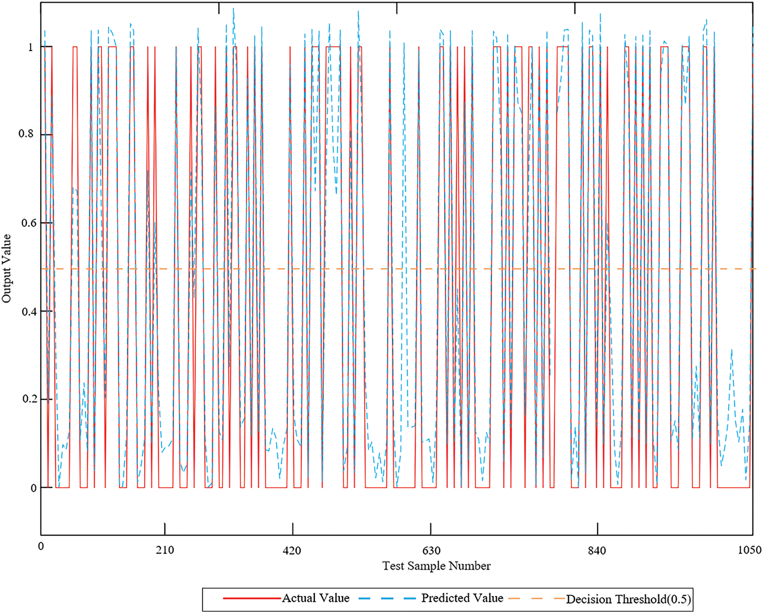
Figure 18: Comparison of evaluation metrics for different methods in actual cases

Using the optimized hyperparameters, the proposed model was trained. For the results of the second output, seven different methods were again selected for model accuracy comparison. An error analysis was conducted using four evaluation metrics—RMSE, MAE, MAPE, and R²—with the results shown in Fig. 19. Compared to the other methods, the proposed method achieves significantly lower values in RMSE, MAE, and MAPE, while its coefficient of determination R² is closest to 1.

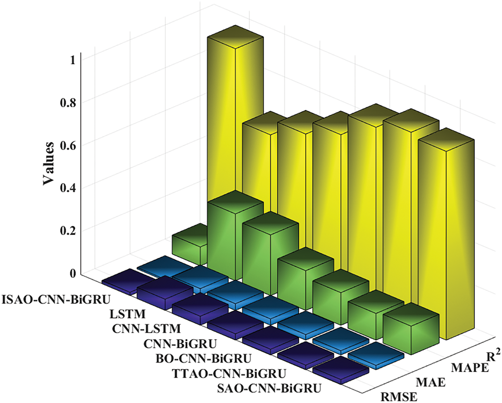
Figure 19: Comparison of evaluation metrics for different methods in actual cases

Additionally, the system’s operation under a three-phase short-circuit fault condition was tested. A three-phase short-circuit fault was applied on the AC1 side, initiated at 2 s and cleared at 2.09 s. The system voltage waveform is shown in Fig. 20a. When the proposed method was implemented for regulation, the resulting voltage waveform after execution is presented in Fig. 20b. Comparisons were made with the conventional UVLS method shown in Fig. 20c and the traditional reactive power compensation-based voltage regulation method depicted in Fig. 20d. The results demonstrate that the proposed method enables faster and more accurate voltage recovery compared to conventional approaches.

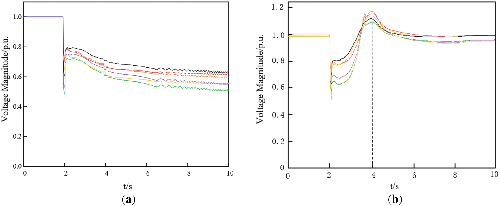
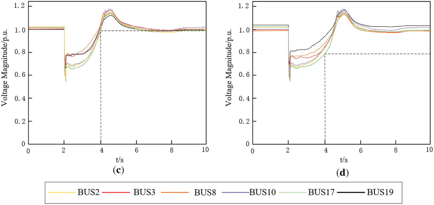
Figure 20: Voltage values adjusted through different methods in actual cases. (a) Bus voltages before control; (b) Bus voltages after control by the proposed method; (c) Bus voltages after control by traditional UVLS; (d) Bus voltages after control by traditional compensation measures

To evaluate the model’s robustness against disturbances, missing data tests and communication delay simulation tests were conducted. The missing data tests were designed to assess the model’s tolerance to incomplete data, while the delay simulation tests introduced delay steps between internal time steps of the samples to evaluate its adaptability to data acquisition delays. The RMSE values under disturbance-free conditions were compared with those obtained during the tests to determine accuracy, with the results shown in Fig. 21.

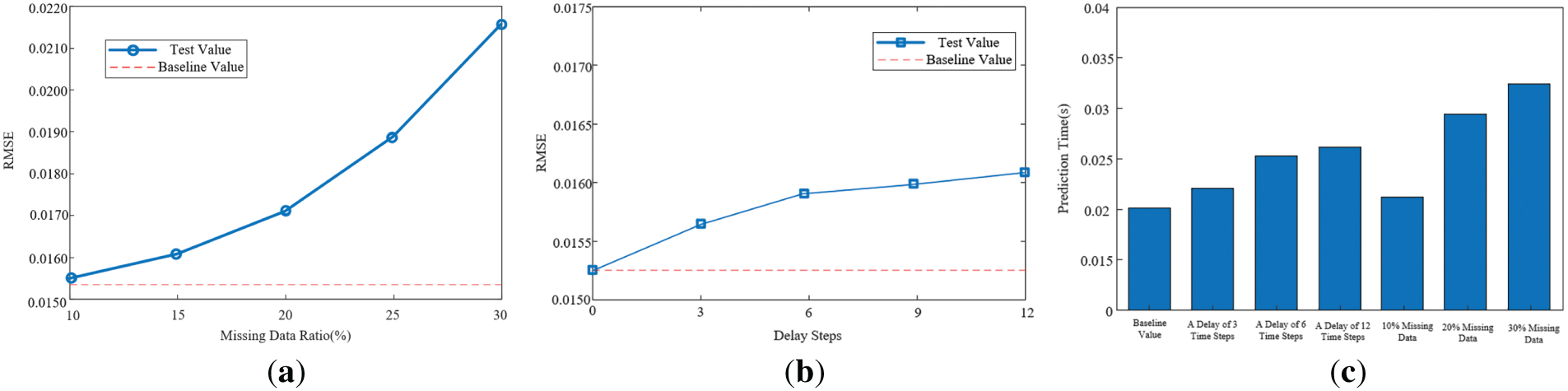
Figure 21: Test results under disturbances. (a) Missing data testing; (b) Communication delay simulation testing; (c) Prediction time under different situations

As shown in Fig. 21a,b, although the RMSE values increased slightly after testing, the fluctuations were not significant and did not affect the accuracy of the model’s output. Furthermore, Fig. 21c demonstrates that the output time under test conditions remained very close to the original time, with the average output time still being very fast. Therefore, these tests verify that the proposed model exhibits strong robustness under disturbances.

7  Conclusion

This paper addresses the challenges of transient voltage assessment and control in traditional hybrid AC/DC power systems by proposing an intelligent response model that integrates physical mechanisms with neural networks, optimized using ISAO for CNN-BiGRU. By extracting highly interpretable response characteristics and analyzing the synergistic advantages of integrating ISAO with neural networks, the effectiveness and accuracy of the method are validated through simulations. The main conclusions are as follows:

(1) For low-voltage instability scenarios in hybrid AC/DC systems, three types of characteristic response data were extracted: the P-I change rate, the integral area based on voltage trajectory, and the active power at the rectifier side of the DC system. Compared with traditional methods, the artificial intelligence approach adaptively selects threshold values for the characteristic data, provides an interpretable theoretical basis, and reduces redundancy in meaningless data. And use LVSI to screen key nodes. LVSI is based on TVSI, and its calculated values are derived from dynamic time-series data, freeing itself from the limitations of traditional static indicators. This effectively solves the problem of unclear physical correlation in input features and improves training efficiency.

(2) By introducing a good point set initialization strategy and a Gaussian mutation strategy to enhance SAO, global optimization of key hyperparameters in the response characteristic-driven CNN-BiGRU model is achieved. This overcomes the local optimum trap problem of traditional parameter-tuning methods, reduces optimization time, and significantly improves the accuracy and speed of the response-driven model.

(3) Simulation analyses on the improved CEPRI-36 system and actual power grids demonstrate that the proposed ISAO-CNN-BiGRU response-driven model outperforms traditional methods in terms of transient voltage stability assessment speed, UVLS load-shedding decision-making speed, and accuracy. It enables intelligent response from rapid fault feature extraction to accurate assessment and effective control decisions, providing efficient and reliable technical support for ensuring the secure and stable operation of hybrid AC/DC systems. The proposed method possesses considerable theoretical value and engineering application prospects.

(4) The proposed method can be adapted to other types of power systems, such as those with high penetration of renewable energy or islanded microgrids, by acquiring and training on key characteristic data to obtain corresponding results. Furthermore, the method can utilize real-time data provided by devices such as Phasor Measurement Unit (PMU) and Wide-Area Measurement System (WAM) to rapidly assess system status and generate control recommendations, thereby providing decision support for dispatchers.

While the proposed method demonstrates promising results, the model’s performance is dependent on the quality and diversity of the training data, and its behavior under extreme conditions requires further investigation. It could be gradually tested and validated in real-world environments to evaluate its sustainability and economic viability. Furthermore, integrating Physics-Informed Neural Network (PINN) into the current framework could be explored to enhance the model’s generalization capability and interpretability under rare events, as well as to develop control strategies that are co-optimized with other control schemes.

Acknowledgement: The authors would like to express special thanks to State Grid Shanxi Electric Power Company.

Funding Statement: This work was supported by the State Grid Shanxi Electric Power Company science and technology project “Research on Key Technologies for Voltage Stability Analysis and Control of UHV Transmission Sending-End Grid with Large-Scale Integration of Wind-Solar-Storage Systems” (520530240026).

Author Contributions: The authors confirm their contribution to the paper as follows: Conceptualization: Rui Xu and Xueting Cheng; Methodology: Rui Xu, Xueting Cheng and Zhichong Cao; Software: Rui Xu, Xueting Cheng and Huiping Zheng; Validation: Rui Xu, Cheng Liu and Zhichong Cao; Resources: Cheng Liu; Data curation: Rui Xu and Cheng Liu; Writing—original draft preparation: Rui Xu and Xueting Cheng; Writing—review and editing: Rui Xu, Liming Bo and Cheng Liu; Supervision: Rui Xu, Xueting Cheng, Huiping Zheng and Liming Bo; Funding acquisition: Cheng Liu. All authors reviewed the results and approved the final version of the manuscript.

Availability of Data and Materials: Data available on request from the authors. The data that support the findings of this study are available from the corresponding author, Rui Xu, upon reasonable request.

Ethics Approval: Not applicable.

Conflicts of Interest: The authors declare no conflicts of interest to report regarding the present study.

References

1. Li L, Pei W, Xiao H, Deng W, Kong L. Analysis of DC voltage oscillation mechanism in AC/DC hybrid distribution system. J Eng. 2019;2019(16):1511–7. doi:10.1049/joe.2018.8482. [Google Scholar] [CrossRef]

2. Chang F, O’Donnell JJr, Su W. Voltage stability assessment of AC/DC hybrid microgrid. Energies. 2023;16(1):399. doi:10.3390/en16010399. [Google Scholar] [CrossRef]

3. Mahmoudian A, Garmabdari R, Bai F, Guerrero JM, Mousavizade M, Lu J. Adaptive power-sharing strategy in hybrid AC/DC microgrid for enhancing voltage and frequency regulation. Int J Electr Power Energy Syst. 2024;156(1):109696. doi:10.1016/j.ijepes.2023.109696. [Google Scholar] [CrossRef]

4. Li Z, He H, Wang L, Gao L, Zhang M, Fan R. A comprehensive evaluation method of DC voltage sag in medium-low voltage DC distribution system. Energy Rep. 2022;8(9):345–56. doi:10.1016/j.egyr.2022.10.140. [Google Scholar] [CrossRef]

5. Boričić A, Torres JLR, Popov M. Comprehensive review of short-term voltage stability evaluation methods in modern power systems. Energies. 2021;14(14):4076. doi:10.3390/en14144076. [Google Scholar] [CrossRef]

6. Cai X, Quan C, Chen Y. Investigation on voltage stability evaluation indicators and algorithms for power systems based on neural network algorithms. Int J Emerg Electr Power Syst. 2024;25(5):583–91. doi:10.1515/ijeeps-2023-0148. [Google Scholar] [CrossRef]

7. Suman M, Rao MVG, Ramana Rao PV. ANN based SVC FACTS controller to enhance voltage stability of multi-machine power system. Int J Innov Technol Explor Eng. 2019;8(10):381–7. doi:10.35940/ijitee.i8401.0881019. [Google Scholar] [CrossRef]

8. Li Q, Liu XF. Voltage stability assessment of complex power system based on GA-SVM. Neural Netw World. 2019;29(6):447–63. doi:10.14311/nnw.2019.29.027. [Google Scholar] [CrossRef]

9. Biswal T, Parida SK, Mishra S. A DT-CWT and data mining based approach for high impedance fault diagnosis in micro-grid system. Procedia Comput Sci. 2023;217(1):1570–8. doi:10.1016/j.procs.2022.12.357. [Google Scholar] [CrossRef]

10. Zhang Z, Qin B, Gao X, Ding T, Zhang Y, Wang H. SE-CNN based emergency control coordination strategy against voltage instability in multi-infeed hybrid AC/DC systems. Int J Electr Power Energy Syst. 2024;160:110082. doi:10.1016/j.ijepes.2024.110082. [Google Scholar] [CrossRef]

11. Wang Z, Zhang H, Li B, Fan X, Ma Z, Zhou J. An IMFO-LSTM_BIGRU combined network for long-term multiple battery states prediction for electric vehicles. Energy. 2024;309:133069. doi:10.1016/j.energy.2024.133069. [Google Scholar] [CrossRef]

12. Chettibi N, Massi Pavan A, Mellit A, Forsyth AJ, Todd R. Real-time prediction of grid voltage and frequency using artificial neural networks: an experimental validation. Sustain Energy Grids Netw. 2021;27:100502. doi:10.1016/j.segan.2021.100502. [Google Scholar] [CrossRef]

13. Mujammal MAH, Moualdia A, Wira P, Albasheri MA, Cherifi A. Novel direct power control based on grid voltage modulated strategy using artificial intelligence. Smart Grids Sustain Energy. 2024;9(2):37. doi:10.1007/s40866-024-00225-1. [Google Scholar] [CrossRef]

14. Xu Y, Dong ZY, Meng K, Yao WF, Zhang R, Wong KP. Multi-objective dynamic VAR planning against short-term voltage instability using a decomposition-based evolutionary algorithm. IEEE Trans Power Syst. 2014;29(6):2813–22. doi:10.1109/tpwrs.2014.2310733. [Google Scholar] [CrossRef]

15. Deng L, Liu S. Snow ablation optimizer: a novel metaheuristic technique for numerical optimization and engineering design. Expert Syst Appl. 2023;225(1):120069. doi:10.1016/j.eswa.2023.120069. [Google Scholar] [CrossRef]

16. Cao Z, Liu C, Cai G. Coordination control strategy for transient voltage partitioning based on response data. Electr Power Autom Equip. 2025;6:164–72. (In Chinese). doi:10.16081/j.epae.202412013. [Google Scholar] [CrossRef]

17. Taylor CW, Erickson DC, Martin KE, Wilson RE, Venkatasubramanian V. WACS-wide-area stability and voltage control system: R&D and online demonstration. Proc IEEE. 2005;93(5):892–906. doi:10.1109/JPROC.2005.846338. [Google Scholar] [CrossRef]

18. Halpin SM, Harley KA, Jones RA, Taylor LY. Slope-permissive under-voltage load relay for delayed voltage recovery mitigation. IEEE Trans Power Syst. 2008;23(3):1211–6. doi:10.1109/tpwrs.2008.926409. [Google Scholar] [CrossRef]

19. Yang H, Li N, Sun Z, Huang D, Yang D, Cai G, et al. Real-time adaptive UVLS by optimized fuzzy controllers for short-term voltage stability control. IEEE Trans Power Syst. 2022;37(2):1449–60. doi:10.1109/TPWRS.2021.3105090. [Google Scholar] [CrossRef]

20. Li Z, Yan J, Liu Y, Liu W, Li L, Qu H. Power system transient voltage vulnerability assessment based on knowledge visualization of CNN. Int J Electr Power Energy Syst. 2024;155:109576. doi:10.1016/j.ijepes.2023.109576. [Google Scholar] [CrossRef]

21. Deng X, Hu Y, Jia Y, Peng M. Power system stability assessment method based on GAN and GRU-Attention using incomplete voltage data. IET Gener Transm Distrib. 2023;17(16):3692–705. doi:10.1049/gtd2.12925. [Google Scholar] [CrossRef]

22. Wang Y, Li Y, Li H. Snow ablation-based risk assessment method for cascading failures in an AC-DC hybrid power grid. Power Syst Protect Cont. 2025;53(4):37–47. (In Chinese). doi:10.19783/j.cnki.pspc.24617310.1109/tencon.2018.8650505. [Google Scholar] [CrossRef]

23. Zhu F, Li G, Tang H, Li Y, Lv X, Wang X. Dung beetle optimization algorithm based on quantum computing and multi-strategy fusion for solving engineering problems. Expert Syst Appl. 2024;236(1):121219. doi:10.1016/j.eswa.2023.121219. [Google Scholar] [CrossRef]

24. Lu Z, Fei Z, Wang B, Yang F. A feature fusion-based convolutional neural network for battery state-of-health estimation with mining of partial voltage curve. Energy. 2024;288:129690. doi:10.1016/j.energy.2023.129690. [Google Scholar] [CrossRef]

25. Zhao S, Zhang T, Cai L, Yang R. Triangulation topology aggregation optimizer: a novel mathematics-based meta-heuristic algorithm for continuous optimization and engineering applications. Expert Syst Appl. 2024;238:121744. doi:10.1016/j.eswa.2023.121744. [Google Scholar] [CrossRef]