CFD-Based Optimization of a Shell-and-Tube Heat Exchanger

1  Introduction

Rapid science and technological development have injected new vitality into various industries. However, the energy shortage caused by overexploitation of natural resources, surging per capital Energy Consumption (EC), and wasted energy has also hindered sustainable industrial development. Under such a backdrop, enhancing heat transfer in thermodynamics has become a research hotspot. It might provide enlightenment for protecting the ecological environment by reducing EC and improving economic benefits [1]. Meanwhile, in response to the needs of expanding production scale and refining production level, the heat transfer efficiency of the Heat Exchanger (Exchanger) must be improved. Thus, high-efficiency Exchanger has attracted extensive attention in energy conservation scenarios [2] by transferring and exchanging heat and energy between different media and fluids. A practical application of Exchanger is improving the Energy Utilization Rate (EUR), such as in aerospace, petrochemical, electric energy, and other fields. On the other hand, the advancement of new material technology has promoted the renewal of Exchanger in type, structure, power, and production capacity. As a prime example of Exchanger, Shell-and-Tube Heat Exchangers (STHEs) are tubular, highly adaptive, high-temperature proof, and high pressure resistant. They can operate stably in complex scenes. At the same time, it has a stable structure, readily available materials, simple assembly, convenient operation, high efficiency, and high reliability. Therefore, it has exerted excellent energy-saving potential in various industrial production and is seeing a significant market share [3].

In recent years, the research on Exchanger numerical simulation has developed rapidly. Iswantoro et al. [4] simulated the STHE model and studied its performance. Bellahcene et al. [5] found that the baffle increased the heat exchange area of STHE through numerical simulation. Luo et al. [6] numerically simulated the STHE using Fluent’s fluid simulation software. They obtained the cloud diagrams of temperature, velocity, and pressure fields on the shell side of tube-sheet-fixed Exchanger with different diaphragm spacing. Gao et al. [7] analyzed the influence of flow field distribution and Heat Transfer Efficiency (HTE) on STHE through numerical simulation.

Therefore, the numerical simulation technique has dramatically promoted the overall Exchanger performance. However, there are few studies on the Exchanger’s in-tube heat transfer mechanism through numerical simulation. Against such a background, the present work explicates the history and structure of Exchange. It numerically models the in-tube heat transfer mechanism pertaining to the gas-phase circulatory STHE based on aerodynamics and Engineering Fluid Mechanics (EFM). Afterward, the numerical simulation results are verified and analyzed to describe the relationship between the Exchanger tube parameters and the heat transfer performance. The present work innovatively used numerical simulation to model the Exchanger heat transfer to optimize the Exchanger performance and improve economic benefits. The research findings have practical significance and reference value for promoting heat transfer research in Exchanger tubes.

2  Theory and Method of Exchanger in-Tube Heat Transfer Simulation Based on Aerodynamics and EFM

2.1 Structure and Working Principle of Exchanger

According to application purposes, Exchangers can be divided into floating head Exchangers, U-shaped tube-sheet Exchangers, plate Exchangers, and tube-sheet-fixed Exchangers. According to heat transfer modes and principles, Exchangers can be divided into inter wall Exchanger, regenerative Exchanger, compound Exchanger, and hybrid Exchanger. The inter wall Exchanger is subdivided into the tube heat Exchanger, plate heat Exchanger, and surface expansion Exchanger. The inter wall Exchanger is the most widely used because of its good adaptability [8,9].

Most STHEs are simple in structure, easy to assemble, inexpensive, stable, and robust against extreme environments. Hence, it is favored in industrial production [10]. Fig. 1 displays the composition and working principle of the STHE.

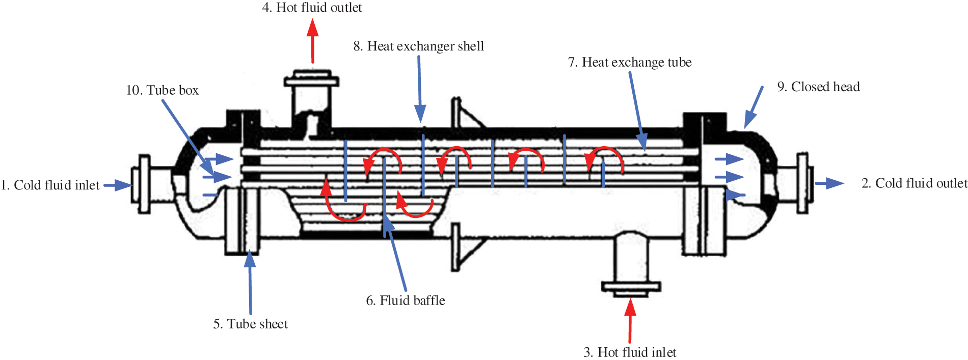
Figure 1: Structure and working principle of STHE

As in Fig. 1, the cold fluid reaches outlet 2 from inlet 1 through tube 7 during a heat exchange (tube side). The hot fluid reaches outlet 4 from inlet 3 through the interior of shell 8 and baffle 6 (the shell side).

2.2 Analysis of Related Concepts

1)   Aerodynamics

Aerodynamics is a branch of mechanics based on fluid mechanics. It is mainly used in the aviation industry to study the gas flow, force characteristics, and physical change laws of aircraft or similar objects under the same air medium or other gas media. Aerodynamic fluid inlet distributor can effectively distribute tube inlet fluid and the fluid flow velocity evenly to avoid diversion or dead zone. Theoretically, doing so can fundamentally curb tube overheating or coking. In practice, however, it is difficult to achieve such effects. Thus, people often use Computational Fluid Dynamic (CFD) software to simulate Exchanger heat transfer to predict potential tube overheating and coking. As a result, CFD modification software has become one of the most widely used modeling approaches for optimizing Exchangers [11,12].

2)   EFM

Fluid mechanics studies the mechanical laws and fluid phenomena of liquids, gases, and other fluids at rest and in motion. The research objects include the state of the fluid itself (static and moving) under different forces and the laws between fluids and between fluid and tube walls. EFM, or fluid mechanics, strives is to solve the practical problems in industrial production without much tightness requirements, and EFM theory is based on Newton’s law of motion. It abides by Mass Conservation, Momentum Conservation, and Energy Conservation laws [13,14].

3)   Finite Element Analysis (FEA)

Essentially, FEA approximately simulates the infinite unknowns of actual working conditions with a finite number of simple, independent, and interrelated unknowns through mathematical means [15]. FEA is based on discretization and deals with continuous media problems. It can simplify complex problems and provide straightforward solutions. FEA method develops rapidly and is seeing broad applications in various fields with the popularization and development of computers [16].

Here, ANSYS simulation software is used for FEA. It is the fastest growing and most popular computer-aided engineering software worldwide with excellent scalability and simple operation. The software has a three-module structure. The preprocessing module includes solid modeling, meshing, and load application. In particular, the powerful solid modeling and meshing tools can assist users in constructing finite element models. Then, the analysis and calculation module covers structural analysis and fluid mechanics analysis, among other analysis means. IT can simulate physical media interaction and be used for sensitivity analysis and optimization analysis. Lastly, the post-processing module can visualize the calculation results through color contour, gradient, or charts and curves. Fig. 2 displays the main analysis flow.

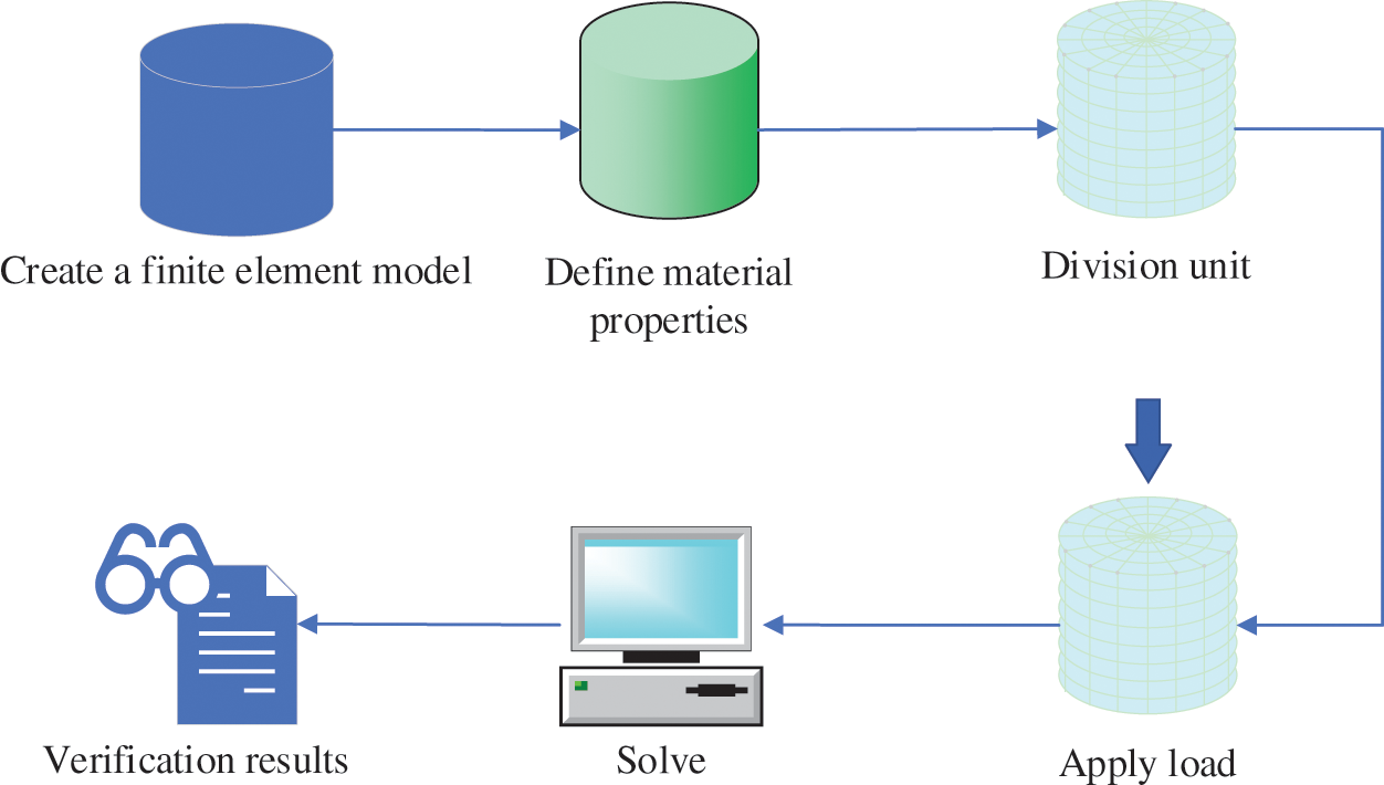
Figure 2: Flowchart of ANSYS software analysis

4)   Meshing

Meshing divides the research model into more minor elements, usually through four approaches to guarantee subsequent FEA. Firstly, the transformation expansion can mesh regular surfaces. By comparison, curve-closed fields meshing or local optimization can choose the Delaunay triangle method. Thirdly, the covering method utilizes the quadrilateral element to mesh the complete cutting curve-encircled surface. Lastly, the frontier rule divides surfaces through quadrilateral and triangular elements. Fig. 3 is the main flow of meshing.

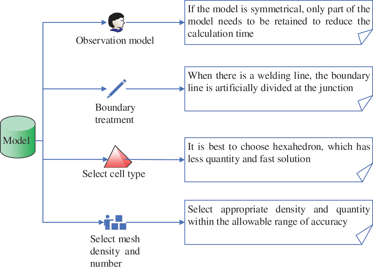
Figure 3: Flowchart of meshing

2.3 Numerical Simulation Modeling for Gas-Phase Circulatory STHE

The Exchanger structure is complicated with the continuous updating of the equipment, which makes the simulation more complex. Bruce and Peaceman proposed a new numerical simulation method in 1953, using FEA and finite volume analysis [17]. They used computers for numerical calculation and image display to solve industrial production problems. Compared with the traditional method, this has significant advantages: high flexibility, strong adaptability, low cost, and specific and intuitive display [18–20]. The finite volume analysis method, based on the conservation equation in integral form rather than a differential equation, is a commonly used numerical algorithm in computational fluid dynamics. The conservation equation in integral form describes each control volume defined by the computational grid. The finite volume method focuses on constructing discrete equations from the physical point of view. Each discrete equation expresses the conservation of a specific physical quantity on a finite volume. The physical concept of the derivation process is clear. The coefficients of the discrete equations have a certain physical significance. They can ensure that the discrete equations have conservation characteristics. The basic idea is to divide the calculation area into a series of non-repeated control volumes. Each control volume is represented by a node. The conservation differential equation to be solved integrates space and time in any control volume and a certain time interval. Then, assumptions are made about the time and space change curve or interpolation method of the function to be solved and its derivatives. Finally, each item in the first idea is integrated according to the selected profile and sorted into discrete equations about the unknown quantities on the nodes.

Next, EFM theory and aerodynamics simulate the gas-phase circulatory STHE in-tube heat transfer. The results are analyzed and verified to determine the relationship between tube parameters and heat transfer performance. A circulatory blade is added to the ordinary STHE. The circulatory blade swirls the shell side flue gas to become less adhesive and non-depositional under gravity. Meanwhile, 48 triangular heat transfer tubes can maximize transfer area and prolong transfer time. The heat transfer process complies with the three Laws of Mass Conservation, Momentum Conservation, and Energy Conservation. Now that the fluid flows as a turbulent, it follows the turbulence model [21,22].

1)   Establishment of a numerical simulation model

a.   Calculation of heat transfer

According to Newton’s cooling law, the heat transfer of hot air on the shell side is:

Qr=crqm(t2−t1) (1)

qm=qrv∗ρr (2)

In Eqs. (1) and (2), Qr indicates the heat transfer, and cr denotes the specific heat capacity of the hot fluid. qrv is the mass flow of the hot fluid. t1 and t2 represent the inlet and outlet temperatures of the shell side hot fluid, respectively. ρr stands for the hot fluid density. The specific heat capacity cr and density ρr of hot fluid are obtained by looking up the table. Then, qrv , t1 , and t2 are measured in real-time during the experiment.

b.   Calculation of logarithmic mean temperature difference on the shell side

Δtm=Δtmax−ΔtminlnΔtmaxΔtmin (3)

Δtmax=tr′−tl′′ (4)

Δtmin=tr′′−tl′ (5)

In Eqs. (3)–(5), Δtmax and Δtmin are the maximum and minimum temperature difference, respectively; tr′ and tr′′ mean the inlet and outlet temperature of hot air, respectively. tl′ and tl′′ refer to the inlet and outlet temperature of cold air, respectively.

c.   Calculation of resistance coefficient

f=ΔP12ρv∗d (6)

ΔP is the shell side pressure drop by Pa. ρ signifies the fluid density by Kg/m3. v stands for the fluid velocity by m/s. d reflects the equivalent diameter by mm.

Reynolds number: Re

Re=ρvdμ (7)

In Eq. (7), μ is the fluid viscosity coefficient by Pa⋅s .

The heat transfer’s maximum absolute error is counted to determine the heat transfer Qr , as in Eq. (8):

|δQr|=crρrqrv2(δtr′)2+qrv2(δtr′′)2+(δvr)2(tr′′−tr′)2 (8)

In Eq. (8), δtr′ , δtr′′ , qrv2 , and δQr are the maximum errors of hot air inlet temperature, outlet temperature, flow rate, and heat transfer, respectively.

Hence, the maximum relative error of heat transfer is

E(δQr)max=|δQrQr|=(δt2)2+(δt1)2(tr′′−tr′)2+(δvrvr)2 (9)

Similarly, the maximum relative errors of Δtmax and Δtmin can be obtained

E(δ(Δtmax))=|δ(Δtmax)Δtmax|=(δtr′)2+(δtl′′)2(tr′−tl′′)2 (10)

E(δ(Δtmin))=|δ(Δtmin)Δtmin|=(δtr′′)2+(δtl′)2(tr′′−tl′)2 (11)

Hence, the maximum relative error of logarithmic average temperature difference Δtm is:

E(δ(Δtm))=|δ(Δtm)Δtm|=(ΔtmaxΔtmax−Δtmin−1lnΔtmaxΔtmin)2(δ(Δtmax)Δtmax)2+(1lnΔtmaxΔtmin−ΔtminΔtmax−Δtmin)2(δ(Δtmin)Δtmin)2 (12)

d.   Governing equation

Mass conservation equation:

∂u∂x+∂v∂y+∂w∂z=0 (13)

Momentum conservation equation:

x-direction:

ρ(∂u∂t+u∂u∂x+v∂u∂y+w∂u∂z)+∂P∂x=μ(∂2u∂x2+∂2u∂2u∂y2∂z2)+gxρ (14)

y-direction:

ρ(∂v∂t+u∂v∂x+v∂v∂y+w∂v∂z)+∂P∂y=μ(∂2v∂x2+∂2v∂2v∂y2∂z2)+gyρ (15)

z-direction:

ρ(∂w∂t+u∂w∂x+v∂w∂y+w∂w∂z)+∂P∂z=μ(∂2w∂x2+∂2w∂2w∂y2∂z2)+gzρ (16)

Energy conservation equation:

ρcp(∂T∂t+u∂T∂x+v∂T∂y+w∂T∂z)=λ(∂2T∂x2+∂2T∂2T∂y2∂z2)+Q (17)

In Eqs. (13)–(17), u, v, and w are the components of the velocity vector in the x, y, and z directions, respectively, measured by m/s−1. gx , gy , and gz represent the gravity acceleration, respectively, which can be ignored. ρ is the fluid density (determined by Boussinesq approximation), in kg/m−3. μ denotes the sum of molecular viscosity and turbulent viscosity coefficient, in Pa⋅s . P indicates the pressure, in Pa. cp signifies the specific heat capacity at constant pressure, in J/(kg⋅K)−1 . λ stands for the thermal conductivity, in W/(m⋅K)−1 . t means the time, in s. T refers to the temperature, in K.

Standard k−ε model equation:

∂∂t(ρk)+∂∂xi(ρkui)=∂∂xj[(μ+μtσk)∂k∂xj]+Gk+Gb−ρε−YM+Sk (18)

∂∂t(ρε)+∂∂xi(ρεui)=∂∂xj[(μ+μtσε)∂ε∂xj]+C1εεK(Gk+C3εGb)−C2ερε2k+Sε (19)

In Eqs. (18) and (19), k is turbulent kinetic energy. ε denotes the energy dissipation rate of turbulent flow. Gk referes to the turbulent kinetic energy generated by the average velocity gradient. Gb indicates the buoyancy turbulent kinetic energy. YM means the contribution of fluctuating expansion to the total dissipation rate in compressible turbulence. ∂k and ∂ε are the turbulent Prandtl constant of k and ε . Sk and Sε mean a user-defined source item. The remaining parameters share the same meaning as the above equations.

According to the above equations, the expression of turbulent viscosity μt can be obtained

μt=ρCμk2ε (20)

2)   Physical modeling and meshing

Subsequently, an experiment is designed to simulate the gas-phase circulatory STHE. The STHE physical structure includes a hot air inlet and outlet, cold air inlet and outlet, motor, tube bundle, and a spiral blade. Fig. 4 draws the physical model diagram of the gas-phase circulatory STHE.

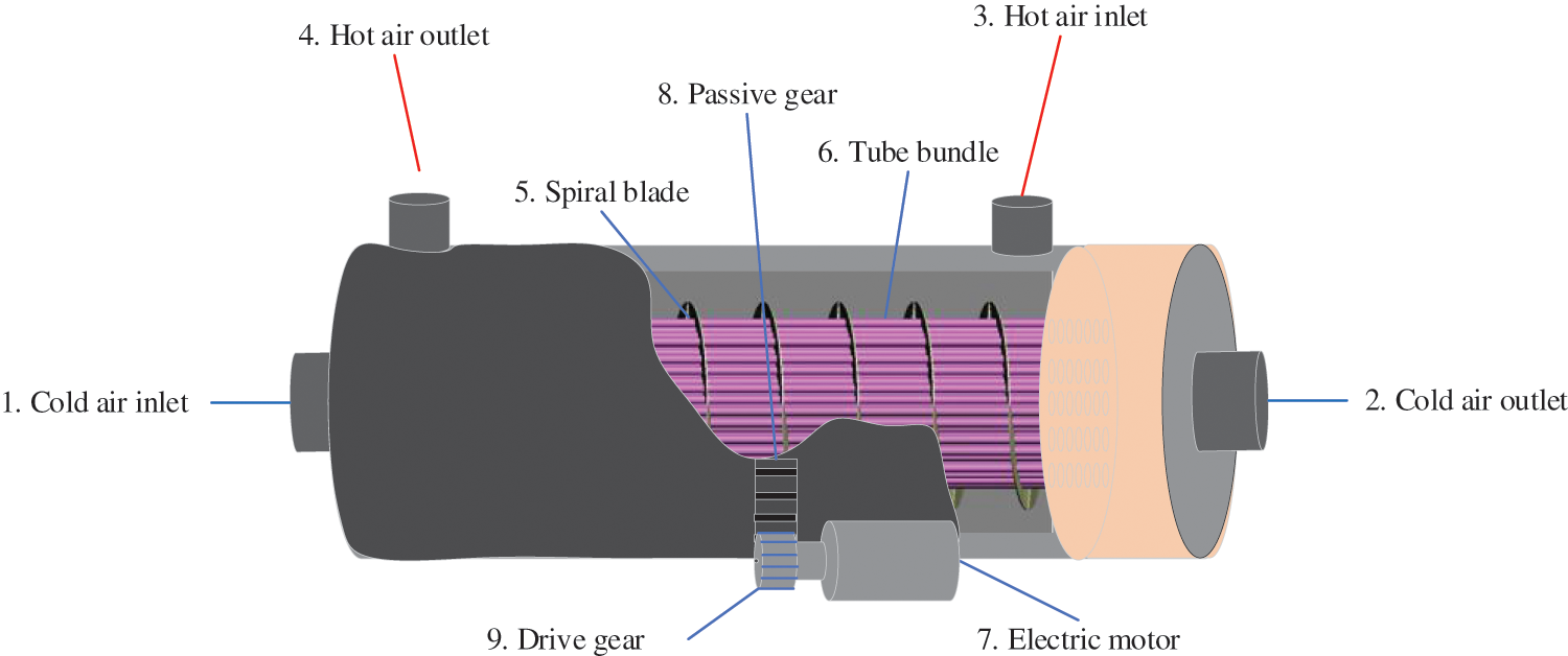
Figure 4: Schematic diagram of the physical model of gas-phase circulatory STHE

It is essential to simplify the mechanical structure of the gas-phase circulatory STHE into an FEA-meshable model and extract the solution domain in the complex geometric machinery before studying its heat transfer mechanism. Then, the solution domain is divided into finite independent elements and is connected to the nodes. Each independent element can be subdivided into different sizes for researching complex structured equipment. The meshing quality of FEA determines the accuracy of subsequent experimental results. Meshing is usually divided into structured and unstructured meshing to calculate different equipment areas. Importantly, fluid regions meshed differently will generate a different number of meshes. Besides, the mesh might get too large to model the fluid flow under different calculation accuracy correctly. However, hardware requirements, such as computer Central Processing Unit (CPU) and Random Access Memory (RAM), will surge to get the more refined mesh. Then, the cost will hike [23,24]. Therefore, practical scenarios often refine meshing by weighing cost and experimental expectations. Here, the ANSYS simulation software is employed to extract the fluid passing through the physical model and mesh the simplified model. Based on this, the present work studies the in-tube heat transfer of gas-phase circulatory STHE [25]. Fig. 5 is a partial view of meshing.

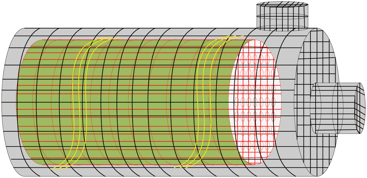
Figure 5: Partial meshing of gas-phase circulatory STHE

2.4 Experimental Design of Simulation Verification

In this section, an experiment is designed to verify the reliability of numerical simulation of Exchanger in-tube heat transfer based on aerodynamics and EFM and to study the heat transfer performance of STHE [26]. Therefore, according to the working principle of the Exchanger, the hot air circulation on the shell side and the cold air circulation on the tube side are carried out in stages. Then, the other boundary conditions are set. Finally, the experimental results are compared with the numerical simulation results [27].

1)   Construction of experimental platform

The effects of tube height, thickness, and spacing on heat transfer are verified. Therefore, different experimental platforms select specific tube parameters for gas-phase circulatory STHE [28]. Table 1 lists the specific parameters.

In careful consideration of resource benefits, an experimental platform is built according to Table 1.

Then, model heat transfer experiments are carried out with different specifications to collect experimental data comprehensively.

2)   Data acquisition system

Next, different parameters and control systems are used to collect wind speed, inlet, outlet temperature, and differential pressure [29], as shown in Table 2.

3)   Boundary condition setting

Inlet and outlet boundary setting: the test fluid is set as incompressible gas, and the inlet and outlet wind speed is set as 3∼12 m/s. The cold and hot air temperatures are initialized to 10°C and 100°C, respectively. The velocity direction is perpendicular to the inlet and outlet boundaries. The average static pressure at the inlet and outlet is 0 Pa.

Wall boundary setting: all mechanical structures of the Exchanger are closely and smoothly connected to ensure zero leakage and constant tube wall temperature so that external heat conduction can be ignored.

4)   Test procedure

Fig. 6 shows the specific simulation and verification experiment steps.

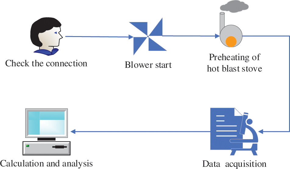
Figure 6: Flowchart of simulation verification experiment steps

First, check the tubes and the data acquisition system for possible incorrect connections or leaks. Under a normal power supply, the computer control interface can facilitate real-time monitoring.

Next, turn on the inlet blower to deliver the cold air at the speed of 6 m/s and heat it to 10°C to the Exchanger tube until the speed and temperature stabilize. Turn on the power supply of the hot blast stove and continue heating until the air temperature reaches 150°C and the airflow is stable. On the other hand, the hot air inlet is set to four gradients of 3, 6, 9, and 12 m/s as required. Then, the temperature and pressure drop is recorded at the inlet and outlet at different wind speeds. At the same time, the experimental results are monitored on the computer screen until all parameters are stable. Altogether, ten experimental results of each gradient are recorded, and the average value is taken as the final result of the gradient experiment [30].

It is important to turn off the power supply of the hot air fan, hot air stove, and cooling fan to restore the air and Exchange tubes to their original state. Finally, the collected data will be counted and analyzed by computer to complete the experiment.

3  Results and Analysis of Numerical Simulation Model

3.1 Meshing Verification Analysis

Gradients are set as per the mesh number. The temperature change determines the optimal mesh number under different meshing conditions. Fig. 7 outlines the meshing independence verification.

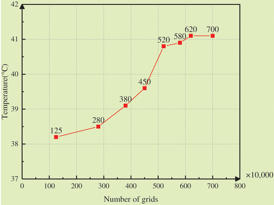
Figure 7: Verification of meshing independence

Fig. 7 reveals that the Exchanger temperature increases gradually with the mesh number. Once the mesh number surpasses 1.25 million, the Exchanger temperature increases gradually with the mesh number, raising the acceleration. Then, the temperature change stabilizes when the mesh number reaches about 5.2 million and is thus considered the optimal mesh number. Besides, the Exchanger’s mesh-variant temperature suggests that the mesh number has little impact on the final result, only within 4°C fluctuations.

3.2 Temperature Field Analysis of the Numerical Simulation Model

Fig. 8 demonstrates the simulated and analog temperature changes under different wind speeds.

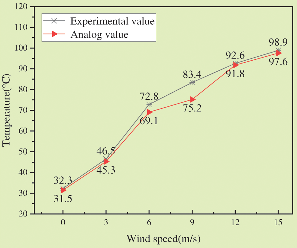
Figure 8: Temperature change curve with wind speed

As in Fig. 8, the analog and simulated value trends are roughly the same. The temperature field of the model changes fastest and slowest when the wind speed at the hot air inlet is 6 and 9 m/s, respectively. The analog and experimental results indicate that the minimum heat transfer error is 5.1% when the wind speed reaches 6 m/s. The maximum error (9.87%) occurs at a 9 m/s wind.

The pressure of the fluid also changes with the change in wind speed. Fig. 9 describes the changes in simulated and analog pressure drops under different wind speeds.

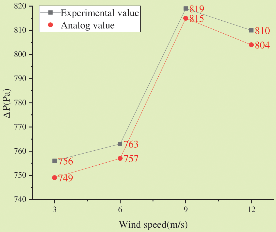
Figure 9: Curve of pressure drop with wind speed

As in Fig. 9, the pressure drop ΔP gradually increases with the wind speed under four different wind speeds. The Exchanger tube’s maximum thermal pressure drop--819 Pa--happens under a 9 m/s wind, decreasing when the wind speed reaches 12 m/s. Comparing the simulated values indicates that the pressure error has decreased by 3.32%.

The initial temperature of the hot inlet air is set at 32°C when the Exchanger tube is thermostatic. The tube wall is 100°C, and the Reynolds number Re is 35,000, 45,000, 55,000, 65,000, 75,000, 85,000 and 95,000. Then, the STHE model is numerically simulated with different spiral blade spacing and inner and outer shell diameters. Finally, the temperature field of the shell side fluid is obtained.

Fig. 10 sketches the variation of heat transfer coefficient and pressure drop on the shell side with Reynolds number.

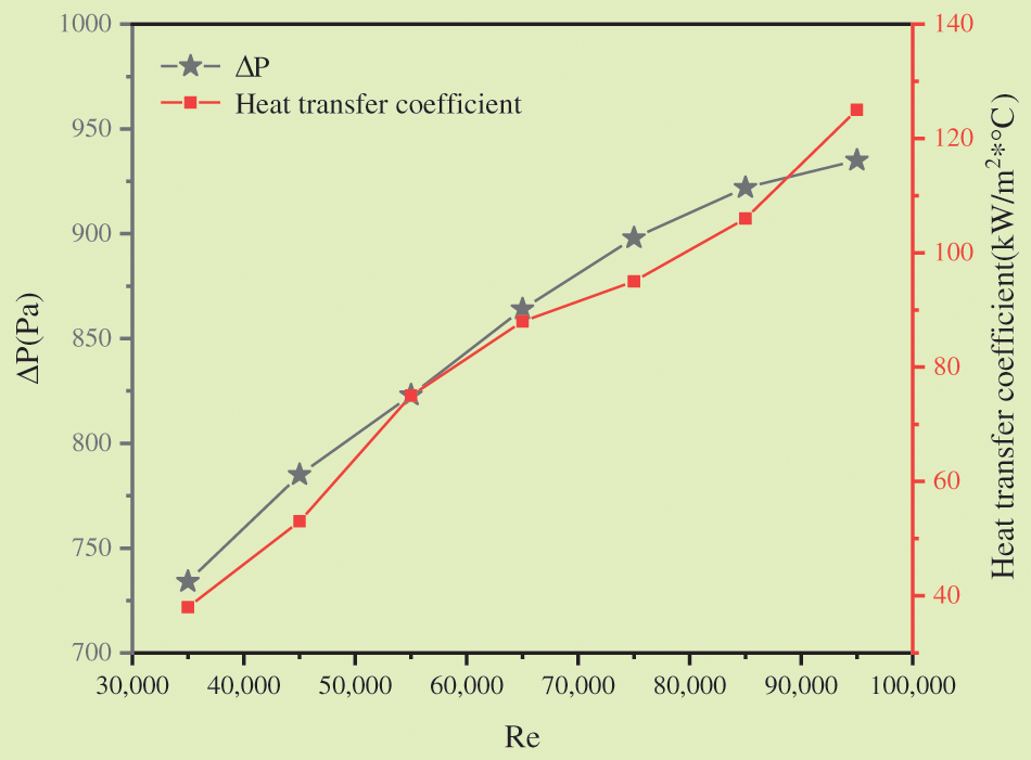
Figure 10: Variation curve of heat transfer coefficient and pressure drop with reynolds number

As in Fig. 10, under a constant temperature, the pressure drop ΔP and heat transfer coefficient of the Exchanger increase synchronously with the Reynolds number. The pressure drop change ΔP slows down when the Reynolds number reaches about 85,000. The heat transfer coefficient fluctuates continuously and rises as a whole. Thus, the pressure drop ΔP and heat transfer coefficient positively correlate with the Reynolds number.

Subsequently, Exchanger parameters are set differently to determine parameter influence on heat transfer coefficient. Fig. 11 plots the variation of heat transfer coefficient with Exchanger parameters.

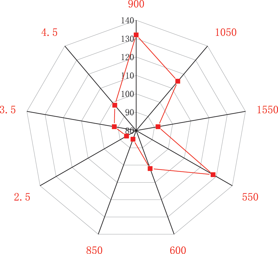
Figure 11: Variation curve of heat transfer coefficient with exchanger parameters

As in Fig. 11, the heat transfer coefficient changes with such parameters as the inner diameter of the Exchanger tube, the thickness of the tube shell, and the spacing of the spiral blades.

The heat transfer coefficient of the Exchanger increases slowly with the tube diameter, with a slight fluctuation range. By comparison, the heat transfer coefficient of the Exchanger decreases significantly with the tube’s inner diameter and the spiral blades’ spacing. Therefore, the tube’s inner diameter and the spiral blades’ spacing significantly influence the heat transfer coefficient. In simpler terms, the Exchanger heat transfer is related to its parameter specifications.

4  Conclusion

Thermodynamic heat transfer technology through Exchanger applications might provide a new direction for energy-saving solutions. Researchers have recently focused on the Exchanger performance optimization with numerical simulation technology. The present work strives to bridge the numerical simulation-based Exchanger optimization research gap by improving the Exchanger in-tube heat transfer efficiency pertaining to the gas-phase circulatory STHE tube based on aerodynamics and EFM. Then, the proposed simulation model is verified through experiments. The research findings are as follows. (1) The temperature field of the proposed STHE in-tube heat transfer model changes fastest and slowest under a tube inlet wind speed of 6 and 9 m/s, respectively. (2) The pressure drop increases first and then decreases with the wind speed, reaching the maximum at a 9 m/s wind. (3) The temperature increases with the wind speed. The closer the fluid is to the tube, the lower the temperature is at different wind speeds. (4) The pressure drop and heat transfer coefficient of the STHE increase simultaneously with the Reynolds number. The Exchanger heat transfer performance is influenced by tube height, thickness, and spiral blade spacing. Finally, the research shortcomings are pointed out. The proposed model only considers four wind speeds. Further simulation on different wind speeds will be conducted in the follow-up research. This exploration contributes to optimizing Exchanger tube heat transfer and provides a theoretical reference for relevant research.

Funding Statement: The authors received no specific funding for this study.

Conflicts of Interest: The authors declare that they have no conflicts of interest to report regarding the present study.

References

1. Islam, M. S., Saha, S. C. (2021). Heat transfer enhancement investigation in a novel flat plate heat exchanger. International Journal of Thermal Sciences, 161(3), 106763. [Google Scholar]

2. Mehrpooya, M., Dehqani, M., Mousavi, S. A. (2022). Heat transfer and economic analyses of using various nanofluids in shell and tube heat exchangers for the cogeneration and solar-driven organic rankine cycle systems. International Journal of Low-Carbon Technologies, 17(8), 11–22. https://doi.org/10.1093/ijlct/ctab075 [Google Scholar] [CrossRef]

3. Shang, X. S., Jia, L. (2017). On the selection standards and design of shell and tube heat exchangers. China Petroleum and Chemical Standards and Quality, 37(10), 181–182. [Google Scholar]

4. Iswantoro, A., Semin., Pitana, T., Zaman, M. B. (2021). Design of shell and tube heat exchanger for ballast water treatment applications on ships based on simulation. IOP Conference Series: Materials Science and Engineering, 1052, 012035. [Google Scholar]

5. Bellahcene, L., Sahel, D., Yousfi, A. (2021). Numerical study of shell and tube heat exchanger performance enhancement using nanofluids and baffling technique. Journal of Advanced Research in Fluid Mechanics and Thermal Sciences, 80(2), 42–55. [Google Scholar]

6. Luo, X., Chen, B., Min, M., Jin, M., Liu, H. (2021). Numerical simulation of shell and tube heat exchanger based on fluent. IOP Conference Series: Earth and Environmental Science, 791, 012084. [Google Scholar]

7. Gao, X. L., Chen, Z. G., Liu, Z. F., Guo, H. L., Meng, J. J. et al. (2019). Numerical simulation of the influence of the notch height of the shell and tube heat exchanger on the flow field. Journal of Hebei Institute of Civil Engineering and Architecture, 37(1), 115–118+123. [Google Scholar]

8. Levina, T. M., Kireeva, N. A., Zharinov, Y. A., Krasnov, N. A. (2021). Minimizing deposit formation in industrial fluid heat exchangers. IOP Conference Series: Earth and Environmental Science, 666(3), 032007. https://doi.org/10.1088/1755-1315/666/3/032007 [Google Scholar] [CrossRef]

9. Karimi, H., Ahmadi, H., Aghanajafi, C. (2021). Optimization techniques for design a shell and tube heat exchanger from an economic viewpoint. AUT Journal of Mechanical Engineering, 5(2), 313–328. [Google Scholar]

10. Zhu, G. M. (2017). Research on the working principle and structure of shell-and-tube heat exchangers. Industry and Technology Forum, 16(16), 74–75. [Google Scholar]

11. Zhang, D. S., Yang, X. J. (2019). Racing traction control system based on aerodynamics. Journal of Qingdao University of Science and Technology (Natural Science Edition), 179(4), 109–116. [Google Scholar]

12. Menni, Y., Lorenzini, G., Kumar, R., Mosavati, B., Nekoonam, S. et al. (2021). Aerodynamic fields inside S-shaped baffled-channel air-heat exchangers. Mathematical Problems in Engineering, 45(8), 7306–7313. https://doi.org/10.1155/2021/6648403 [Google Scholar] [CrossRef]

13. Wang, L., Xue, R., Zhou, X. (2020). Using fluent software to explain several knowledge points of engineering fluid mechanics. Education Modernization, 7(19), 126–130. [Google Scholar]

14. Jia, J. G. (2020). Analysis of temperature rise in high-speed permanent magnet synchronous traction motors by coupling the equivalent thermal circuit method and computational fluid dynamics. Fluid Dynamics & Materials Processing, 16(5), 919–933. https://doi.org/10.32604/fdmp.2020.09566 [Google Scholar] [CrossRef]

15. Popov, V., Kashelkin, V. V., Demidov, A. S. (2021). Assessment of the strength reliability of high-temperature heat exchangers with long service life at the design stage. Frattura ed Integrità Strutturale, 15(55), 136–144. https://doi.org/10.3221/IGF-ESIS.55.10 [Google Scholar] [CrossRef]

16. Denkenberger, D., Pearce, J. M., Brandemuehl, M., Alverts, M., Zhai, J. (2021). Expanded microchannel heat exchanger: Finite difference modeling. Designs, 5(4), 58. https://doi.org/10.3390/designs5040058 [Google Scholar] [CrossRef]

17. Bruce, G. H., Peaceman, D. W.,Rachford, H. A., Rice, J. D. (1953). Calculations of unsteady-state gas flow through porous media. Journal of Petroleum Technology, 5(3), 79–92. [Google Scholar]

18. Wang, W. S., Liu, S. (2019). Numerical simulation analysis of shell and tube heat exchanger based on FLUENT. Piping Technology and Equipment, 160(6), 34–35+59. [Google Scholar]

19. Ibrahim, M., Saleem, S., Chu, Y. M., Ullah, M., Heidarshenas, B. (2021). An investigation of the exergy and first and second laws by two-phase numerical simulation of various nanopowders with different diameter on the performance of zigzag-wall micro-heat sink (ZZW-MHS). Journal of Thermal Analysis and Calorimetry, 145(3), 1611–1621. https://doi.org/10.1007/s10973-021-10786-3 [Google Scholar] [CrossRef]

20. Jia, Y. J., Wang, J. J., Shang, L. S. (2020). Optimization of a heat exchanger using an ARM core intelligent algorithm. Fluid Dynamics & Materials Processing, 16(5), 871–882. https://doi.org/10.32604/fdmp.2020.09957 [Google Scholar] [CrossRef]

21. Zhang, S. W. (2019). Numerical simulation study of fluid flow in shell-and-tube heat exchanger. Journal of Wuxi Vocational and Technical College of Commerce, 19(3), 92–98, 102. [Google Scholar]

22. Chuan, H., Duan, Y. (2019). Heat transfer optimization of tube heat exchanger in mixed gas waste heat recovery. Journal of Chongqing University, 42(4), 86–95. [Google Scholar]

23. Shang, L., Jia, Y., Zheng, L., Shi, E., Sun, M. (2022). A genetic algorithm for optimizing yaw operation control in wind power plants. Fluid Dynamics & Materials Processing, 18(3), 511–519. https://doi.org/10.32604/fdmp.2022.017920 [Google Scholar] [CrossRef]

24. Xue, Z. X. (2020). Finite element analysis and strain test study of plate heat exchanger frame. Chemical Equipment and Piping, 316(1), 45–50. [Google Scholar]

25. Zheng, S., Yaln, Y., Liu, S., Xia, M., Li, S. (2022). Optimization of a high-pressure water-powder mixing prototype for offshore platforms. Fluid Dynamics & Materials Processing, 18(3), 537–548. https://doi.org/10.32604/fdmp.2022.018500 [Google Scholar] [CrossRef]

26. Qian, X., Lee, S. W., Yang, Y. (2021). Heat transfer coefficient estimation and performance evaluation of shell and tube heat exchanger using flue gas. Processes, 9(6), 939. https://doi.org/10.3390/pr9060939 [Google Scholar] [CrossRef]

27. Sundari, S. (2021). Void fraction features using image processing on a clear capillary pipe with a 45° slope to the horizontal line of two-phase air-liquid flow with high viscosity. Journal of Advanced Research in Fluid Mechanics and Thermal Sciences, 83(2), 164–172. [Google Scholar]

28. Xie, Q., Liang, C., Fu, Q., Wang, X., Liu, Y. (2022). Numerical investigation on heat transfer performance of molten salt in shell and tube heat exchangers with circularly perforated baffles. Journal of Renewable and Sustainable Energy, 14(2), 023703. https://doi.org/10.1063/5.0083647 [Google Scholar] [CrossRef]

29. Malika, M., Bhad, R., Sonawane, S. S. (2021). ANSYS simulation study of a low volume fraction CuO–ZnO/water hybrid nanofluid in a shell and tube heat exchanger. Journal of the Indian Chemical Society, 98(11), 100200. https://doi.org/10.1016/j.jics.2021.100200 [Google Scholar] [CrossRef]

30. Yılmaz, M. S., Ünverdi, M., Kücük, H., Akcakale, N., Halıcı, F. (2022). Enhancement of heat transfer in shell and tube heat exchanger using mini-channels and nanofluids: An experimental study. International Journal of Thermal Sciences, 179(4), 107664. https://doi.org/10.1016/j.ijthermalsci.2022.107664 [Google Scholar] [CrossRef]