Unsteady Flow and Heat Transfer of a Casson Micropolar Nanofluid over a Curved Stretching/Shrinking Surface

Nomenclature

1  Introduction

COVID-19 has altered our way of life, causing us to become more aware of the limitations that we as humans confront. Scientists and clinicians around the world are scrambling to figure out what is causing the epidemic of the COVID-19 virus and what they can do to stop it. Scientists have concluded, as a result of recent investigations, that nanotechnology can be used to address a wide range of clinical difficulties, including the Coronavirus pandemic [1]. Nanotechnology has the potential to be used to prevent and identify diseases in their early stages. The nanoparticles, when introduced into human immune system, have the potential to target diseases at the cellular level. Nanoparticles have the extra advantage of delivering molecular adjuvants for loaded antigens, which can improve the efficacy and safety of a vaccine while also increasing its efficacy. In order to target delivery at the cellular level, a large number of vaccines are being produced on the basis of nanoparticles (Lipid nanoparticles). The BioNTech/Pfizer and Moderna mRNA Corona virus vaccines, for example, make use of Lipid nanoparticles to deliver treatments more efficiently to the patient. Aside from that, face masks constructed of nanomaterials are more capable of providing efficient air filtering and can also be reused for a longer period of time, giving them an added edge in overcoming the shortage of high-quality masks.

Nanotechnology operates at the nanometric scale, and as a result, it is the study of a wide range of systems and technologies that operate at this scale. Nanofluids, which are based on nanomaterials, are becoming increasingly used in a variety of industrial and technical operations. Yoo et al. [2] were the first to propose the concept of nanofluids in the year 1995, and since then, nanofluids have become a popular topic of discussion among scientists. Yoo et al. [2] investigated the prospect of increasing energy exchange among fluids by incorporating various nanoparticles into the mix. Fetecau et al. [3] developed a precise solution for the flow of nanoliquids by employing a fractional model. Meanwhile, Khan et al. [4] presented the challenge of thin film electrically guided nanoliquids sprayed over a stretching cylinder in their paper Tinny film electrically steered nanoliquids sprayed over a stretching cylinder in their paper. A study conducted by Mekheimer et al. [5] using gyrotactic suspended nanoparticles and micro organisms to investigate the discharge of Prandtl fluid flow by utilizing chemical reaction, radiation, and magnetic field effects has just been published. Meanwhile, Ahmed et al. [6] investigated the Fa lkner-Skan problem with double stratification in the flow of nanofluids by employing single/multiple wall carbon nanotubes in the flow of single/multiple wall carbon nanotubes [7]. We out a comparative investigation of ethylene glycol-based nanofluid flows, employing electro-osmotic and peristaltic pumping techniques. To examine Hybrid nanoliquid slip flows, Wahid et al. [8] used an exponentially stretching/shrinking permeable sheet that was stretched and shrunk exponentially. Because of the increasing demand for nanoliquid flows in numerous fields of research and development, we find a wealth of studies on nanoliquid flows conducted by a large number of other researchers [9,10].

Micropolar fluids are a class of non-Newtonian fluids in which we are interested in the micro-motion of fluid particles and are therefore named as such. Eringen [11] was the first to propose the concept of micro components in fluids, back in 1966. The formation of a boundary layer of micro-structured liquids, on the other hand, was predicted by Willson [12]. With the use of Lubrication approximation theory, Asghar et al. [13] were able to obtain a reduced version of the flow equation to represent Micropolar slime. In the contemporary age, Abbas et al. [14] investigated the prospect of increasing energy transformation among Micro-rotational nanoliquids by employing the Ota, Yamada, and Xue models of hybrid nanoliquids, which were developed by Ota, Yamada, and Xue. For their part, Ismail et al. [15] used generated magnetic field effects to analyze the flow of micro-structured fluids while conducting their experiments. With the help of a magnetic curved surface, Abbas et al. [16] investigated the unsteady flow of Micropolar fluid flows. Raza et al. [17] discovered dual solutions in their investigation of Micropolar fluid flows utilizing thermal radiations, which was published just a few months ago.

Casson fluid is yet another essential non-Newtonian liquid that is becoming increasingly important in our daily lives, according to the National Institute of Standards and Technology. Casson fluids include a variety of sauces, jellies, and soups, amongst other things. Casson [18] was the first to derive the constitutive equations for Casson fluid and to illustrate the properties of various polymers. He published his results in 1959. McDonald [19] pointed out in 1974 that the flow of blood is a good representation of the Casson fluid model. Under-discussed fluid classes find use in a diverse range of fields including medical, biology, the food industry, and several sorts of drilling procedures, just to name a few. Because of the wide range of applications for which this essential class of fluids is used, many researchers keep a close eye on it in their laboratories. Through the use of the homotopy approach, Nadeem et al. [20] found the optimal solutions of Casson nanoliquid flows. The authors of another paper [21] concluded that skin friction along the wall is lower in Newtonian fluids than in non-Newtonian Casson-nanofluids when comparing the two types of fluids. When it comes to the flow of Casson nanoliquids, Mustafa et al. [22] used general power law velocity dispersal to analyze the phenomenon. Sarkar et al. [23] investigated the evolution of Casson nanoliquids in the aggregation of wedge angle and melting processes, respectively. In a similar vein, Ibrar et al. [24] investigated the flow of Casson nanoliquids with magnetic current using single and multiple wall carbon nanotubes, respectively. Nayak et al. [25] used entangled motile gyrotactic micro-creatures to examine the flow of Casson nanoliquids utilizing chemical processes in order to better understand their behavior. Several researchers, including Khan et al. [26], have investigated the possibility of a dual solution in the evolution of Casson fluid flows across a Stretching/Shrinking sheet.

We believe that unsteady fluid mix is appropriate based on the literature research and to the best of our knowledge. Nanofluids flows across a curved Stretching/Shrinking surface using the Micropolar Casson-Buongiorno model have not been investigated previously. Based on the findings of the studies given in [27,28], we determined that it was reasonable to unleash the dual solution phenomena utilizing the fluid flows under consideration. Stability testing will be carried out in order to better understand and identify the most appropriate solutions that will be physically feasible. To achieve this goal, we will introduce a form of exponential function into our steady state system to represent perturbation to it. This results in the stable situation being turned into an eigen value problem, from which acceptable eigen values are selected and noted for future reference.

2  Mathematical Formulation

Consider the case of a liquid mixture. As illustrated in Fig. 1, a Casson Micropolar nanofluid is discharged across a bent stretching/shrinking surface that has been wrapped in a circle of radius R. For our two-dimensional frame of reference rs−axes , we will use the (r+R,s) Curvilinear Coordinates System as our starting point. The velocity components u and v are measured in the directions of the s and r axis, and correspondingly. It is proposed that a hydrodynamic force acting in the r direction of the surface will aid in the control of the flow of the fluid in question. When the normal assumptions for boundary layer approximations are taken into consideration, the set of equations that governs this particular flow is the following:

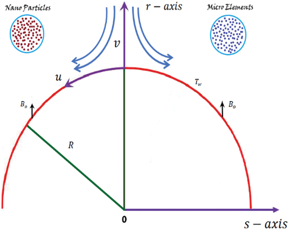
Figure 1: Geometry of the flow

∂u∂s+1R∂∂r(rv+Rv)=0, (1)

ρu2=(r+R)∂p∂r, (2)

∂u∂t+(Rur+R)∂u∂s+v∂u∂r+vu(r+R)=−(Rr+R)∂pρ∂r+ν(1β+K+1)[−u(r+R)2+∂2u∂r2+(1r+R)∂u∂r]−Kρ∂N∂r−σB0ρu, (3)

∂∂t(N)+v∂∂r(N)+RNr+R∂∂s(N)=(1+0.5K)[∂2N∂r2+(1r+R)∂N∂r]−K[(1r+R)u+2N+∂N∂r], (4)

∂T∂t+(Rur+R)∂T∂s+v∂T∂r=α1∗(∂2T∂r2+(1r+R)∂T∂r)+ρcpρcf[DB(∂T∂r)(∂C∂r)+(DTT∞)(∂T∂r)2], (5)

∂C∂t+(Rur+R)∂C∂s+v∂C∂r=DB[(1r+R)∂C∂r+∂2C∂r2]+(DTT∞)[∂2T∂r2+(1r+R)∂T∂r]. (6)

When t>0 , the relevant boundary conditions are

u=bs,v=aν,N+n(∂u∂r)=0,DB(∂C∂r)=−DTT∞(∂T∂r),atr=0,

u→0,∂u∂r→0N→0,C=C∞,T=T∞asr→∞. (7)

Eqs. (1)–(4) represent velocity and angular velocity profile, Eqs. (5) and (6) represent temperature profile and concentration of nano particles.

To simplify the above equations, we will use these transformations:

v=−(Rr+R)aν(1−αt)f(η),u=asf′(η)(1−αt),

N=(as(1−αt))aν(1−αt)g(η),

φ(η)=(C−C∞)(Cw−C∞),p=(ρa2s2P(η))(1−αt)2,

θ(η)=(T−T∞)(Tw−T∞),η=aν(1−αt)r. (8)

After solving Eqs. (2)–(6) we get

(1+1β+K)[fiv+2f′′′η+K∗−f′′(η+K∗)2+f′(η+K∗)3]−K∗η+K∗(f′f′′−ff′′′)−K∗(η+K∗)2(f′2−ff′′)−K∗(η+K∗)3ff′−K(g′′+g′η+K∗)−β∗2(3f′′+ηf′′′)−β∗η+K∗(f′+η2f′′)−M2(f′′+g′η+K∗)=0, (9)

(1+0.5K)(g′′+1η+K∗g′)+K∗η+K∗g′f−K∗η+K∗gf′′−K(2g+1η+K∗f′+f′′)−0.5β∗(3g+g′η)=0, (10)

θ″+1(η+K∗)θ′+Pr[K∗θ′fη+K∗+θ′2Nt+φ′θ′Nb−0.5ηβ∗θ′]=0, (11)

φ′′+1η+K∗φ′−Le[0.5ηβ∗φ′−K∗fη+K∗φ′]+NtNb(1η+K∗θ′+θ′′)=0. (12)

The boundary conditions for above flow problem are:

f(0)=0,f′(0)=λ,g(0)+nf′′(0)=0,θ(0)=1,Nbφ′(0)=−Ntθ′(0),

f′(η)→1,g(η)→0,f′′(η)→0,φ(η)→0,θ(η)→0,asη→∞. (13)

Moreover, some of the important physical measures are Skin friction coefficient Cf , Nusselt number Ns , Sherwood number Shs and these are expressed as:

Cf=τrsρuw2,Ns=sqwk(Tw−T∞),Shs=shmDB(Cw−C∞) (14)

where, τrs , sqw, shm are defined as:

τrs=ρ(1+K+1β)(∂u∂r+ur+R+kN)r=0,τm=ρ(1+K/2)(∂N∂r+Nr+R)r=0,qw=−(∂T∂r)r=0, (15)

Moreover, the dimensionless form these measures are:

Res1/2Cf=(1+K+1β)f′′(0)+f′(0)K*),Res−1/2Nus=−θ′(0),

Res−12Shs=−φ′(0), (16)

where Res=(as2νf) is the local Reynold number.

3  Stability Analysis

Under specified parametric combinations, the numerical simulation of Eqs. (9)–(13) yields dual solutions to the equations. It is therefore essential to choose the most appropriate solution that is both realistic and viable. The stability analysis will be conducted in accordance with the methodologies established by the authors Weidman et al. [27] and Rosca et al. [28], respectively. In order to accomplish this, we establish another variable τ=at , where is linked to the beginning value problem and thus provides us with the most likely replies between the two alternatives. We introduce some additional similarity variables:

u=as(1−αt)f′(η,t),v=−(Rr+R)a/ν(1−αt)f(η,t),

N=(as1−αt)a/ν(1−αt)g(η,t),φ(η,t)=(C−C∞)/(Cw−C∞),

p=[ρs2a2(1−αt)2]P(η,t),η=a/ν(1−αt)r,

θ(η,t)=(T−T∞)(Tw−T∞),K∗=Raν(1−αt),α=aβ1. (17)

Simplifying Eqs. (3)–(6) using transforming variables from (17) we have

(1β+K+1)[−1(K∗+η)2∂2f∂η2+∂4f∂η4+1(K∗+η)3∂f∂η+2K∗+η∂3f∂η3]−K∗K∗+η(−f∂3f∂η3+∂2f∂η2∂f∂η)−K∗(K∗+η)2[−f∂2f∂η2+(∂f∂η)2]−K∗(K∗+η)3f∂f∂η−K[∂2g∂η2+1K∗+η∂g∂η]−β∗K∗+η(∂f∂η+0.5η∂2f∂η2)−0.5β∗(η∂3f∂η3+3∂2f∂η2)−M2(∂2f∂η2+1K∗+η∂f∂η)+(αt−1)∂3f∂τ∂η2+(αt−1)K∗+η∂2f∂τ∂η=0, (18)

(1+0.5K)(1K∗+η∂g∂η+∂2g∂η2)+(K∗K∗+η)[−g∂f∂η+f∂g∂η]−0.5β∗(η∂g∂η+3g)+(αt−1)∂g∂τ−K(2g+1K∗+η∂f∂η+∂2f∂η2)=0, (19)

∂2θ∂η2+1(K∗+η)∂θ∂η+Pr[K∗K∗+ηf∂θ∂η+(∂θ∂η)2Nt+(∂φ∂η∂θ∂η)Nb−∂θ∂ηηβ∗2−(1−αt)∂θ∂τ]=0, (20)

∂2φ∂η2+(1K∗+η)∂φ∂η−Le[(∂φ∂ηηβ∗2)+(1−αt)∂φ∂τ−(K∗fK∗+η)∂φ∂η]+[1K∗+η∂θ∂η+∂2θ∂η2]NtNb=0. (21)

Subject to boundary conditions

f(0,τ)=0,n∂2f∂η2(0,τ)+g(0,τ)=0,∂f∂η(0,τ)−λ=0,

θ(0,τ)−1=0,∂φ∂η(0,τ)Nb=−∂θ∂η(0,τ)Nt.

Also, when η→∞ we have

∂f∂η(η,τ)→0,∂2f∂η2(η,τ)→0,θ(η,τ)→0,

φ(η,τ)→0,g(η,τ)→0. (22)

We have steady solution of the system of Eqs. (9)–(12) with boundary condition (13), in the form f(η)=f0(η),g(η)=g0(η),θ(η)=θ0(η) and φ(η)=φ0(η) .

We assume the following variables to generate the perturbation:

f(η,τ)=F(η,τ)e−γτ+f0(η),

g(η,τ)=G(η,τ)e−γτ+g0(η),

θ(η,τ)=H(η,τ)e−γτ+θ0(η),

φ(η,τ)=Q(η,τ)e−γτ+φ0(η), (23)

Here functions F(η,τ) , G(η,τ) , H(η,τ) and Q(η,τ) are very small as compared to f0(η),g0(η),θ0(η)andφ0(η) respectively with γ being the eigen value parameter. Simplifying Eqs. (18)–(22), by using Eq. (23) we have

(1+1β+K)[(1(K∗+η)3)∂F∂η−(1(K∗+η)2)∂2F∂η2+(2K∗+η)∂3F∂η3+∂4F∂η4]−K∗K∗+η[(∂2F∂η2)f0′+(∂F∂η)f0′′−(∂3F∂η3)f0−Ff0‴]−K∗(K∗+η)2[−(∂2F∂η2)f0−Ff0′′+2(∂F∂η)f0′]−K∗(K∗+η)3(f0∂F∂η+f0′F)+(1−αt)K∗+η[−∂2F∂η∂τ+γ∂F∂η]−β∗K∗+η(0.5η∂2F∂η2+∂F∂η)−0.5β∗(η∂3F∂η3+3∂2F∂η2)−K(1K∗+η∂G∂η+∂2G∂η2)+(1−αt)[γ∂2F∂η2−∂3f∂η2∂τ]−M2(∂2F∂η2+1K∗+η∂F∂η)=0, (24)

(1+0.5K)[(1η+K∗)∂G∂η+∂2G∂η2]+K∗η+K∗[∂G∂ηf0+g0′F−f0′G−∂F∂ηg0]−β∗2(η∂G∂η+3G)−K[(1η+K∗)∂F∂η+2G+∂2F∂η2]−(1−αt)(−γG+∂G∂τ)=0, (25)

(1η+K∗)∂H∂η+∂2H∂η2−Pr[−K∗η+K∗(∂H∂ηf0+θ0′F)−(∂Q∂ηθ0′+∂H∂ηφ0′)Nb−2∂H∂ηθ0′Nt+(−Hγ+∂H∂τ)(1−αt)+0.5ηβ∗∂H∂η]=0, (26)

(1η+K∗)∂Q∂η+∂2Q∂η2−Le[−K∗η+K∗(∂Q∂ηf0+φ0′F)+(−Qγ+∂Q∂τ)(1−αt)+0.5ηβ∗∂Q∂η]+(1η+K∗)∂H∂ηNtNb+∂2H∂η2NtNb=0, (27)

and the corresponding boundary conditions are

∂f∂η(0,τ)=0,F(0,τ)=0,G(0,τ)=−n∂2F∂η2(0,τ),

Nb∂Q∂η(0,τ)=−Nt∂H∂η(0,τ),θ(0,τ)=1.

For η→∞, we have

∂F∂η(η,τ)→0,∂2F∂η2(η,τ)→0,,H(η,τ)→0,G(η,τ)→0Q(η,τ)→0. (28)

Keeping in view the work done by authors in [27,28], we investigate the steady solutions g0(η),θ0(η) , f0(η),φ0(η) in Eqs. (9)–(12), substituting τ=0 in the system of Eqs. (24)–(28). Thus G=G0(η) , F=F0(η) , H=H0(η) , and Q=Q0(η) is considered to be the initial rise and fall in Eq. (23). After simplifications we attained the following linearized eigen value system:

(1β+K+1)[F0iv+(1(η+K∗)3)F0′−(1(η+K∗)2)F0′′+(1η+K∗)2F0‴]−(F0′′f0′+F0′f0′′−F0‴f0−F0f0‴)(K∗η+K∗)−K∗(η+K∗)2[−F0′′f0+2f0′F0′−F0f0′′]−K∗(η+K∗)3(f0′F0+F0′f0)−K[(1η+K∗)G0′+G0′′]−β∗η+K∗(F0′+0.5ηF0′′)+γη+K∗F0′−0.5β∗(3F0′′+ηF0‴)+γF0′′=0, (29)

(1+0.5K)[(1K∗+η)G0′+G0′′]+K∗η+K∗[f0G0′+F0g0′−G0f0′−g0F0′]−K∗(2G0+F0′′+1η+K∗F0′)−β∗2(ηG0′+3G0)+γG0=0, (30)

H0′′+1K∗+ηH0′−Pr[0.5ηβ∗H0′−K∗K∗+η(f0H0′+F0θ0′)−Nb(θ0′Q0′+φ0′H0′)−γH0−2Ntθ0′H0′]=0, (31)

Q0′′+Q0′(1K∗+η)−Le[−K∗K∗+η(Q0′f0+φ0′F0)−Q0γ+0.5ηβ∗Q0′]+[H0′′+(1K∗+η)H0′]NtNb=0. (32)

The boundary conditions are as follows:

F0(0)=0,F0′(0)=0,G0(0)=−nF0′′(0),

θ0(0)=0,Q0′(0)Nb=−H0′(0)Nt.

For η→∞, we have,

F0′(η)→0,F0′′(η)→0,H0(η,τ)→0,G0(η)→0,Q0(η)→0 (33)

As per findings of authors Weidman et al. [27] and Rosca et al. [28], the stability analysis will give smallest values for γ . We modify condition F0′(η)=1, to solve the system (29)–(33). Table 2 shows smallest eigen values obtained hence forth.

4  Discussion on Numerical Solutions

We will now investigate impacts of various embedded parameters on different profiles.

4.1 Velocity Profile

Velocity Profile f′(η) has two solutions, which are depicted in Fig. 2. For both solutions, we can observe that the velocity decreases as a function of the material parameter K. As a result, increasing the amount of Micropolar components in the solution can reduce the flow rate. However, when compared to the second solution, the first solution has a broader profile. According to this behavior, Micropolar components generate spin gradient viscosity, which causes the flow speed to slow down as a result of the flow. Fig. 3 depicts that the same profile lowers as the bendiness parameter K* is increased for both solutions, as seen in the graph. Due to the fact that curving the bent channel further increases the breadth of the boundary layer, which results in a drop in the flow’s speed, this phenomenon happens. On the right-hand side of Fig. 4, we can see that increasing the value of parameter causes the profile f′(η) for both solutions to be reduced. By increasing the fluid thickness, the non-Newtonian parameter creates flow regime resistivity, which results in a lowering of the profile of interest f′(η) . Both solutions flow more quickly when the magnetic indicator number M is used, as illustrated in Fig. 5. When comparing the first and second solutions, the profile of the first solution climbs significantly higher. The magnetic parameter M is in charge of regulating the speed of the flow through the system. In reality, the parameter M generates Lorentz force, which can be used to enhance the speed of the flow by acting in the direction of the flow regime. Furthermore, the same force can also be utilized to counteract the movement of the flow in the opposite direction.

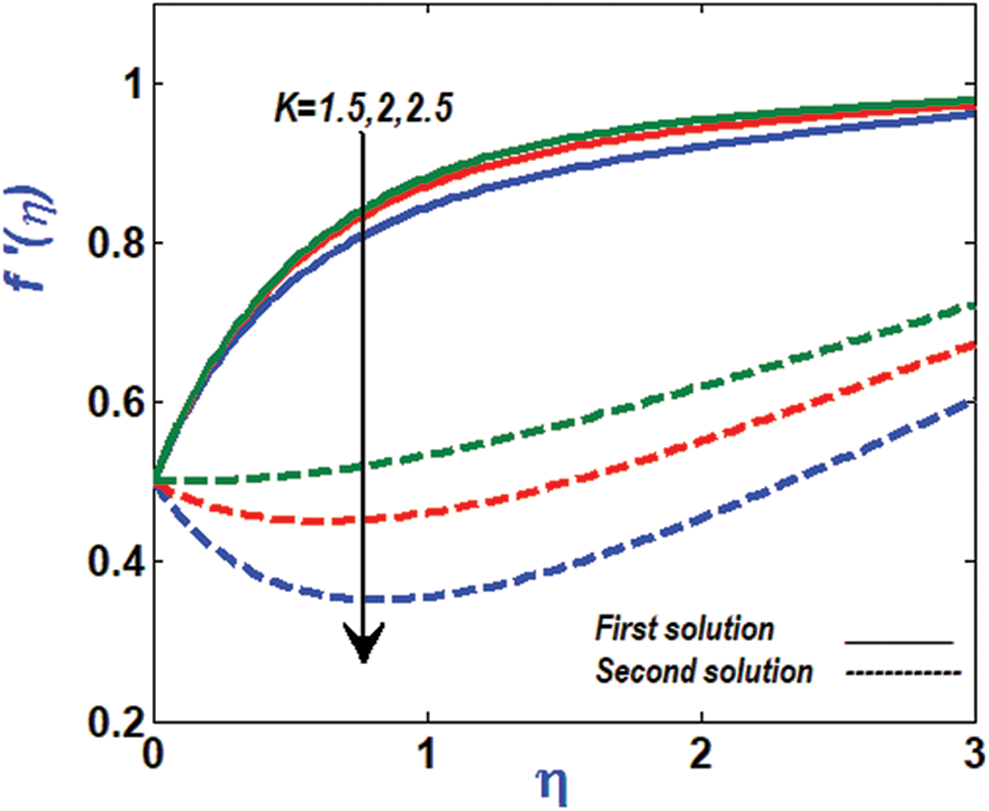
Figure 2: Variation of velocity profile against K

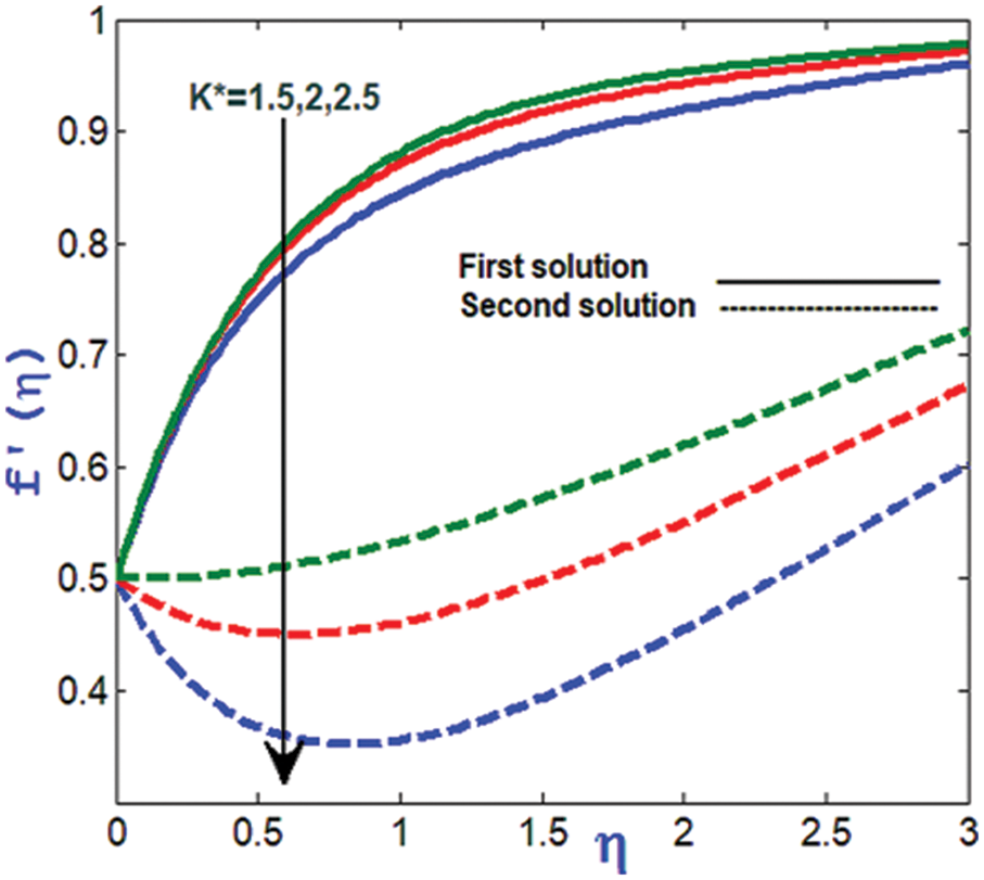
Figure 3: Variation of velocity profile against K*

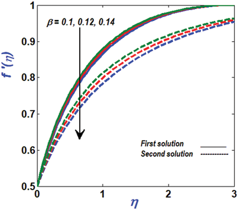
Figure 4: Variation of velocity profile against β

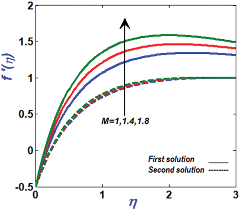
Figure 5: Variation of velocity profile against M

4.2 Micro Polar Profile

Adding higher values of the material parameter K for second solution causes the micro-rotational profile H(η) to climb sharply, as seen in Fig. 6. The first solution, on the other hand, displays the opposite tendency. This means that in the second solution, a greater amount of the material parameter yields a larger micro-rotational vector flux. Spin gradient viscosity is created by the random motion of Micropolar fluids, and this causes the profile H(η) to rise. When n=0.5 is used, the profile H(η) decreases as a function of the curvature parameter K* in Fig. 7. We can conclude that the micro-rotational flux decreases as the bent channel is curved further. In addition, because of the increased boundary layer thickness, the flow’s speed and microrotation flux will be reduced as a result of the bending. These two figures show the same profile rises for both solutions of when λ>0 is used as the channel stretch in Figs. 8 and 9. However, the profile shrinks for shrinking cases when λ<0 is used. Stretched channels had increased micro-rotational flux, therefore we can draw this conclusion.

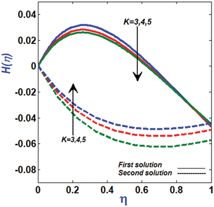
Figure 6: Variation of H(η) against K

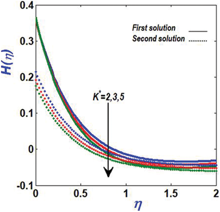
Figure 7: Variation of H(η) against K*

Figure 8: Variation of H(η) against <0

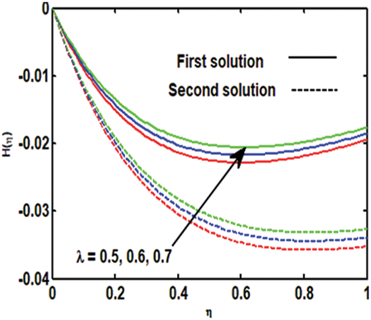
Figure 9: Variation of H(η) against λ>0

4.3 Temperature Profile

This is seen in Fig. 10, which illustrates the lower temperature profile of a bent channel. It is because we decreased the surface area with the fluid when we raised K*, and this resulted in a drop in liquid temperature. Thermophoresis aids in increasing the thermal flux in both solutions, as seen in Figs. 11 and 12. To put it another way: Large values of the parameter Nt aid in the movement of warm particles to the cooler regions of the liquid, making the liquid hotter. Furthermore, we observed that varied values of the parameter Nb have no effect on thermal activity. Fig. 13 shows that the temperature of the fluid decreases for the first solution, whereas the opposite is true for the second solution. We already know that a lower Pr number is recommended for improved energy transfer.

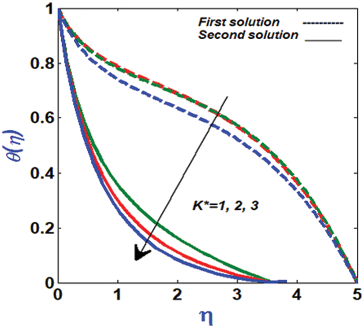
Figure 10: Variation of temperature profile against K*

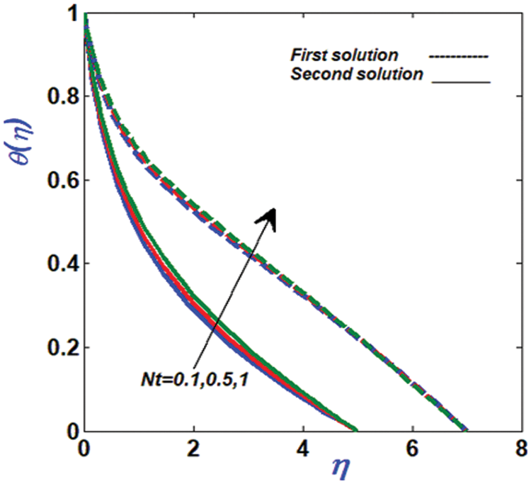
Figure 11: Variation of temperature profile against Nt

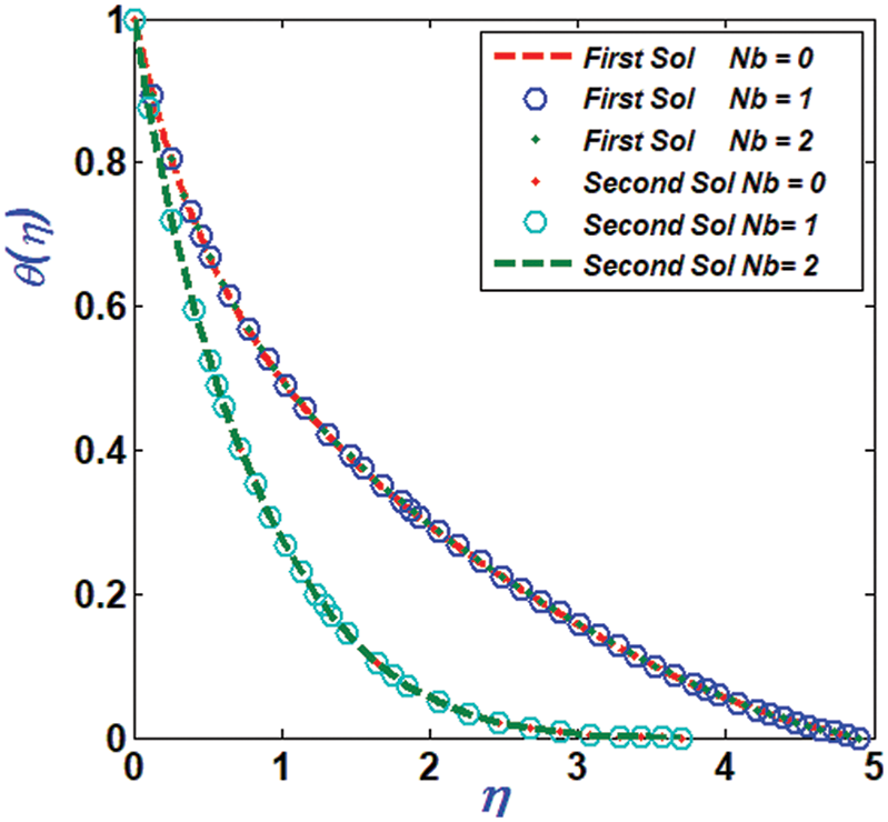
Figure 12: Variation of temperature profile against Nb

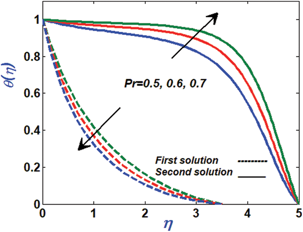
Figure 13: Variation of temperature profile against Pr

4.4 Concentration Profile

For both solutions, large values of parameter Nt cause a decrease in the concentration flux. In Fig. 14, a large quantity of parameter Nt causes the fluid to get warmer, which reduces the thickness of the concentration boundary layer. As seen in Fig. 15, both solutions benefit from the Brownian motion parameter Nb , which increases concentration flux. As we increased the parameter Nb , we saw an increase in mass transfer along the surface’s wall.

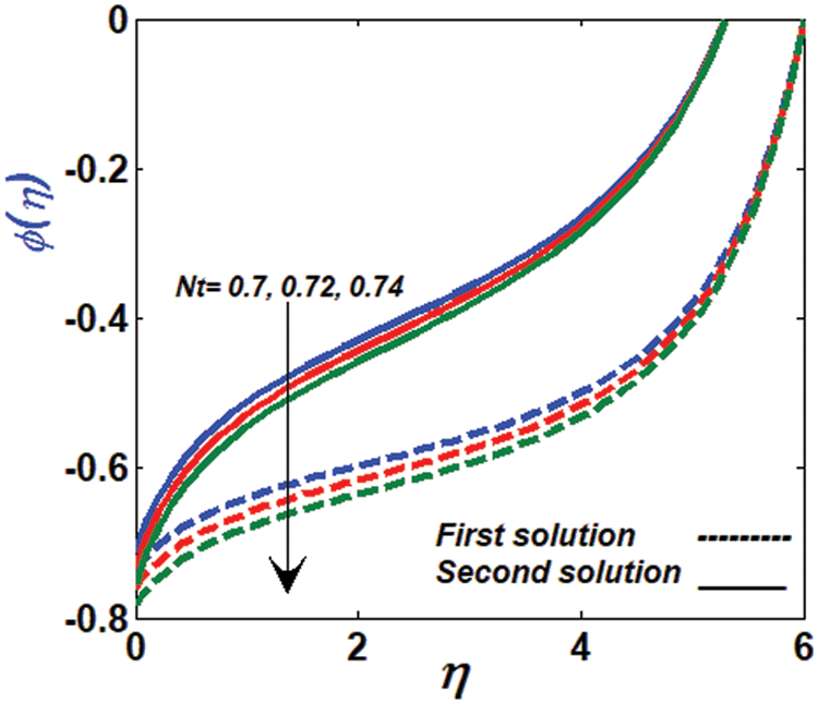
Figure 14: Variation of concentration profile against Nt

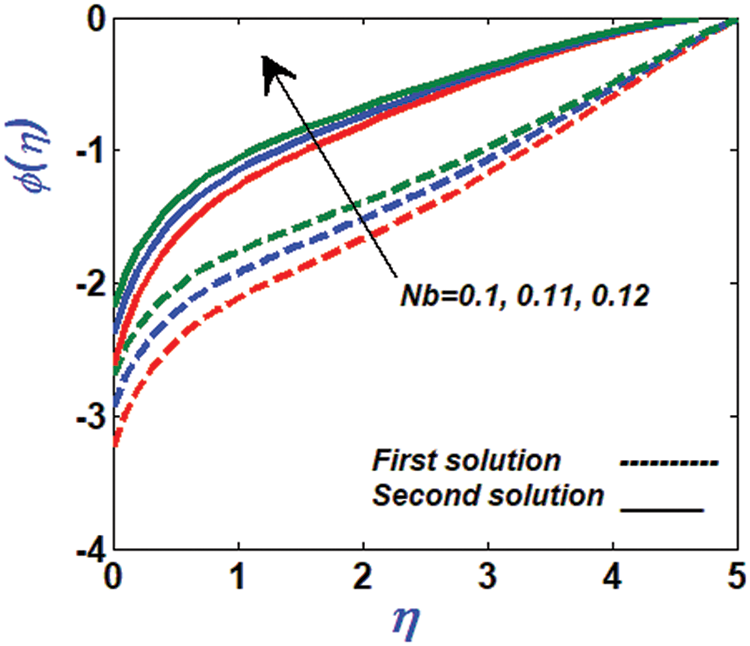
Figure 15: Variation of temperature profile against Nb

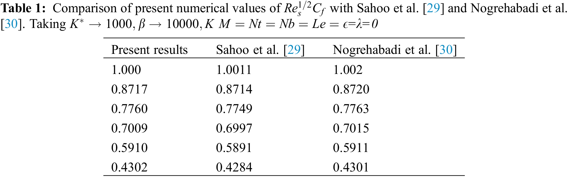
We also compare our present values of Res1/2Cf with other published results of Sahoo et al. [29] and Nogrehabadi et al. [30]. Table 1 portrays a comparison table of numerical values of Res1/2Cf when we take K∗→1000,β→10000,KM=Nt=Nb=Le=ϵ = λ =0. We conclude that our decay results are matching the values calculated in [29,30].

5  Stability Analysis

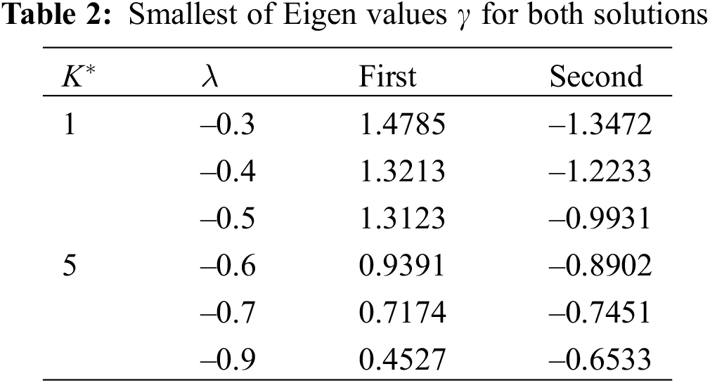
Some parametric options have been shown to have dual solutions in previous sections, as demonstrated by numerical simulations of Eqs. (9)–(13). For this reason, we used a numerical eigenvalue system of Eqs. (29)–(33) to determine the best solution. For positive lowest eigen values, we noticed that our solutions show an initial deterioration. Furthermore, we found that the solutions remained unstable when the eigen values were negative. Table 2 shows the least eigen values that were identified as a result of these solutions. Our findings show that the first options are more feasible than the second ones. According to [27,28], there were similar findings.

6  Conclusion

The performance of the Casson Micropolar nanoliquid flow mixer and energy transfer were examined in this study. We discovered that for some parametric values, our equations yield two solutions. As a result, we needed to do a stability analysis in order to select the best solution. Our steady state system was perturbed by exponential functions. Because exponential functions converge more quickly than some other function, this is why they are used. It was easy for us to identify the proper eigenvalues because they agreed so well with our possible solutions. The MATLAB solver bvp4c has stopped working.

We arrived at the following key observations:

•   We witnessed that the profile f′(η) increases if we enlarged the values of M . But the same profile is decreasing function of parameters K∗, β and K.

•   The profile H(η) is the decreasing function of parameter K∗ . However, for large values of parameter K the profile down surged in case of first and up surged for second solutions, respectively.

•   The profile θ(η) is increasing function of Nt , however it remains unchanged for different values of Nb .

•   For second solution, the function θ(η) rises high for large amounts of parameter Pr, but the profile behaves differently for other solution.

•   The profile θ(η) declines when added more values in parameter K∗ .

•   The function φ(η) declines for large values of parameter Nt , however opposite picture is portrayed by the profile when we enlarged the parameter Nb.

Acknowledgement: Authors are thanks to KFUPM for providing adequate resources for this research.

Funding Statement: The authors received no specific funding for this study.

Conflicts of Interest: The authors declare that they have no conflicts of interest to report regarding the present study.

References

 1.  Chan, W. C. W. (2020). Nano research for COVID-19. ACS Nano, 14(4), 3719–3720. DOI 10.1021/acsnano.0c02540. [Google Scholar] [CrossRef]

 2.  Yoo, D. H., Hong, K. S., Yang, H. S. (2007). Study of thermal conductivity of nanofluids for the application of heat transfer fluids. Thermochimica Acta, 455(1–2), 66–69. DOI 10.1016/j.tca.2006.12.006. [Google Scholar] [CrossRef]

 3.  Fetecau, C., Vieru, D., Azhar, W. A. (2017). Natural convection flow of fractional nanofluids over an isothermal vertical plate with thermal radiation. Applied Sciences, 7(3), 247. DOI 10.3390/app7030247. [Google Scholar] [CrossRef]

 4.  Khan, N. S., Gul, T., Islam, S., Khan, I., Alqahtani, A. M. et al. (2017). Magnetohydrodynamic nanoliquid thin film sprayed on a stretching cylinder with heat transfer. Applied Sciences, 7(3), 271. DOI 10.3390/app7030271. [Google Scholar] [CrossRef]

 5.  Mekheimer, K. S., Ramadan, S. F. (2020). New insight into gyrotactic microorganisms for bio-thermal convection of Prandtl nanofluid over a stretching/shrinking permeable sheet. SN Applied Sciences, 2(3), 1–11. DOI 10.1007/s42452-020-2105-9. [Google Scholar] [CrossRef]

 6.  Ahmad, S., Nadeem, S., Muhammad, N., Issakhov, A. (2020). Radiative SWCNT and MWCNT nanofluid flow of Falkner-Skan problem with double stratification. Physica A: Statistical Mechanics and its Applications, 547, 124054. DOI 10.1016/j.physa.2019.124054. [Google Scholar] [CrossRef]

 7.  Akram, J., Akbar, N., Tripathi, D. (2020). Comparative study on ethylene glycol-based Ag-Al2O3 and Al2O3 nanofluids flow driven by electroosmotic and peristaltic pumping. Physica Scripta, 95(11), 115208. DOI 10.1088/1402-4896/abbd6b. [Google Scholar] [CrossRef]

 8.  Wahid, N. S., Arifin, N. M., Khashie, N. S., Pop, I. (2021). Hybrid nanofluid slip flow over an exponentially stretching/shrinking permeable sheet with heat generation. Mathematics, 9(1), 30. DOI 10.3390/math9010030. [Google Scholar] [CrossRef]

 9.  Haider, F., Hayat, T., Alsaedi, A. (2021). Flow of hybrid nanofluid through Darcy-Forchheimer porous space with variable characteristics. Alexandria Engineering Journal, 60(3), 3047–3056. DOI 10.1016/j.aej.2021.01.021. [Google Scholar] [CrossRef]

10. Abbas, N., Nadeem, S., Saleem, A., Malik, M. Y., Issakhov, A. et al. (2021). Models base study of inclined MHD of hybrid nanofluid flow over nonlinear stretching cylinder. Chinese Journal of Physics, 69(4), 109–117. DOI 10.1016/j.cjph.2020.11.019. [Google Scholar] [CrossRef]

11. Eringen, A. C. (1966). Theory of micropolar fluids. Journal of Mathematics and Mechanics, 16(1), 1–18. DOI 10.1512/iumj.1967.16.16001. [Google Scholar] [CrossRef]

12. Willson, A. J. (1970). Boundary layers in micropolar liquids. Mathematical Proceedings of the Cambridge Philosophical Society, 67(2), 469–476. DOI 10.1017/S0305004100045746. [Google Scholar] [CrossRef]

13. Asghar, Z., Ali, N., Sajid, M. (2017). Interaction of gliding motion of bacteria with rheological properties of the slime. Mathematical Biosciences, 290, 31–40. DOI 10.1016/j.mbs.2017.05.009. [Google Scholar] [CrossRef]

14. Abbas, N., Nadeem, S., Malik, M. Y. (2019). On extended version of Yamada-Ota and Xue models in micropolar fluid flow under the region of stagnation point. Physica A: Statistical Mechanics and its Applications, 542(1), 123512. DOI 10.1016/j.physa.2019.123512. [Google Scholar] [CrossRef]

15. Ismail, H. N. A., Abourabia, A. M., Hammad, D. A., Ahmed, N. A., El Desouky, A. A. (2020). On the MHD flow and heat transfer of a micropolar fluid in a rectangular duct under the effects of the induced magnetic field and slip boundary conditions. SN Applied Sciences, 2(1), 1–10. DOI 10.1007/s42452-019-1615-9. [Google Scholar] [CrossRef]

16. Abbas, N.,Nadeem, S., Khan, M. N. (2021). Numerical analysis of unsteady magnetized micropolar fluid flow over a curved surface. Journal of Thermal Analysis and Calorimetry, 147,6449–6459. DOI 10.1007/s10973-021-10913-0. [Google Scholar] [CrossRef]

17. Raza, A., Haq, R. U., Shah, S., Alansari, M. (2022). Existence of dual solution for micro-polar fluid flow with convective boundary layer in the presence of thermal radiation and suction/injection effects. International Communication in Heat and Mass Transfer, 131(1), 105785. DOI 10.1016/j.icheatmasstransfer.2021.105785. [Google Scholar] [CrossRef]

18. Casson, N. (1959). A flow equation for pigment-oil suspensions of the printing ink type, pp. 84–104. New York, Oxford: Pergamon: Rheology of Disperse Systems. [Google Scholar]

19. McDonald, D. A. (1974). Blood flows in arteries, 2nd ed. London. DOI 10.1113/expphysiol.1975.sp002291. [Google Scholar] [CrossRef]

20. Nadeem, S., Mehmood, R., Akbar, N. S. (2014). Optimized analytical solution for oblique flow of a Casson-nano fluid with convective boundary conditions. International Journal of Thermal Sciences, 78, 90–100. DOI 10.1016/j.ijthermalsci.2013.12.001. [Google Scholar] [CrossRef]

21. Nadeem, S., Haq, R. U., Akbar, N. S. (2014). MHD three-dimensional boundary layer flow of Casson nanofluid past a linearly stretching sheet with convective boundary condition. IEEE Transactions on Nanotechnology, 13(1), 109–115. DOI 10.1109/TNANO.2013.2293735. [Google Scholar] [CrossRef]

22. Mustafa, M., Khan, J. A. (2015). Model for flow of Casson nanofluid past a non-linearly stretching sheet considering magnetic field effects. AIP Advances, 5(7), 077148. DOI 10.1063/1.4927449. [Google Scholar] [CrossRef]

23. Sarkar, S., Endalew, M. F. (2019). Effects of melting process on the hydromagnetic wedge flow of a Casson nanofluid in a porous medium. Boundary Value Problems, 43, 1–14. DOI 10.1186/s13661-019-1157-5. [Google Scholar] [CrossRef]

24. Ibrar, N., Reddy, M. G., Shehzad, S. A., Sreenivasulu, P., Poornima, T. (2020). Interaction of single and multi-walls carbon nanotubes in magnetized-nano Casson fluid over radiated horizontal needle. SN Applied Sciences, 2(4), 1–12. DOI 10.1007/s42452-020-2523-8. [Google Scholar] [CrossRef]

25. Nayak, M. K., Prakash, J., Tripathi, D., Pandey, V. S., Shaw, S. et al. (2020). 3D Bioconvective multiple slip flow of chemically reactive Casson nanofluid with gyrotactic micro-organisms. Heat Transfer, 49(1), 135–153. [Google Scholar]

26. Khan, M. R., Elkotb, M. A., Matoog, R. T., Alshehri, N. A., Mostafa A. H. et al. (2021). Thermal features and heat transfer enhancement of a Casson fluid across a porous stretching/shrinking sheet: analysis of dual solutions. Case Studies in Thermal Engineering, 28(4), 101594. DOI 10.1016/j.csite.2021.101594. [Google Scholar] [CrossRef]

27. Weidman, P. D., Kubitschck, D. G. (2006). The effect of transpiration on self-similar boundary layer flow over moving surfaces. Science Direct, 44(11–12), 730–737. DOI 10.1016/j.ijengsci.2006.04.005. [Google Scholar] [CrossRef]

28. Rosca, N. C., Pop, I. (2015). Unsteady boundary layer flow over a permeable curved/shrinking surface. European Journal of Mechanics-B/Fluids, 51, 61–67. DOI 10.1016/j.euromechflu.2015.01.001. [Google Scholar] [CrossRef]

29. Sahoo, B., Poncet, S. (2011). Flow and heat transfer of a third-grade fluid past an exponentially stretching sheet with partial slip boundary condition. International Journal of Heat and Mass Transfer, 54(23–24), 5010–5019. DOI 10.1016/j.ijheatmasstransfer.2011.07.015. [Google Scholar] [CrossRef]

30. Noghrehabadi, A., Pourrajab, R., Ghalambaz, M. (2012). Effect of partial slip boundary condition on the flow and heat transfer of nanofluids past stretching sheet prescribed constant wall temperature. International Journal of Thermal Sciences, 54(1), 253–261. DOI 10.1016/j.ijthermalsci.2011.11.017. [Google Scholar] [CrossRef]