A CFD Model to Evaluate Near-Surface Oil Spill from a Broken Loading Pipe in Shallow Coastal Waters

1  Introduction

Oil transportation via pipelines is the most common method of moving oil from one location to another. There is a risk of oil spills occurring whether these oil pipelines are located underwater, on land, or along the water surface via oil jetty pipelines. Water surface oil spills are often observed and reported to occur as a result of accidents, collisions, or leakages of various types of marine oil vessels and rarely by broken pipelines at the water surface; therefore, it is important to note that water surface oil spills caused by the former involve the direct release and spread of the oil on the sea surface. The type of oil and the ambient seawater conditions generally determine the extent of the oil spreading and its subsequent behavior. When oil spills on the sea surface, it spreads and forms a thin layer of oil slick [1,2]. This oil slick is then subjected to several natural processes that alter its properties, dictating its behavior in the environment. These processes are referred to collectively as the oil weathering processes. The majority of water surface oil spill models in use today were created to simulate these weathering processes using empirical equations based primarily on experimental data [3–8].

However, this investigation involved a water surface oil spill in the form of a jet flow, caused by a broken jetty pipeline that released heavy oil beneath the water surface. The heavy oil became trapped at a shallow water depth, and then travelled horizontally for a substantial distance in the direction of the ambient current. The majority of existing literature investigates the movement of oil underwater due to water surface spills as oil droplets in water rather than as an oil plume. This oil flow movement in the water column is commonly referred to as dispersion [9–12]. The goal of this research is to use computational fluid dynamics to determine what caused the oil plume studied herein to become suspended or achieve neutral buoyancy in the water column.

2  The Research Problem

On December 17th, 2013, an oil spill at the Trinidad and Tobago state-owned oil company refinery (PETROTRIN) in Pointe-a-Pierre injected over 7000 barrels of heavy bunker C fuel oil beneath the sea surface in the Gulf of Paria, for just over three hours. Fig. 1a through to Fig. 1d, respectively depicts the location of Trinidad and Tobago in relation to South America. The island of Trinidad is bordered on the east by the Atlantic Ocean, on the north by the Caribbean Sea and by the Columbus Channel on the south. To the west, Trinidad’s west coast is separated from mainland Venezuela by the Gulf of Paria. The Gulf of Paria is a semi-enclosed sea with a net flow from south to north. The Gulf of Paria is located on the west coast of Trinidad and the spill site is located south-west of Trinidad in the Pointe-a-Pierre area, and a satellite imagery of the oil refinery, which is the source of the spilled oil is shown, respectively. Fig. 2 which was extracted from the EU Copernicus Marine Environment and Monitoring Service (CMEMS) web portal, depicts the salinity of the sea surface layer and the sea surface temperature of the Gulf of Paria, respectively.

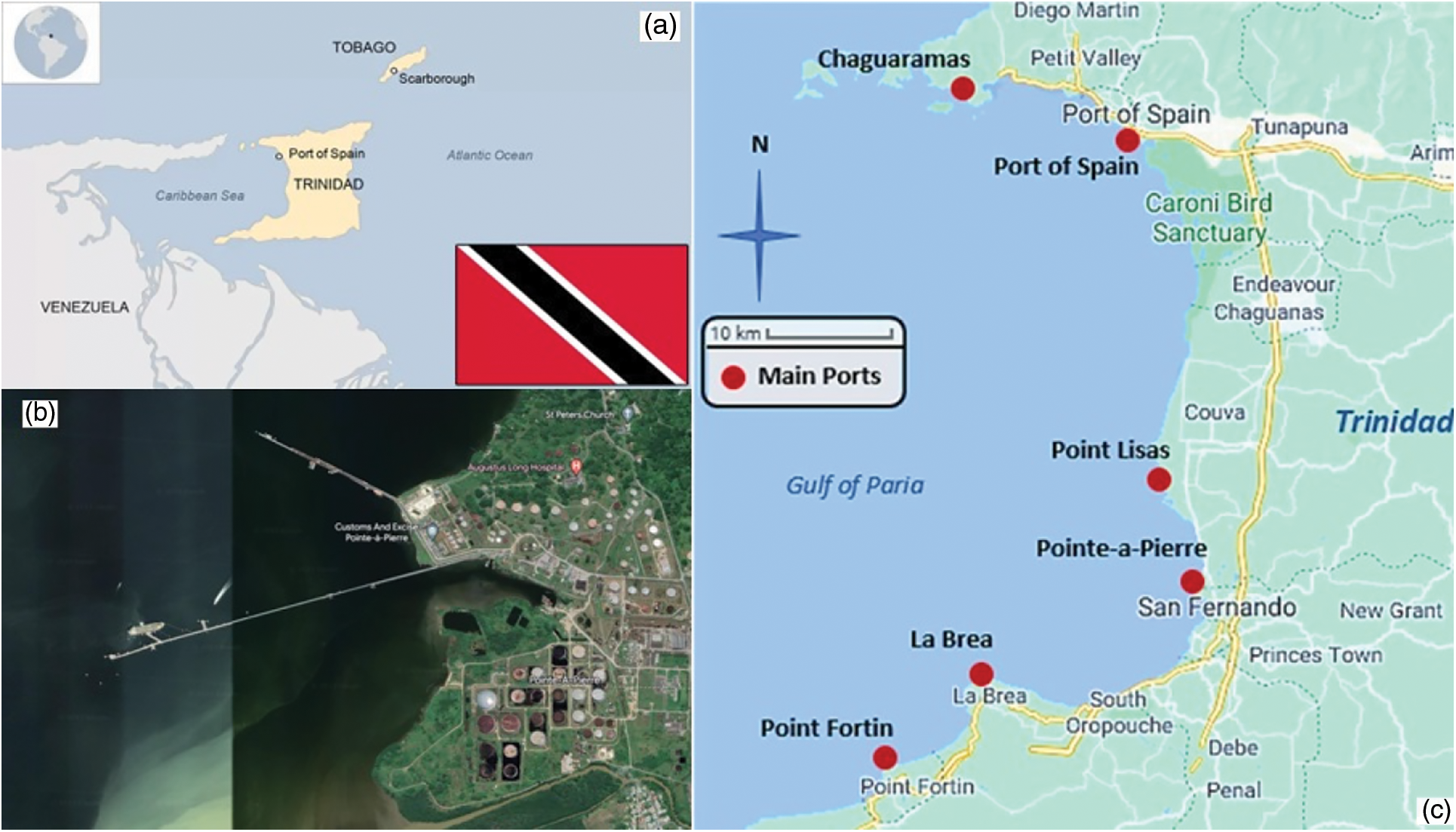
Figure 1: (a) Trinidad and Tobago in relation to South America (b) Gulf of Paria & Pointe-a-Pierre (c) Petrotrin refinery

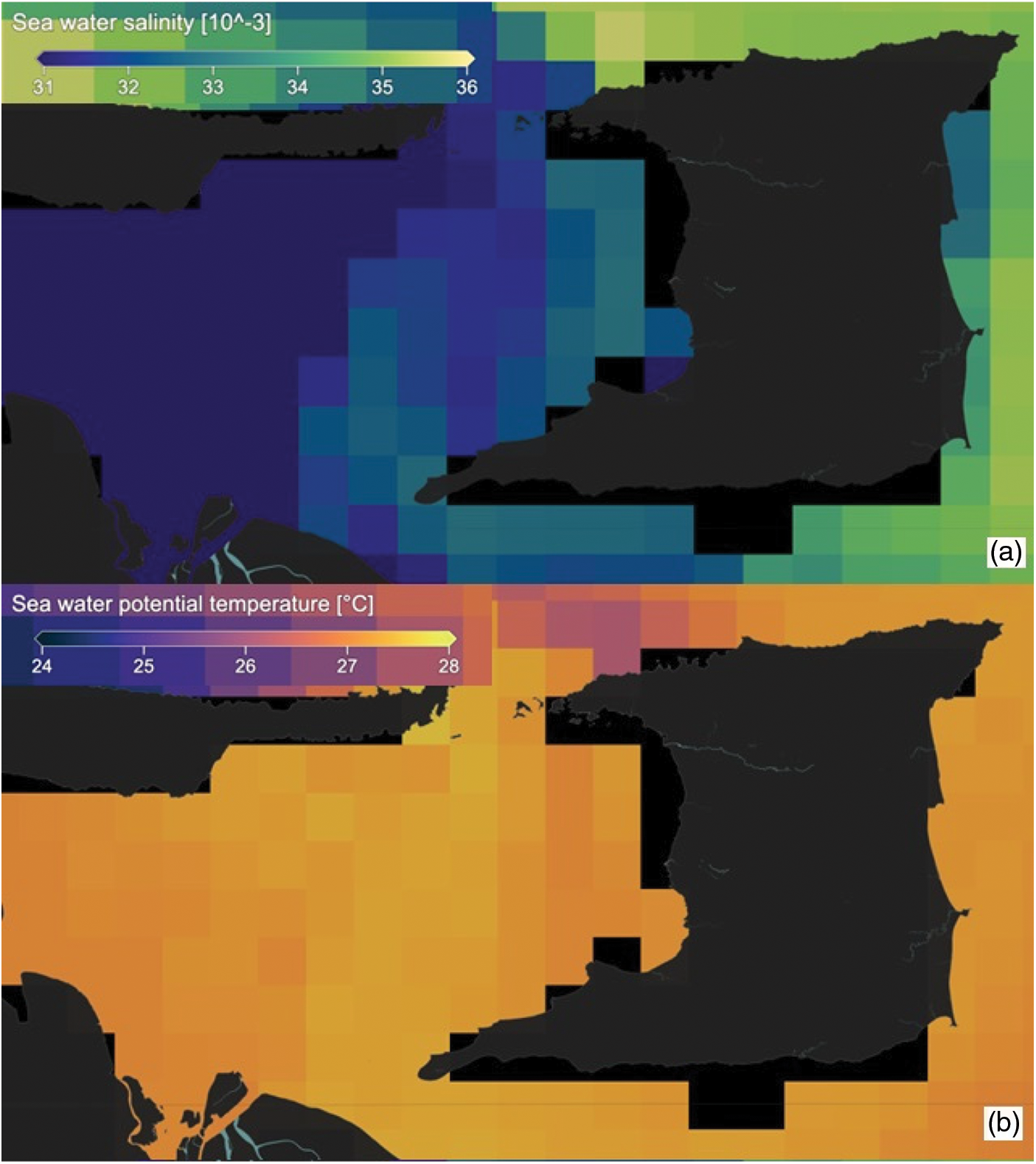
Figure 2: Satellite observations (a) salinity of the sea surface (b) sea surface temperature

The cause of this incident was due to an acutely angled broken surface loading pipeline issuing heavy oil into the shallow near-shore coastal waters. The spilled oil from the broken pipeline almost immediately sank to a depth of about 2–5 m below the water’s surface and travelled horizontally, in the direction of the ambient current, until it resurfaced as a heavy oil slick approximately 3.5 km from the spill site. Following the event, only a slight sheen was observed near the spill site. This seemingly unexpected oil behavior drew a lot of local media and academic attention, and it sparked a lot of debate. The first problem was that there was no visible oil slick on the surface of the water where the leak initially began, and the quantity of sheen observed was insufficient to account for the volume of oil released. Another reason for concern was that it was expected that the oil that was deposited on the water surface would remain on the surface, generating a surface oil slick. This surface oil slick would then go through a variety of weathering processes that would change the oil over the course of time. However, this did not occur, instead the discharged oil spent no significant residence time on the water surface but was immediately pushed beneath the water surface. This oil flow behaviour is rarely observed and studied. According to the literature, the major possible mechanisms that would allow oil to sink are the density of the oil, the attachment of dispersed oil droplets to suspended sediments in the water column, and weathering processes of oil such as evaporation or dissolution of lighter oil components that can reduce the buoyancy of oil resulting in a denser oil with the potential to sink [13–17]. Fig. 3 shows the location of the spill site in relation to the Gulf of Paria.

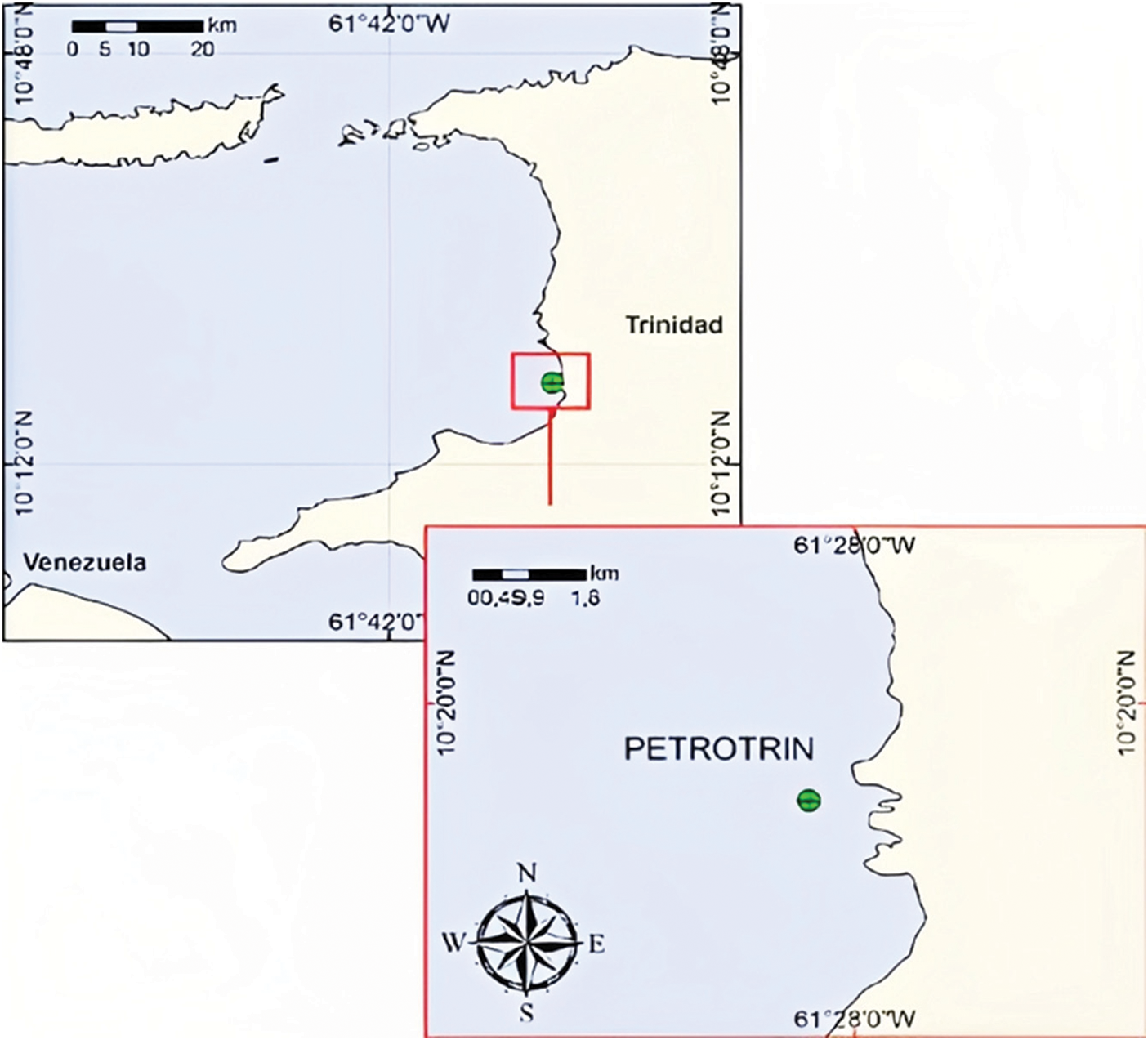
Figure 3: Study area at the Gulf of Paria, with the location of the spill site (taken from an unpublished emergency oil spill modelling in the Gulf of Paria, Trinidad report, January, 2014)

This oil plume behavior will then become more concerning, as it was argued where the majority of the oil went and what mechanism would allow the oil to be suspended and moved horizontally in the water column, especially since the oil is heavy fuel oil that is expected to sink to the sea floor. A local investigation report (which is not made available in the public domain) on the said oil spill, stated that an aerial survey was conducted and it was observed that “a long, narrow patch of oil appeared to be trapped within the water column and hence under the surface of the water”. This research paper focuses on the mechanism enabling neutral buoyancy of the oil [18–20], that is, the horizontal movement and suspended entrapment of the oil. Fig. 4 depicts a schematic of the oil flow behaviour as it moves from near-field jet-like behaviour to an oil plume in the intermediate or transport field, and finally to the far-field, where the oil resurfaced, possibly due to the oil encountering a much shallower water depth (shoaling). The research is concerned with oil flow behaviour in the intermediate or transport field as shown in Fig. 4.

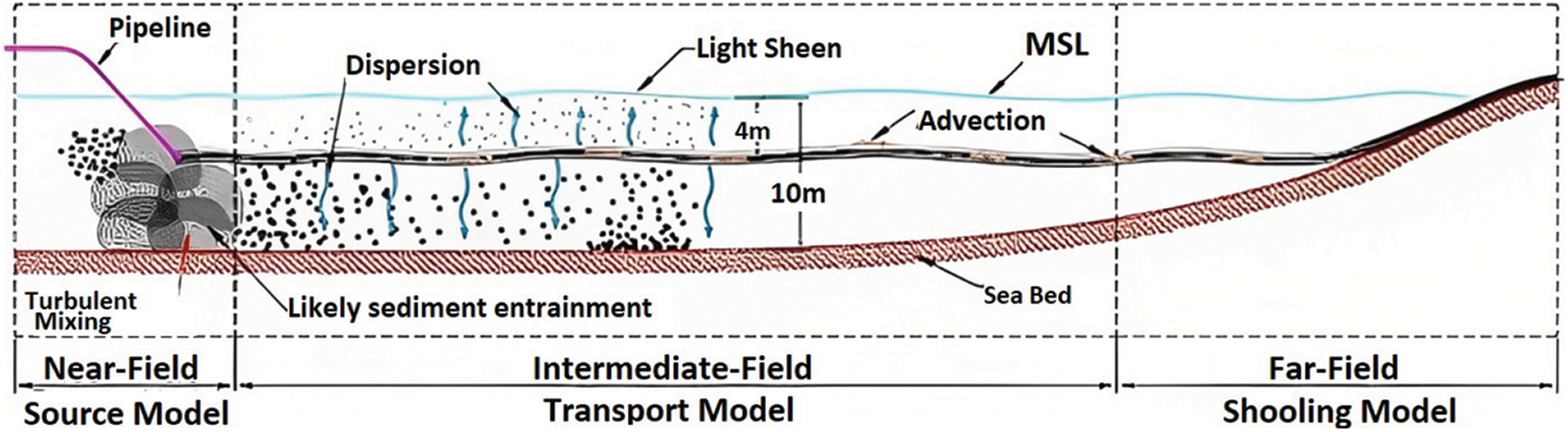
Figure 4: Schematic of profile of the oil behavior in the intermediate field

This study has the potential to provide insight and aid in informing cleanup decisions in situations where oil discharged from a broken surface pipeline may exhibit unusual behavior in the water column, such as submergence and neutral buoyancy.

Much of the literature explains the vertical subsurface movement of oil from a surface spill using mathematical models based on a set of empirical techniques [2,3,12,15,21–24]. Oil spill models that track oil transport and particle dispersion in the water column are also commercially available [1,2,10,25–27]. According to [3], advection of suspended oil refers to the movement of oil droplets that have become entrained in the water column and are being propelled by the water current, and all of these models allow for vertical subsurface entrainment and transport of oil. These models, however, pay little to no attention to the horizontal advection motion of a plume-like oil mass suspended beneath the water surface, whose advective movement is dictated by the movement of the water body and whose suspension beneath the water surface is due to entrapment in a sensitive temperature pycnocline within the water column. The Delvigne and Sweeney technique, which calculates the entrained oil mass per unit area and unit time, is now used by most models to investigate oil dispersion in the water column. This proposed expression is summarized in Eq. (1) as follows:

∂Q∂d|d0=C0Dba0.57ScovFwcd00.7 (1)

where:

C0 = Oil dispersion parameter related to oil viscosity

d0 = Oil droplet diameter

Q = Entrainment rate of oil droplets per unit surface area

Scov = Fraction of sea surface covered by oil and

Fwc = Fraction of the sea surface hit by breaking waves per unit time

Dba0.57  = Dissipation energy of the wave

Integrating the gradient of the dispersion rate over all droplet classes from (dmax) till (dmin) gives the total entrainment rate Q of the oil per square meter (Eq. (2)):

Q=∫dmindmax∂Q∂d|d0dd0=dmax1.71.7C0Dba0.57FwcScov (2)

This current methodology for oil penetrating the water surface from the transformation of a floating surface oil slick into oil droplets has been implemented and improved numerically and analytically in numerous ways by several authors [28–30]. Despite the fact that these models continue to give progressively satisfying findings, the dynamics of heavy fuel oil discharging into the underlying water surface owing to an injection source and transitioning into an underwater plume are not sufficiently studied, as this necessitates the consideration that the very high viscosity nature of heavy bunker C fuel can resist the breaking up of oil being dispersed as droplets in the water column [31], and hence this work approaches the problem initially in a very basic manner using computational fluid dynamics to solve an underwater oil plume flow.

3  Mathematical Model

For the purpose of determining the movement of the spilled oil through the water column, the mathematical formulation closely follows the two-dimensional incompressible Navier-Stokes momentum equations, as well as the continuity and energy equations. Although the flow can be considered a two-phase flow, for the sake of simplicity, the interaction of oil and water is not taken into account, instead the oil is considered to be carried by the movement of the ambient water, which is somewhat akin to core-annular flow in a horizontal pipe in terms of the buoyancy of the heavy viscous oil core on the water as the water transports the oil through the pipe [32–34] and so Newtonian behavior can be assumed [35]. Also, the heavy oil flow in seawater herein, is assumed to be in the laminar flow regime as well as the ambient seawater flow field, and hence a computational fluid dynamics approach of the single-phase flow equations is applicable. This assumption is valid, as the problem is simplified by assuming since heavy bunker C fuel oil is commonly characterized as having very high viscosity [36–38], therefore, implying a low Reynolds number and hence further assuming turbulence conditions are never reached [39]. In Cartesian form, these equations (Eq. (3) through Eq. (6)) may be represented correspondingly as:

Continuity equation (Conservation of mass)

∂u∂x+∂w∂z=0 (3)

The x-momentum equation

ρ0(∂u∂t+u∂u∂x+w∂u∂z)−μ∇2u+∂p∂x=0 (4)

The z-momentum equation

ρ0(∂w∂t+u∂w∂x+w∂w∂z)−μ∇2w+∂p∂z=ρ′g (5)

The energy equation

∂SG∂t+u∂SG∂x+w∂SG∂z=D(∂2SG∂x2+∂2SG∂z2) (6)

In the equations, t represents time, x and z represent the horizontal and vertical coordinates, while u and w represent the horizontal and vertical velocity components, respectively. The specific gravity ( SG ) of the input fluid is defined as the ratio of the density of a substance to the density of a reference substance. The diffusivity coefficient is represented by D; p represents the pressure; ρ′ is the deviation density; g represents the gravitational acceleration; μ is the dynamic viscosity. ρ0 stands for the density of the fluid that is present in the environment.

Note that in the equation for energy, the specific gravity notation SG was substituted for the temperature T. Given that specific gravity is a ratio of densities (as stated above), and that if the density value at the denominator is known, the density at the numerator can be solved as a function of temperature, the mathematical justification for this statement is as follows: specific gravity is a function of temperature, sometimes known as SG = f(T). Using the equation of state ρ=f(T, SG) and assuming for the sake of a first approximation that the computational domain is homogeneous (has a constant salinity), i.e., ρ0 = 1, the following is what we get:

SG=ρ(T)ρ0 (7)

where ρ0 is known.

ρ(T)=ρ0∗[1−α(T−T0)]⇒SG=1−α(T−T0)⇒T=T0+1−SGα (8)

Therefore, the differential energy equation is the same, as T is linear in SG and so SG is used instead of T.

In this formulation, the following dimensionless variables are utilized, where U denotes the reference velocity for the fluid system moving in the horizontal direction:

x∗=xL (9)

z∗=zL (10)

t∗=tLU (11)

p∗=pρoU2 (12)

u∗=uU (13)

w∗=wU (14)

The solution to Eq. (4) may be found by inserting the dimensionless variables in place of the *:

∂u∂t+u∂u∂x+w∂u∂z=−∂p∂x+1Re(∂2u∂x2+∂2u∂z2) (15)

where Re is the dimensionless Reynolds number, which is considered in this case as the ratio of the Peclet number, Pe=fluid speed, u∗horizontal distance, LD to the Prandtl number Pr=momentum viscosity(kinematic viscosity), υthermal diffusivity, α .

It is therefore given as:

Re=uLυ (16)

Similarly, Eq. (5) in non-dimensionalize form becomes:

∂w∂t+u∂w∂x+w∂w∂z−1Re∇2w+1ρ0∂p∂z=−g′ρ′ρ0 (17)

The buoyancy force term in Eq. (9) is:

fB=g′ρ′ρ0 (18)

As a result, it is more practical to allow the buoyancy force term be equal to RiT, which may be written as:

fB=ρ′g′ρ0=RiT (19)

In this equation, Ri is the dimensionless Richardson number, which is defined as the ratio of the buoyancy term to the flow shear term. The following is the Richardson number in full:

Ri=accleration due to gravity,  g∗horizontal distance,  hfluid's speed,  u2

Both the continuity equation and the transport equation may be solved by employing the same non-dimensional method. As a result, using the non-dimensionalization and simplification strategy that was described before, we were able to construct and numerically solve the following set of equations (Eq. (20) through Eq. (23)):

∂u∂x+∂w∂z=0 (20)

∂u∂t+u∂u∂x+u∂w∂z=−∂p∂x+1Re(∂2u∂x2)+1Re(∂2u∂z2) (21)

∂w∂t=u∂w∂x+w∂w∂z=−∂p∂z+1Re(∂2w∂x2)+1Re(∂2w∂z2)+RaPrT (22)

∂SG∂t+u∂SG∂x+w∂SG∂z=∂2SG∂x2+∂2SG∂z2 (23)

where Ra is the Raleigh number which describes the ratio of buoyancy and viscous forces and this is multiplied by the Prandtl number, which is the ratio of the momentum and thermal diffusivityacting on the flow. Therefore, the buoyancy term due to convection is expressed as the Raleigh number times the Prandtl number times:

T:Bμ×υα=RaPrT (24)

Eq. (20) through to Eq. (23) are then solved numerically by the finite difference Projection method approximations. Details of this numerical analysis are explained in the following section.

4  Numerical Technique

In order to solve the set of governing Eq. (21) through (13), the Chorin-type projection approach, which is described in [40,41], is utilized. The strategy for finding a solution using the Projection method is a two-stage process that involves a scheme containing a pressure corrector step and a predictor step, respectively. The momentum equations are used to compute an intermediate velocity field in the first step. In spite of this, the continuity equation is not satisfied by this velocity; hence, the second step entails solving a Poisson equation for the pressure, which is determined from the continuity equation. A divergence-free velocity field is created by projecting an intermediate velocity field onto it using the pressure that was determined. The following is a very brief summary of the steps needed to be taken in order to solve the governing equations, exhibiting the important equations:

Step 1. We begin with the predictor step in which an incomplete form of the momentum equations is integrated to yield an approximate velocity field, which will not be divergence free. That is to say, the system is advancing in time to find an intermediate flow field U* and W* using explicit Euler that satisfies the non-linear advection and diffusion terms as follows:

U∗−UnΔt=−((Un)2)x−(UnWn)z+1Re(Uxx∗∗+Uzz∗∗) (25)

W∗−WnΔt=−(UnWn)x−((Wu)2)z+1Re(Wxx∗∗+Wzz∗∗) (26)

Step 2. The pressure corrector step now includes the addition of a projection operator, also known as a pressure term, in order to make the necessary adjustments to the continuity equation, also known as the process of solving a Poisson equation:

−Δpn+1=−1Δt∇U∗ (27)

Computing the gradient of the pressure and the velocity field at time step n + 1 gives:

Un+1=U∗−Δt∇pn+1 (28)

In a manner analogous to this, the energy equation was solved using this method. These stages are repeated in an iterative manner until the solution is converged, at which point the integration moves on to the following phase.

4.1 Spatial Discretization

The process of spatial discretization is carried out on a grid that has been shifted, with the pressure p positioned in the center of each cell, and the velocities U and W located at the midway points of the vertical and horizontal cell boundaries, respectively. This allows for the grid to be broken up into a series of alternating rows and columns. Fig. 5 is an illustration of an example of the staggered grid-approach structure that is utilized in the process of describing the physical quantities that are at play in the situation.

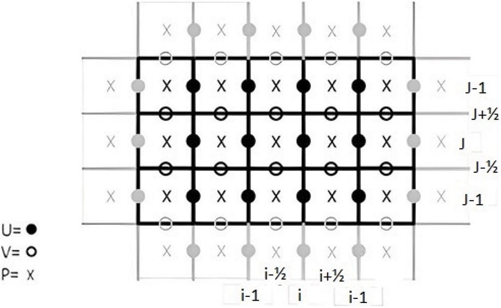
Figure 5: Grid with staggered cells that demonstrates the spatial discretization

The domain boundary is shown by the thick black line in Fig. 5, which also serves as the surface onto which the boundary conditions are enforced. The points that are dark are considered to be interior points, the points that are grey and located on the border are considered to be boundary points, and the points that are located outside of the domain are considered to be dummy or bluff points.

Only the unknown velocity values at the inner cells are included in the matrices U and W that represent velocity; the known boundary values are not included. When time equals zero (t = 0), all of the velocities is set to zero initially, indicating that the fluid is in a state of complete stillness. A major contrast is made between the inner points and the discretization of first order derivatives. The results include the boundary points in U and W in the matrices, the matrices are expanded at the right, left, top, and bottom bounds. The following is an illustration of the definition of the central differences for the inner horizontal u and vertical w velocity points:

u=ui+12j−ui−12jh (29)

and

w=wi,j+12−wi,j−12h (30)

This is not the case for advection (non-linear) components, which are computed using velocity field values on the control volume borders that differ from the sites where the discrete velocity field is specified. The grid discretization is enough for this relatively basic oil flow case, which is a first step before expanding the issue to account the further intricacies of the oil flow behavior.

4.2 Boundary Conditions

The following constitutes the boundary conditions: The Dirichlet boundary condition requires a value to be specified at the boundary; hence, the horizontal velocity component U on the left and right borders of the computational domain must be directly applied because the velocity points in question are located on those boundaries. On both the top and bottom limits, the vertical velocity W is subject to the identical conditions that must be satisfied. On the other hand, the following is how the boundary conditions are enforced for U on the top and bottom bounds and W on the left and right boundaries:

Ub=Uin+Uout2 (31)

Uin=Ub−Uout=2Ub (32)

The Neumann boundary condition specifies the normal derivative value at the boundary point. The Neumann boundary condition specifies a zero value for the normal derivative along the boundary, which is used as follows:

Ub−Uinh=0 (33)

and for the pressure: ∂p∂n=0.

This configuration makes it possible for the oil to travel both vertically and horizontally, as well as to be suspended at a level below the water surface. Take note that the symbol for specific gravity is ρ in Fig. 6.

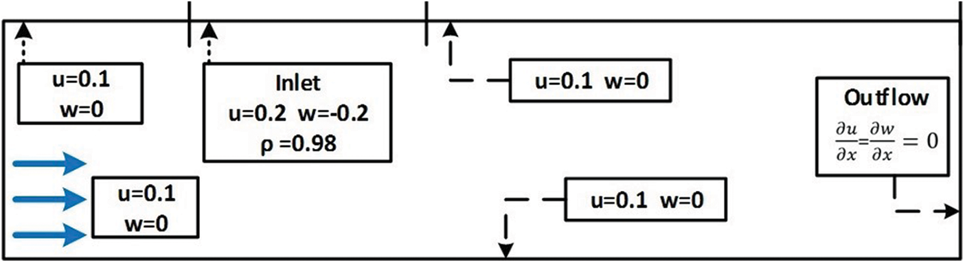
Figure 6: Problem geometry indicating the flow problem and various boundary conditions

5  Results and Discussion

5.1 The Model Setup

In this approach, the focus of the research is on the intermediate field, which is the field where the oil was seen at a shallow depth of (<10 m) and travelling horizontally. The gravity of oil, as determined by the American Petroleum Institute (API), which is a measurement of how light or heavy oil is in comparison to water. Any oil that has an API gravity value that is lower than 10 will be heavier than water, whereas any oil that has an API gravity value that is higher than 10 will be less dense than water. In this case, the discharged heavy bunker C fuel oil is said to have an API value of 13.6 and according to the oil weight classification by [42]. Oil with API less than 22.3 is considered heavy oil. This aspect draws attention to the significance of the research problem, where the oil is a heavy oil with API above 10. This feature of the oil having the capacity to float as well as being able to sink, as it is considered a heavy oil, draws attention to the significance of the research challenge, and by extension, the movement of oil through the water column. Further, the specific gravity of the oil, SG which is given as: SG = 141.5/API + 131.5, is calculated to be 0.98, and according to [43], the specific gravity of heavy N0.6 fuel oil can vary from 0.95 to greater than 1.03, thus, such spilled oil can float, suspend in the water column or sink. Hence, we see, in this case, the oil becomes suspended in the water column.

It is more practical to examine the behavior of the oil travelling at a relatively shorter horizontal distance in order to reduce the amount of computing expenditure and complexity involved. The input oil density was estimated to be 0.98 times the predicted specific gravity (SG) as a first approximation. The horizontal ambient velocity of 0.1 m/s and an oil exit velocity of 0.2 m/s were used. According to what is seen in Fig. 7a, the zonal east-west velocity of the ambient receiving environment is on the same order of magnitude as about 0.1 m/s. A regular rectangular grid with dimensions of 10 meters in the vertical z direction and 40 meters in the horizontal x direction makes up the computational grid. Additionally, the mesh size in both directions is set to 100 × 100. The entire amount of time that the model was run for was equal to three hours and thirty minutes, and the time step was equal to six seconds. The plots in Fig. 7 are analyzed from the Copernicus Marine Environmental Monitoring Service (CMEMS) visualization tool. It is important to note that the CMEMS data was used only to observe and infer the physical variables such as temperature and velocity. Therefore, a grid refinement study involving a mesh sensitivity analysis was not necessary in this case, as the CMEMS model data does not include the oil spill.

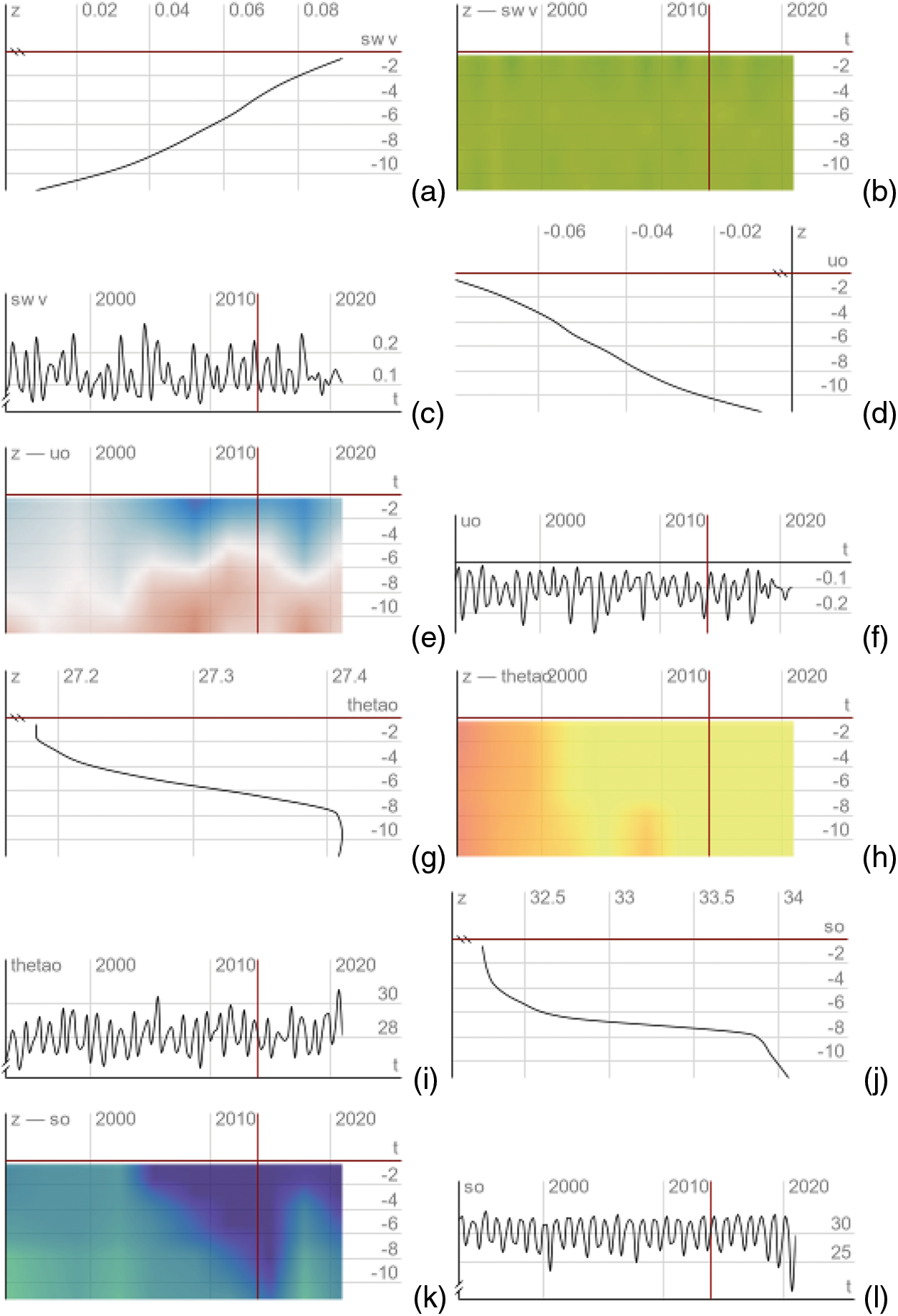
Figure 7: Profiles of (a) depth-seawater velocity (b) velocity-depth over time (c) time-series seawater velocity (d) time-series seawater depth-velocity (e) depth-time for velocity (f) velocity depth-time series (g) temperature-depth (h) temperature depth over time (i) time-temperature (j) salinity-depth (k) salinity-depth over time (l) salinity-depth time series

5.2 Model Results/Behavior

As a first approximation, the present model has been utilized to mimic the horizontal movement and suspension of submerged oil in the water column. The model was initially checked for accuracy by performing a straightforward procedure that consisted of arbitrarily setting the bottom and upper bounds of the computational grid to temperatures of one degree and zero degrees, respectively. As a consequence of this, the temperature gradient that exists between the two boundaries generates a change in density inside the flow, and the variation in density that is brought about by buoyant forces is what brings about the motion within the fluid. Fig. 8 depicts the result of this flow behavior, which shows some convective plumes as expected from a temperature gradient between two plates. This flow behavior is referred to as the Raleigh-Bernard Convection and is one of the most commonly studied flow phenomena in varying fluid flow problems [44–46].

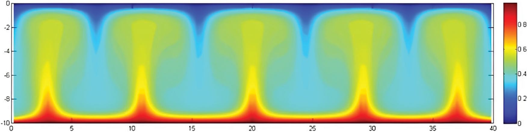
Figure 8: Induced flow behavior between boundaries based on temperature gradient

The model was then used to depict the simulation of a fluid with a lower density penetrating a fluid with a little higher density. Because the fluid concentration was permitted to enter a homogenous computational domain, this is a rudimentary attempt to model the horizontal flow of the oil and its suspension in the water column. Fig. 9a illustrates the computational domain in which the first fluid injection and submergence of the less dense fluid (represented by red color) into the water surface of the somewhat denser fluid (represented by blue color) takes place ten minutes after the discharge of the fluid. The identical fluid injection is shown in Fig. 9b, but 20 min after the initial discharge, it has formed an underwater plume, which is seen floating within the denser fluid while traveling horizontally in the water column. The horizontal movement and extension of the plume are seen in Figs. 9c through 9f. The plume seems to become neutrally buoyant or suspended between the upper mixed layer and the heavier blue color bottom layer as it displaces more of the denser fluid as it moves horizontally, thereby forming a stable layer at a vertical depth of approximately 2–6 meters (this stable layer is the solid, broad, deep red colored band of the oil plume in the Figs. 9a through 9f).

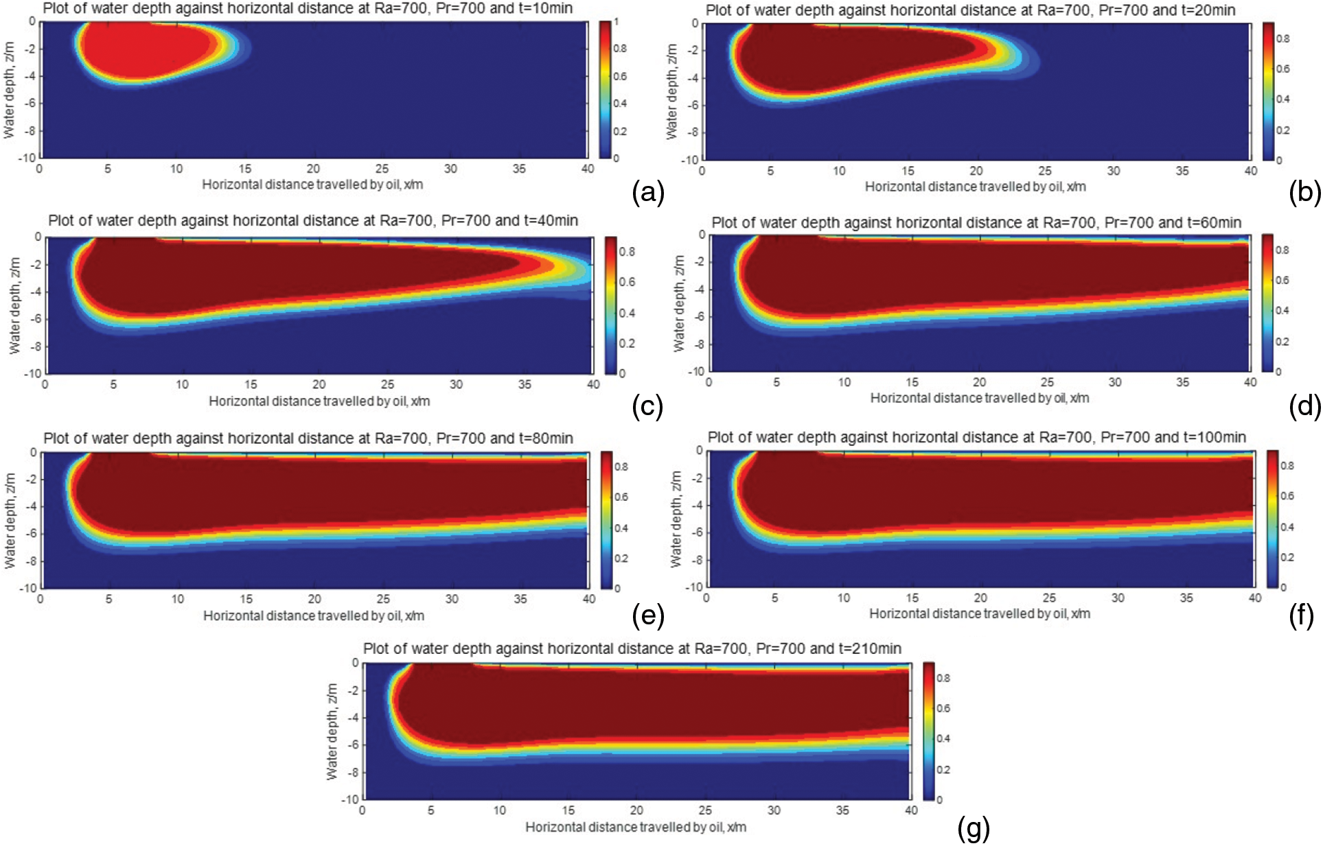
Figure 9: Simulations results plots of Depth (m) on the z-axis against Horizontal distance (m) on the x-axis (a) 10 (b) 20 (c) 40 (d) 60 (e) 80 (f) 100 (g) 210 min

The Fig. 9 Simulations results are the plots of Depth (m) on the z-axis against Horizontal distance (m) on the x-axis showing the behavior of a less dense fluid discharging into a slightly denser ambient domain at different time steps of 10, 20, 40, 60, 80, 100 and 210 min respectively at Raleigh number, Ra = 700 and Prandtl number, Pr = 700. This model was able to capture the neutral buoyant behavior of the heavy bunker C fuel N0.6 oil with a specific gravity of 0.98, which as mentioned earlier, is stated in research as a likely behavior of such heavy oils.

According to the findings of the model, the submerged fluid moved in a horizontal direction of the ambient flow and eventually became entrapped or suspended in the denser fluid at a shallow depth beneath the water surface. This occurred because the submerged fluid appears to have reached a density-sensitive layer with the surrounding ambient water, which resulted in the formation of a pycnocline or terminal layer as shown in Fig. 10. In the present code, a density field is computed to account for the source of the oil deposited at the water surface. At low temperatures, oil will tend to be more viscous than at higher temperatures as viscosity is inversely proportional to temperature and hence the oil might appear to sink beneath the water surface as is demonstrated in the model results. For simplicity at this point in the research, tides, surface water elevation, and bathymetry were not included. From the model result shown in Fig. 10, it can be seen that the submerged oil plume is observed as a dark red long patch or blob within a depth of 2–5 m, where the submerged oil plume lies between the dense (blue colour) heavy water and the mixed layer (lighter colour). More importantly, the simulation shows that as the slightly denser fluid source is deposited at the surface, the blob would submerge below the water surface forming an underwater plume and travel horizontally and become elongated due to the velocity flow from the west boundary which would represent the cross-currents. The simulation plot therefore shows a fair resemblance of the oil behaviour profile in the intermediate field. This model case is a good example for illustrating a buoyancy-driven flow due to convection.

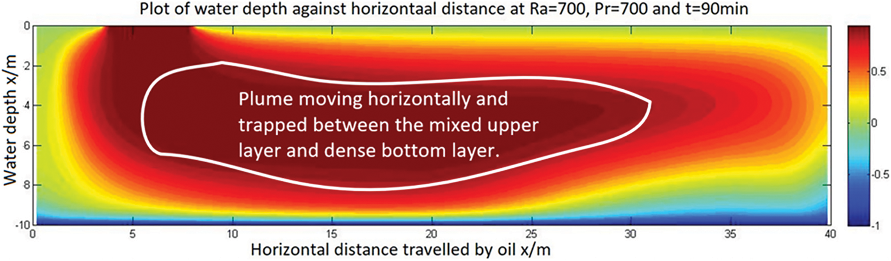
Figure 10: Model simulation showing the suspension of the oil in the water column

The current model result of the specific gravity vs. depth plot is depicted in Fig. 11. According to [47] and [48], the specific gravity should be predicted to decrease with increasing depth, and this graph shows that trend. The map also reveals a stable layer that may represent a pycnocline and is located between one and five meters deep in the sea. This is the potential location where the oil may become trapped. This might potentially confirm, in a very first and rough approximation, the present model’s capacity to capture the behavior of the oil in the intermediate field at a similar depth as reported in the spill event. This would be a validation of the existing model’s ability to capture the behavior of the oil in the intermediate field at a similar depth.

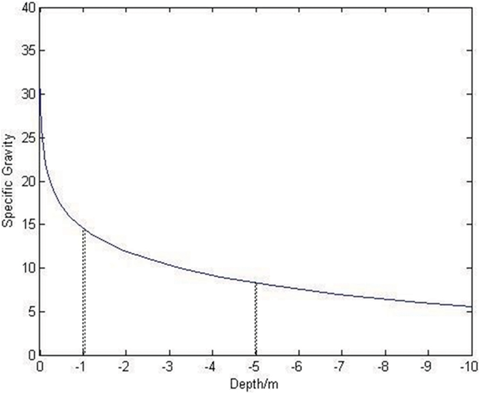
Figure 11: Model plot of the specific gravity vs. depth

Another interesting and qualitative data set from the global analysis and forecast product at 1/12 degree was obtained from the EU Copernicus Marine Environment and Monitoring Service (CMEMS) web portal [28,49] and the related quality information document for Global Ocean Reanalysis Products. Fig. 12 depicts an analyzed vertical temperature profile plot taken very close to the Pointe-a-Pierre oil spill site, revealing a significant stable layer below 5–6 m. This layer appears to occur at a nearly similar depth to the real-life problem and the current model results, and as it demonstrates density variation in the water column, it may have the potential to support the reported observation of the suspended shallow underwater oil plume. In a similar work done by [50] the stable buoyancy of the underwater oil plume layer was determined using a dynamic buoyancy approach.

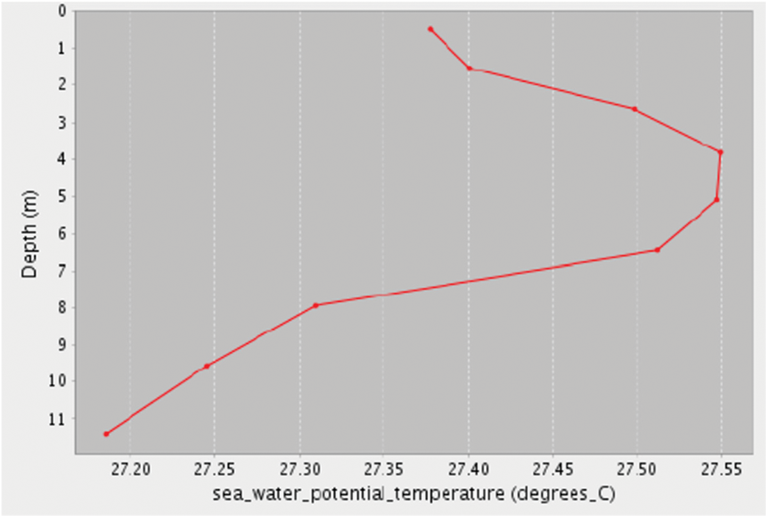
Figure 12: Vertical temperature profile plot in the closest grid point in front of Pointe-a-Pierre. Taken from CMEMS web portal

The novelty of this work, though in its rudimentary stage, is that it has the potential to simulate an oil spill that behaves like a jet at the water surface and then moves through the water column as a plume for a significant horizontal distance. This is a rare form of water surface oil spills, as they are commonly spilled directly on the water surface and move as oil droplets within the water column. Also, most water surface oil spills provide the surface trajectory of the oil spill rather than the underwater trajectory, which is oftentimes simulated by underwater oil spill models [11,51,52].

6  Conclusions

Several interesting oil behaviour phenomena occurred following a surface spill of heavy bunker C fuel into the Gulf of Paria, including oil sinking (near-field), oil becoming neutrally buoyant and moving horizontally (intermediate field), and oil resurfacing (far-field). As a direct consequence of this finding, the focus of this investigation was placed on the intermediate field. In this particular instance, a simplified first-step approach of a two-dimensional CFD numerical model has been created in order to replicate the horizontal motion and suspension of a plume-like oil mass in the water column rather than oil droplets entrained in the water column. This was done in order to accurately describe the situation. The model solves traditional equations for fluid motion by employing the finite difference method. These equations include the continuity equation, the Navier-Stokes momentum and the scalar energy equation. These equations are based on the behavior of fluids. When trying to resolve velocity, pressure, and density fields (as indicated by the utilization of specific gravity), the projection method is the technique of choice.

It has been demonstrated that there is a stable layer in the range of around 2–6 meters below the sea surface, which is reflected in the current model. At this point, it appears that the oil may have been suspended in the water, and the model was able to mimic the overall profile behaviour that was observed throughout the spill event. In addition, a qualitative analysis was performed on the results, and this analysis revealed that the results were in reasonable agreement with the expected connection between specific gravity and depth as, with the data showing the establishment of a pycnocline layer at a water depth of around 1–5 meters. The proposed model is a first attempt and a rough approximation, but it shows the oil to occur at a depth that is comparable to the real-life problem. Additionally, the model has the potential capabilities to simulate and study the behavior of oil movement and neutral buoyancy beneath the water surface, and it suggests that neutral buoyancy can be achieved when the effluent reaches a sensitive density balance layer with the ambient fluid, which puts it in suspension in the water column. More work has to be done to determine the temperature and density pycnocline level at which the oil was confined and pushed horizontally in order to show a more detailed and accurate behavior of the underwater oil plume. This will allow for a more realistic depiction of the behaviour of the oil plume. In addition to this, a greater amount of real data from the spill event and the marine ambient environment of the receiving area has to be employed. The model can be beneficial for informing and aiding in cleanup decisions when the oil flow becomes submerged in the form of an oil plume. The continued presence of oils that are suspended in the water column poses a threat to organisms living in the near-shore coastal waters beneath the watre surface.

Acknowledgement: This study has been conducted using E.U. Copernicus Marine Service Information (http://marine.copernicus.eu/faq/cite-cmems-products-cmems-credit/). The authors acknowledge the Abdus Salam International Centre for Theoretical Physics (ICTP) program for Training and Research in Italian Laboratories in giving author P. Felix the opportunity to spend a visiting period at the National Institute of Oceanography and experimental Geophysics (OGS).

Funding Statement: The authors received no specific funding for this study.

Author Contributions: The authors confirm contribution to the paper as follows: study conception and design: P. Felix, L. Leon, D. Gay; data collection: P. Felix, D. Gay, S. Salon; analysis and interpretation of results: P. Felix, D. Gay, S. Salon, H. Azamathulla; draft manuscript preparation: P. Felix, L. Leon, S. Salon, H. Azamathulla. All authors reviewed the results and approved the final version of the manuscript.

Availability of Data and Materials: Data on which this paper is based is available from the authors upon reasonable request.

Conflicts of Interest: The authors declare that the current study is an extended version of a conference short paper as indicated by reference [50]. This current study emphasizes the underwater buoyancy of the oil plume through thermal driven convection of the oil plume as oppose to the conference paper which described the underwater buoyancy in terms of the dynamic buoyancy.

References

1. Reed, M., Gundlach, E., Kana, T. (1989). A coastal zone oil spill model: Development and sensitivity studies. Oil and Chemical Pollution, 5(6), 411–449. [Google Scholar]

2. Lehr, W., Jones, R., Evans, M., Simecek-Beatty, D., Overstreet, R. (2002). Revisions of the adios oil spill model. Environmental Modelling & Software, 17(2), 189–197. [Google Scholar]

3. ASCE Task Committee on Modeling of Oil Spills. (1996). State-of-the-art review of modeling transport and fate of oil spills. Journal of Hydraulic Engineering, 122(11), 594–609. [Google Scholar]

4. Mishra, A. K., Kumar, G. S. (2015). Weathering of oil spill: Modeling and analysis. Aquatic Procedia, 4, 435–442. [Google Scholar]

5. Reed, M., Johansen, Ø., Brandvik, P. J., Daling, P., Lewis, A. et al. (1999). Oil spill modeling towards the close of the 20th century: Overview of the state of the art. Spill Science & Technology Bulletin, 5(1), 3–16. [Google Scholar]

6. Lehr, W. J. (2001). Review of modeling procedures for oil spill weathering behavior. Advances in Ecological Sciences, 9, 51–90. [Google Scholar]

7. Azevedo, A., Oliveira, A., Fortunato, A. B., Zhang, J., Baptista, A. M. (2014). A cross-scale numerical modeling system for management support of oil spill accidents. Marine Pollution Bulletin, 80(1–2), 132–147. [Google Scholar] [PubMed]

8. Fingas, M., Fieldhouse, B. (2014). Water-in-oil emulsions: Formation and prediction. In: Handbook of oil spill science and technology, pp. 225–270. USA: John Wiley & Sons, Inc. [Google Scholar]

9. Delvigne, G. A. L., Sweeney, C. (1988). Natural dispersion of oil. Oil and Chemical Pollution, 4(4), 281–310. [Google Scholar]

10. Kolluru, V., Spaulding, M., Anderson, E. (1994). A three dimensional subsurface oil dispersion model using a particle based approach. Proceedings of the Arctic and Marine Oil Spill Program Technical Seminar, Canada. [Google Scholar]

11. Yapa, P. D., Wimalaratne, M. R., Dissanayake, A. L., DeGraff, J. A. (2012). How does oil and gas behave when released in deepwater? Journal of Hydro-Environment Research, 6(4), 275–285. [Google Scholar]

12. Korotenko, K. A., Bowman, M. J., Dietrich, D. E. (2010). High-resolution numerical model for predicting the transport and dispersal of oil spilled in the Black Sea. Terrestrial. Atmospheric & Oceanic Sciences, 21(1), 123–136. [Google Scholar]

13. Al-Mebayedh, H. (2014). Oil spill optimized contingency and recovery techniques using ADIOS2. International Journal of Environmental Science and Development, 5(3), 313–316. [Google Scholar]

14. Ansell, D., Dicks, B., Guenette, C., Moller, T., Santner, R. et al. (2001). A review of the problems posed by spills of heavy fuel oils. International Oil Spill Conference, vol. 2001, pp. 591–596. USA, American Petroleum Institute. [Google Scholar]

15. Papadimitrakis, J., Psaltaki, M., Christolis, M., Markatos, N. (2005). Three-dimensional oil spill modelling for coastal waters. Journal of Marine Environmental Engineering, 7(4), 249–379+260. [Google Scholar]

16. Stevens, C. C. (2014). Sinking of hydrocarbon mixtures due to evaporative and/or dissolution weathering on the surface and submerged in water (Ph.D. Thesis). Louisiana State University, USA. [Google Scholar]

17. Wang, S., Shen, Y., Zheng, Y. (2005). Two-dimensional numerical simulation for transport and fate of oil spills in seas. Ocean Engineering, 32(13), 1556–1571. [Google Scholar]

18. Board, M. (1999). Spills of nonfloating oils. USA: National Academies Press. [Google Scholar]

19. Huang, J. C. (1983). A review of the state-of-the-art of oil spill fate/behavior models. International Oil Spill Conference, vol. 1983, pp. 313–322. USA, American Petroleum Institute. [Google Scholar]

20. Wilson, D., Poon, Y. C., Mackay, D. (1986). An exploratory study of the buoyancy behavior of weathered oils in water. Canada: Canada Environmental Protection Directorate. [Google Scholar]

21. de Dominicis, M., Pinardi, N., Zodiatis, G., Lardner, R. (2013). Medslik-II, a lagrangian marine surface oil spill model for short-term forecasting–Part 1: Theory. Geoscientific Model Development, 6(6), 1851–1869. [Google Scholar]

22. Dunnewind, B., Bos, M., Koops, W. (2003). Entrainment of oil from oil spills into the water column: A new theory. International Oil Spill Conference, vol. 2003, pp. 1059–1066. USA, American Petroleum Institute. [Google Scholar]

23. Villoria, C., Anselmi, A., Garcia, F. (1991). An oil spill fate model including sinking effect. SPE Health, Safety and Environment in Oil and Gas Exploration and Production Conference, The Hague, Netherlands, Society of Petroleum Engineers. [Google Scholar]

24. Li, Z. W., Mead, C. T., Zhang, S. S. (2000). Modelling of the behavior of marine oil spills: Applications based on random walk techniques. Journal of Environmental Sciences, 12(1), 1–6. [Google Scholar]

25. Berry, A., Dabrowski, T., Lyons, K. (2012). The oil spill model oiltrans and its application to the celtic sea. Marine Pollution Bulletin, 64(11), 2489–2501. [Google Scholar] [PubMed]

26. Howlett, E., Jayko, K., Spaulding, M. (1993). Interfacing real-time information with OILMAP. Proceedings of the sixteenth Arctic and Marine Oil Spill Program (AMOP) Technical Seminar, Report No. EC/TDTS--94–02286-VOL. 1–2. [Google Scholar]

27. Reed, M., Ekrol, N., Daling, P., Johansen, Ø., Ditlevsen, M. K. et al. (2004). SINTEF oil weathering model user’s manual version 3.0. Norway: SINTEF Materials and Chemistry. [Google Scholar]

28. Chao, X., Shankar, N. J., Cheong, H. F. (2001). Two-and three-dimensional oil spill model for coastal waters. Ocean Engineering, 28(12), 1557–1573. [Google Scholar]

29. Tkalich, P., Huda, K., Hoong Gin, K. Y. (2003). A multiphase oil spill model. Journal of Hydraulic Research, 41(2), 115–125. [Google Scholar]

30. Liu, Z., Chen, Q., Zhang, Y., Zheng, C., Cai, B. et al. (2022). Research on transport and weathering of oil spills in Jiaozhou bight, China. Regional Studies in Marine Science, 51, 102197. [Google Scholar]

31. Canevari, G. P., Calcavecchio, P., Becker, K. W., Lessard, R. R., Fiocco, R. J. (2001). Key parameters affecting the dispersion of viscous oil. International Oil Spill Conference, vol. 2001, no. 1, pp. 479–483. USA, American Petroleum Institute. [Google Scholar]

32. Ooms, G., Segal, A., Van der Wees, A. J., Meerhoff, R., Oliemans, R. V. A. (1983). A theoretical model for core-annular flow of a very viscous oil core and a water annulus through a horizontal pipe. International Journal of Multiphase Flow, 10(1), 41–60. [Google Scholar]

33. Ghosh, S., Mandal, T. K., Das, G., Das, P. K. (2009). Review of oil water core annular flow. Renewable and Sustainable Energy Reviews, 13(8), 1957–1965. [Google Scholar]

34. Xie, B., Jiang, F., Lin, H., Zhang, M., Gui, Z. et al. (2023). Review of core annular flow. Energies, 16(3), 1496. [Google Scholar]

35. United States Environmental Protection Agency–USEPA (2003). Characteristics of spilled oils, fuels, and petroleum products: 1. Composition and properties of selected oils. Report#: EPA/600/R-03/072. [Google Scholar]

36. Ansell, D. V., Dicks, B., Guenette, C. C., Moller, T. H., Santner, R. S. et al. (2001). A review of the problems posed by spills of heavy fuel oils. International Oil Spill Conference, vol. 2001, no. 1, pp. 591–596. Tampa, Florida, USA: American Petroleum Institute. [Google Scholar]

37. Richmond, S. A., Lindstrom, J. E., Braddock, J. F. (2001). Effects of chitin on microbial emulsification, mineralization potential, and toxicity of bunker C fuel oil. Marine Pollution Bulletin, 42(9), 773–779. [Google Scholar] [PubMed]

38. Fritt-Rasmussen, J., Wegeberg, S., Gustavson, K., Sørheim, K. R., Daling, P. S. et al. (2018). Heavy fuel Oil (HFOA review of fate and behaviour of HFO spills in cold seawater, including biodegradation, environmental effects and oil spill response. Copenhagen, Denmark: Nordic Council of Ministers. [Google Scholar]

39. Pryazhnikov, M. I., Minakov, A. V., Guzei, D. V., Pryazhnikov, A. I., Yakimov, A. S. (2022). Flow regimes characteristics of water-crude oil in a rectangular‎ Y-microchannel. Journal of Applied and Computational Mechanics, 8(2), 655–670. [Google Scholar]

40. Chorin, A. J. (1968). Numerical solution of the navier-stokes equations. Mathematics of Computation, 22(104), 745–762. [Google Scholar]

41. Bell, J. B., Marcus, D. L. (1992). A Second-order projection method for variable-density flows. Journal of Computational Physics, 101(2), 334–348. [Google Scholar]

42. Petroleum (2022). API gravity. http://www.petroleum.co.uk/api [Google Scholar]

43. NOAA–National Oceanic and Atmospheric Administration (2009). FACT SHEET: No. 6 Fuel Oil (Bunker C) Spills. U.S. Department of Commerce. NOAA/Hazardous Materials Response and Assessment Division, Seattle, Washington, USA. https://dec.alaska.gov/spar/ppr/response/sum_fy05/041207201/fact/noaa_971_no_6.pdf [Google Scholar]

44. Yu, J. J., Hu, Y. P., Wu, C. M., Li, Y. R., Palymskiy, I. B. (2020). Direct numerical simulations of Rayleigh-Bénard convection of a gas-liquid medium near its density maximum. Applied Thermal Engineering, 175, 115387. [Google Scholar]

45. van der Poel, E. P., Stevens, R. J., Lohse, D. (2013). Comparison between two-and three-dimensional Rayleigh–Bénard convection. Journal of Fluid Mechanics, 736, 177–194. [Google Scholar]

46. Abu-Nada, E. (2011). Rayleigh-Bénard convection in nanofluids: Effect of temperature dependent properties. International Journal of Thermal Sciences, 50(9), 1720–1730. [Google Scholar]

47. Chopra, S., Lines, L. R., Schmitt, D. R., Batzle, M. L. (2010). Heavy oils: Reservoir characterization and production monitoring. Tulsa, Oklahoma, USA: Society of Exploration Geophysicists. [Google Scholar]

48. Price, L. C. (1980). Crude oil degradation as an explanation of the depth rule. Chemical Geology, 28, 1–30. [Google Scholar]

49. COPERNICUS (2022). Quality Information Document for Global Ocean Reanalysis Products GLOBAL_REANALYSIS_PHY_001_030. COPERNICUS, Marine Enviornemntt Monitoring Services. https://catalogue.marine.copernicus.eu/documents/QUID/CMEMS-GLO-QUID-001-030.pdf [Google Scholar]

50. Felix, P. (2020). The underwater trajectory behaviour of heavy oil jet in cross-flow from a broken surface pipeline. The International Conference on Emerging Trends in Engineering and Technology (IConETech-2020), Trinidad, Tobago, The UWI St Augustine. [Google Scholar]

51. Yapa, P. D., Li, Z. (1997). Simulation of oil spills from underwater accidents I: Model development. Journal of Hydraulic Research, 35(5), 673–688. [Google Scholar]

52. Zheng, L., Yapa, P. D. (1998). Simulation of oil spills from underwater accidents II: Model verification. Journal of Hydraulic Research, 36(1), 117–134. [Google Scholar]