A Transient-Pressure-Based Numerical Approach for Interlayer Identification in Sand Reservoirs

1  Introduction

Almost all sandstone reservoirs contain interlayers (i.e., nonpermeable layers in a sandstone layer, as shown in Fig. 1). The presence of interlayers affects the distribution and recovery of petroleum reserves. This phenomenon not only changes the laws of oil and gas occurrence but also alters the laws governing the movement of oil, gas, and water. During oilfield development, interlayers increase the risk of implementing new drilling, increase the difficulty of effectively utilizing remaining reserves, and considerably increase the uncertainty associated with reservoir development [1,2]. The identification and characterization of interlayers are of paramount importance in comprehending the laws governing the migration of oil and gas as well as the distribution of reserves within petroleum reservoirs [3]. Through this understanding, optimizing development plans for oil and gas resources is possible, leading to improved recovery. A comprehensive approach involving the thorough prediction of the spatial distribution of interlayers and their quantitative characterization is required to achieve these objectives.

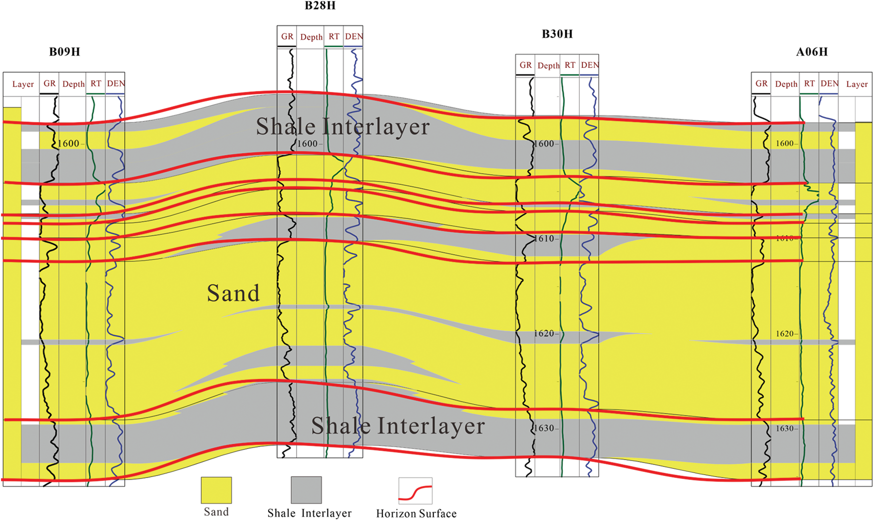
Figure 1: Isolated interlayers in a sand reservoir

In terms of interlayer formations, these formations can be broadly classified into the following three main types: mudstone, calcareous, and other lithologic interlayers. Regardless of the specific type, interlayers provide physical barriers in sandstone reservoirs. Extensive research has been conducted on the identification of interlayers within these reservoirs, with various identification methods available [4,5]. Several methods for identifying and characterizing interlayers are generally available. First, researchers established corresponding sedimentary models based on core observation and description and qualitatively identified interlayers with different mineral contents based on core observation and description through fine interpretation of logging data, empirical statistics, cross-plotting, and other methods [6,7]. Cheng et al. analyzed the origin and vertical distribution characteristics of interlayers using outcrop, core, and logging data and established the correspondence between interlayers and logging curves [8]. Sun et al. used the same method to identify interlayers in a single well, and they derived quantitative formulas for various interlayer sizes based on existing data and quantitatively characterized sand-braided river interlayers [9]. The advantage of this type of method lies in its effective determination of interlayers with different calcium or clay contents and their impact on interlayers. Owing to the impact of the vertical resolution and the thin layer effects of logging data, coupled with the highly heterogeneous nature of subsurface geological conditions, accurately characterizing the thickness and distribution range of interlayers throughout the entirety of a reservoir with limited logging data presents a complex challenge [10]. Meeting the requirements of interlayer recognition for remaining reserve development is difficult due to the prediction accuracy of this method.

The second method is based on seismic data to invert interlayers [11]. Synthetic seismic recording layer calibration is the bridge connecting drilling, logging, and seismic and geological information. Accurate layer calibration gives rich geological significance to abstract seismic profiles [12]. Seismic data are the most commonly used data source in interlayer identification because seismic waves propagate differently in mudstones and sandstones and can be used to identify the position of mudstone interlayers. Dong et al. established a correlation between the gamma logging curve and seismic inversion information, conducted multiparameter lithology inversion, and predicted the spatial distribution characteristics of mudstone interlayers based on this [13]. Cheng et al. achieved fine identification of various interlayers and determination of the interlayer distribution of reservoirs based on seismic inversion and petrophysical facies, respectively [14]. Zhou et al. combined seismic data, drilling data, and sedimentary evolution rules to identify and predict different types of mudstones using high-frequency expansion processing and acoustic impedance inversion technologies to predict thin mudstone interlayers [15]. The position of the development of mudstone interlayers mainly shows differences in lithology, density, and sound velocity compared with the surrounding rocks. The pronounced amplitude of mudstone on the seismic profile indicates mudstone interlayers, which can be accurately identified based on the physical properties of mudstone. The superior lateral resolution of seismic data helps overcome the issue of inadequate well control, while its high longitudinal predictive accuracy enables the identification of interlayers with a thickness of as little as 0.5 m [16,17]. The main disadvantage of this method lies in the high cost of conducting large-scale 3D seismic work, and many oil fields that enter the later stages of development are difficult to afford. Moreover, seismic interpretation is a complicated task.

The third method is to use machine learning methods. With the popularization of artificial intelligence technology, numerous geologists are attempting to utilize machine learning methods and neural network technology to solve geological problems [18–20]. Al-Mudhafar applied probabilistic neural networks to the lithofacies sequences of the well-logging construct [21]. They then established the nonlinear relationship between core permeability, well-logging data, and lithology using a generalized boosting regression model, which was utilized to study the distribution of interlayers. However, the foundation of machine learning lies in sufficient sample points. Most interlayer samples in oilfields are limited, and the large discrepancy in the number of samples between different categories of interlayers decreases the effectiveness of conventional machine learning algorithms in classification [22]. Simultaneously, logging-based and machine learning methods can only determine whether the reservoir encountered by the well contains interlayers. These methods are incapable of detecting interlayers outside the well.

Inspired by the concept of utilizing pressure response for interpreting reservoir parameters in well-testing theory [23,24] and considering the limitations of the aforementioned interlayer identification methods, a novel approach to identifying interlayers using transient bottom-hole pressure data during well testing is introduced. Regardless of the stage of oilfield development, this method depends solely on transient pressure data collected during well testing and can accurately determine the distribution of interlayers around the wellbore with minimal expense. This study is of considerable importance for improving the quantitative identification of interlayers and reducing uncertainty in the oilfield development process.

2  Methodology

2.1 Theoretical Background

Given the reservoir, fluid, and gas well parameters, the bottom-hole pressure and production of a gas well can be obtained through reservoir simulation or other reservoir engineering methods. However, the physical characteristics of underground reservoirs are often unknown in practice. The accurate data that can be obtained only includes the production and pressure of oil wells and other small amounts of known information. Well-testing theory provides a method to invert effective reservoir parameters (such as permeability, skin factor, wellbore storage coefficient, or distance between well and fault) within the production well flow region using the production and pressure data of oil wells, which has been widely used in the petroleum industry [25,26]. Fig. 2 shows the basic workflow of well testing. After obtaining the production and pressure data of the oil well, the log-log curve is calculated and fitted with the standard chart of the interpretation model to calculate the reservoir parameters inversely. Various methods, including analytical and numerical methods, are used to obtain the interpretation model of well testing.

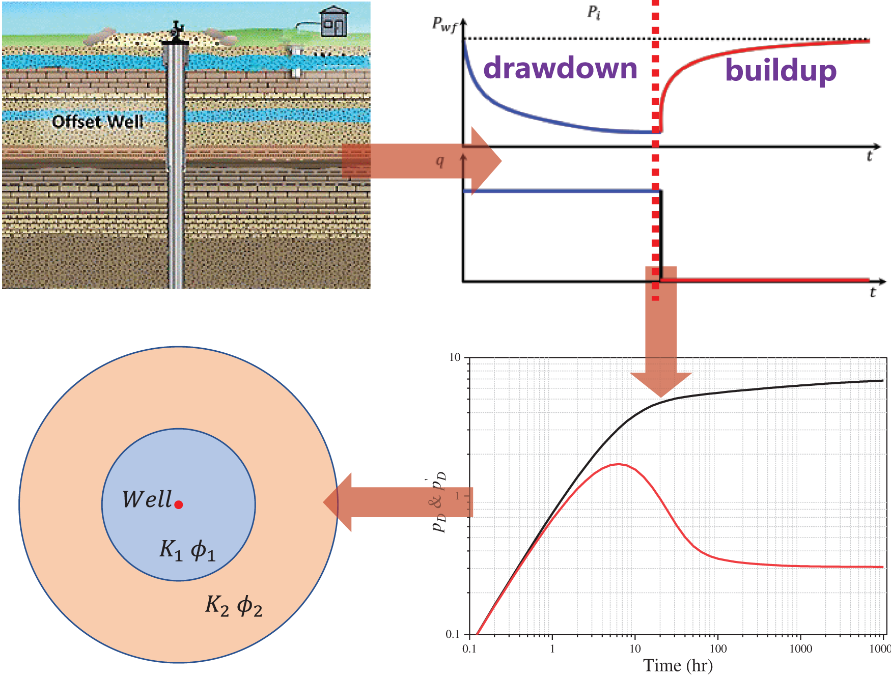
Figure 2: Workflow of a typical well test

Inspired by the theory of well testing, the production and pressure responses of an oil well is one-to-one correspondence. In sand reservoirs with interlayers, the production and pressure of a well encountering interlayers will change correspondingly when the thickness or distribution of the interlayer changes. As long as we can find the pressure response law when the interlayers change, we can deduce the characteristics of the interlayers when the pressure response features are known.

The identification of interlayers mainly relies on the characteristics of the infinite acting radial flow (IARF) of the fluid. Planar radial flow is the most common type of unstable flow. The oil well is perforated throughout the entire formation, and after production starts, the fluid in the formation flows horizontally from all directions toward the wellbore. On any horizontal plane perpendicular to the wellbore in the formation, the fluid always flows towards the wellbore from all directions, and this flow is called IARF, or radial flow for short, as shown in Fig. 3a.

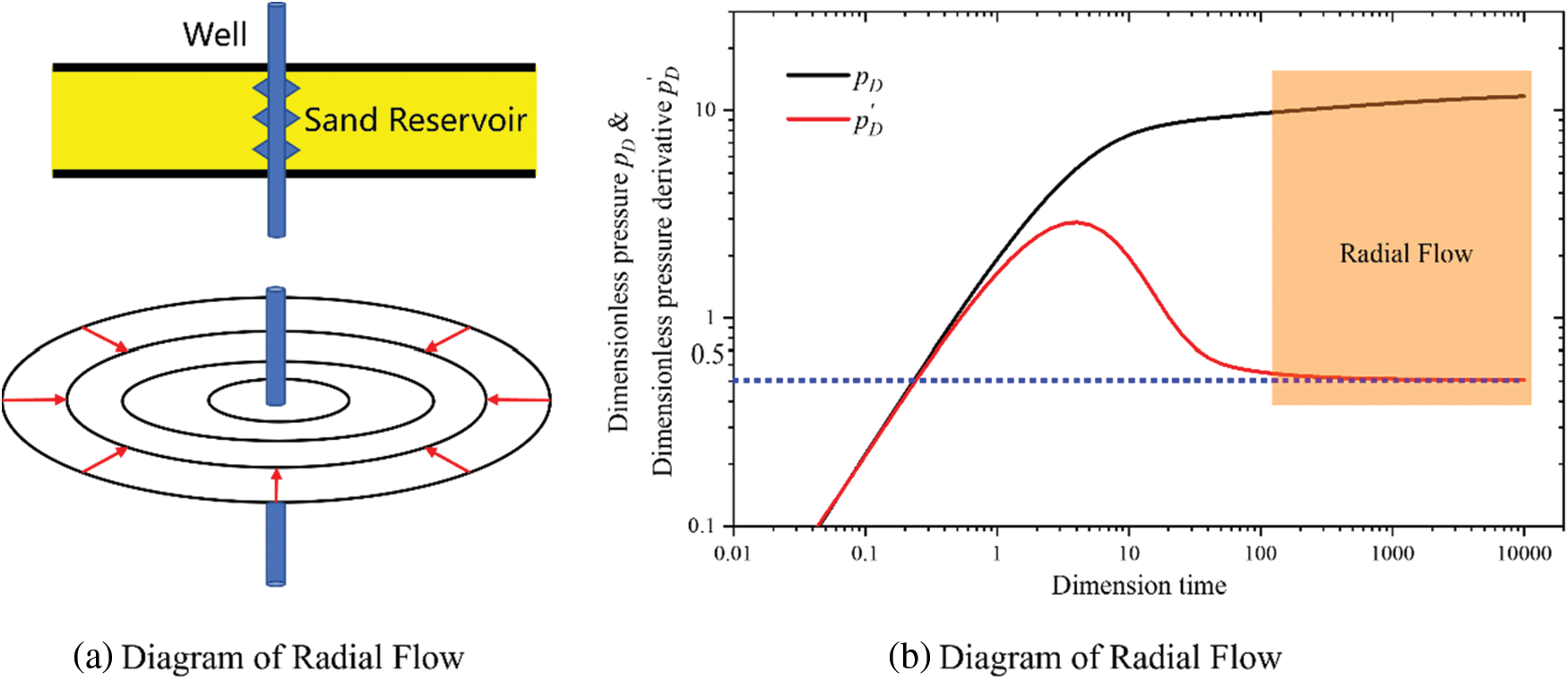
Figure 3: Schematic of radial flow and its characteristics in a log-log curve

The dimensionless pressure of IARF can be expressed by the following formula (for the detailed derivation, please refer to Section 2 of literature [27]),

pD=0.5(ln⁡tD+0.80907+2S) (1)

where pD is dimensionless pressure, tD is dimensionless time, and S (-) is the skin factor.

The dimensionless pressure derivative dpD′ of IARF can be expressed as

dpD′=dpDdln⁡tD=0.5 (2)

Therefore, the main characteristic of radial flow on a log-log curve lies in the representation of the derivative line segment as a horizontal straight line. On dimensionless coordinates, the ordinate value of the horizontal line is exactly 0.5, as shown in Fig. 3b.

When interlayers exist in the reservoir, the fluid flow will no longer follow the flow law of radial flow, and the double logarithmic curve of the pressure response will no longer be a horizontal straight line. Currently, the pressure response chart is established under different interlayer parameters. The actual oil well transient pressure data can be fitted with the standard chart to obtain the parameters of the interlayer.

The analytical, semi-analytical, and numerical methods are used to obtain the well-testing interpretation model and its typical chart. Remarkably limited analytical solutions can often only be obtained due to the complexity of actual geological models. Numerical well testing is considered the best method for obtaining well-testing models under complex geological conditions. The following will explain how the numerical method is used to obtain the calculation model of the interlayer parameters.

2.2 Physical Model

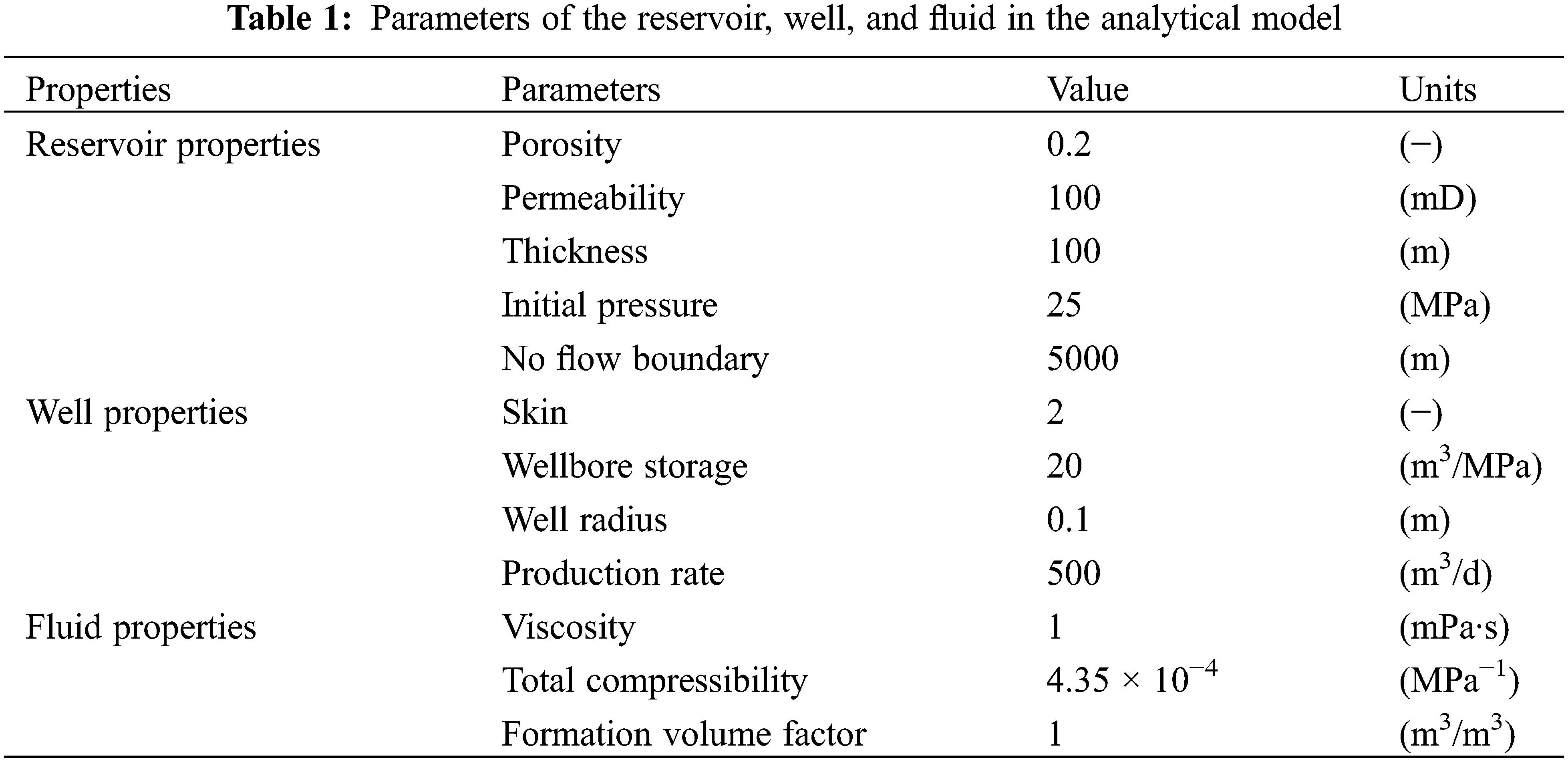
For the sake of simplification, the physical model of the interlayer is expressed as an interlayer with a certain thickness in the sandstone reservoir, as shown in Fig. 4. Oil wells only encounter sandstone reservoirs, and a certain distance is observed from interlayers. The thickness of the sandstone reservoir is known, while the position and thickness of the interlayer are positional. The model initially contains only single-phase fluids. Herein, the direction parallel to the well and the interlayer is defined as the I direction, and that perpendicular to the well and the interlayer is defined as the J direction. Gravity is ignored in the calculation. Specific parameters for fluids, reservoirs, and wells are presented in Table 1.

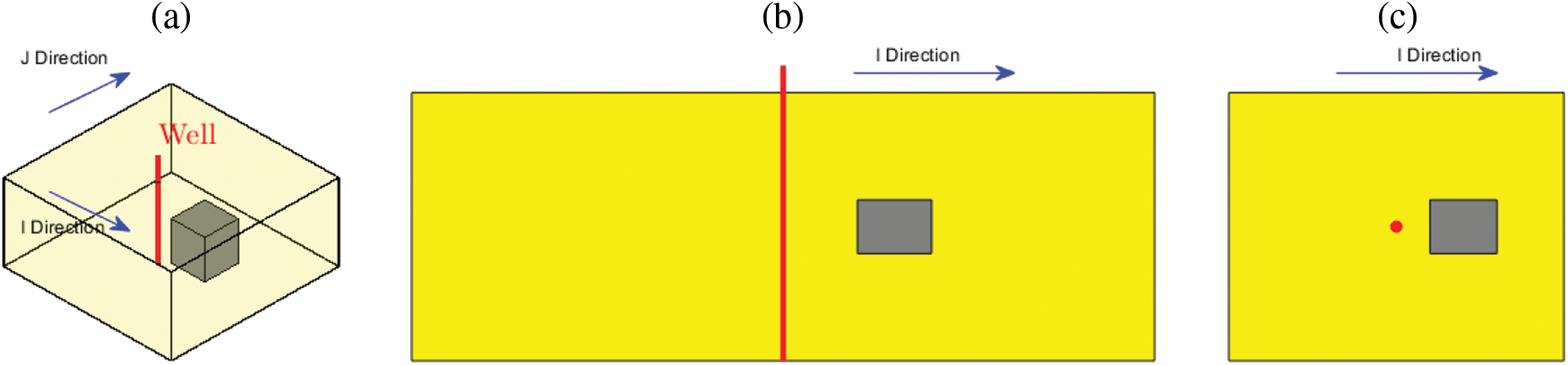
Figure 4: Physical model of the interlayer in a sand reservoir. (a) Reservoir model. (b) A front view of the reservoir profile. (c) A top view of the reservoir profile

2.3 Governing Equation

In a sandstone reservoir with interlayers, the mass conservation equation for single-phase flow is expressed as

∂(ϕρ)∂t+∇⋅(ρv→)=ρq (3)

where ϕ (−) is the reservoir porosity, ρ (kg/m3) is the fluid density, v→ (m/s) is the fluid velocity, and q (m3/s) is the source-sink term.

Eq. (3) contains more unknowns than the formula. Constitutive equations must be introduced to provide the relationship between different states of the system (pressure, volume, and temperature) and derive a closed mathematical model. The velocity of the flow is modeled using Darcy’s law.

v→=−Kμ∇p (4)

where K (m2) is the reservoir permeability, μ (mPa·s) is the hydrodynamic viscosity, and p (MPa) is the fluid pressure.

Assuming that the fluid has constant compressibility, the compressibility of the fluid is constant and independent of pressure, the following is obtained:

ρ=ρ0ecf(p−p0) (5)

where cf (1/MPa) is the compressibility coefficient of the fluid, and ρ0 (kg/m3) is the original density of the fluid. Eq. (5) holds for most liquids that do not contain significant amounts of dissolved gas.

Describing the fluid behavior by only relying on the above equations is difficult. Therefore, the conditions for the behavior of the outer boundary should also be determined. Mathematically, the nonflow condition across the outer boundary is modeled by specifying a homogeneous Neumann condition, which can be expressed as

v→⋅n→=0 (6)

where n→ (−) is directional derivative of the normal outside the boundary.

The initial conditions for the initial state of the fluid system are expressed as follows:

p(z0)=p0 (7)

where p0 (MPa) is the initial reservoir pressure.

Wells typically produce oil at a constant production rate or pressure. The well model mainly aims to accurately calculate the radius pressure of the well when the injection or production rate is known. Well flow is proportional to the pressure drop near the well; thus, the flow rate of the well can be obtained using the following equation:

qw=J(pR−pw) (8)

where qw (m3/s) is the flow rate of the well. J (m3/s/MPa) is called the productivity index for production wells, which takes into account all rock and fluid properties and geometric factors affecting flow. pR (MPa) is the reservoir pressure, and pw (MPa) is the pressure at the well connection.

The well flow rate when considering the wellbore storage effect is expressed as

qw=J(pR−pw)+C∂pw∂t (9)

where C (m3/MPa) is the wellbore storage coefficient.

The Peaceman model was used to describe the productivity index of vertical wells,

WI=Khln⁡(rerw)+S (10)

where h (m) is the perforation thickness of the well, re (m) is the effective radius, rw (m) is the diameter of the well, and S (−) is the skin factor of the well.

Given a geological model of the interlayer, the production and pressure of an oil well can be determined by discretely solving the equations through the finite volume method. The physical model and simulation were performed on the MATLAB Reservoir Simulation Toolbox (MRST). MRST is a free, open-source software for reservoir modeling and simulation based on the finite volume method. However, MRST offers quite comprehensive black oil and compositional reservoir simulators capable of simulating industry-standard models and also contains graphical user interfaces for postprocessing simulation results [28].

2.4 Obtaining the Log-Log Curve

In well test theory, the abscissa of the log-log curve is usually time, and the ordinate is usually pressure difference and differential pressure derivative. Therefore, there are often two curves in the double-logarithmic curve, one is the pressure difference vs. time curve, and the other is the pressure difference derivative vs. time curve. The differential pressure is calculated as follows:

Δp(t)=p0−p(t) (11)

The pressure difference derivative refers to the rate of change in the pressure difference over time. In well test analysis, pressure difference derivative is defined as the derivative between the natural logarithm of differential pressure and time, which is defined as

dp′=dΔpd(ln⁡t)=dΔpdt⋅t (12)

The pressure difference derivative is calculated numerically. There are many methods to calculate the derivative, such as difference quotient, interpolation polynomial, and cubic spline function derivative methods. The method proposed by Bourdet is widely used in well testing. The calculation formula of pressure derivative at the i-th pressure difference is

(dpdln⁡t)i=[(Δpi−1Δln⁡ti−1)Δln⁡ti+1+(Δpi+1Δln⁡ti+1)Δln⁡ti−1]Δln⁡ti−1+Δln⁡ti+1 (13)

Dimensionless pressure and time are often used to simplify calculations and obtain a map for all formations in the well test. Eq. (1) represents the relationship between dimensionless pressure (actually dimensionless pressure difference, under the conventional name, here still called dimensionless pressure) and dimensionless time. We did the same thing. Dimensionless time and dimensionless pressure are defined as [29]

tD=KϕμCtrw2⋅t (14)

pD=KhΔpqμB (15)

where Ct (1/MP) is the comprehensive compression coefficient, q (m3/s) is the stable production of the well before shut-in, and B (m3/m3) is the oil volume coefficient.

2.5 Calculation of the Interlayer Parameters

The true log-log and theoretical log-log curves are fitted to obtain the interlayer parameters. First, the theoretical curves of the interlayer with different parameters are obtained using the numerical model. Subsequently, the logarithmic curve of the actual well is fitted against the theoretical curve, yielding specific parameters of the interlayer. A schematic of the calculation process is presented in Fig. 5. The fitting workflow involves the curve fitting in well-testing theory, and the details can be found in references [27].

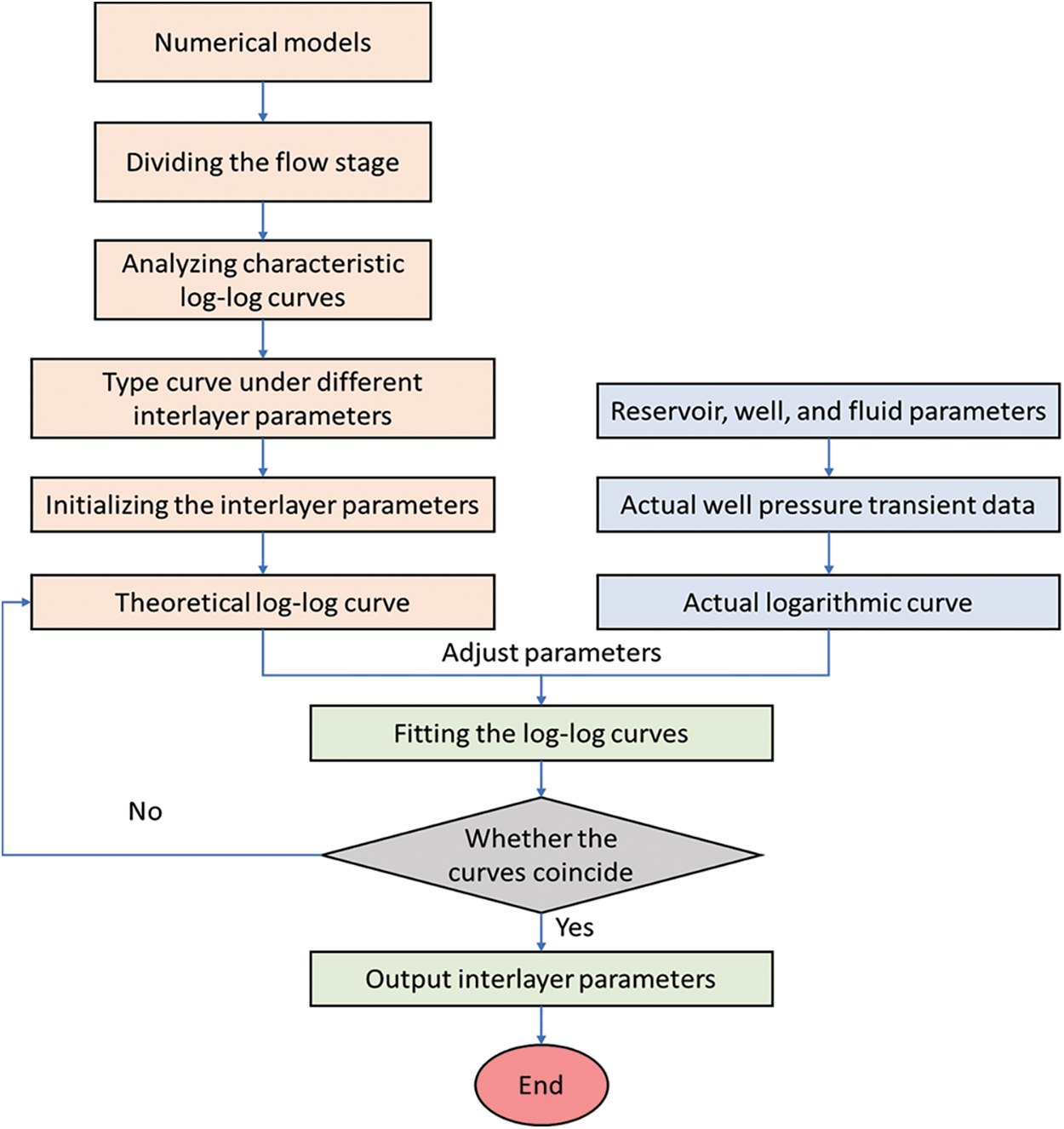
Figure 5: Workflow of calculating interlayer parameter

3  Model Verification

The proposed model is verified by comparing it with the analytical solution for radial flow. Obtaining analytical solutions to mathematical models with interlayers is difficult. The analytical and numerical solutions without the interlayer are compared to validate the numerical model. The analytical model without the interlayer is represented as a finite rectangular reservoir with a reservoir radius re . A vertical well sits in the center of the reservoir and is perforated throughout the reservoir. The formation contains a slightly compressible, single-phase fluid with constant fluid viscosity and compressibility. Parameters related to the reservoir, well, and fluid for simulation and analytical solution are shown in Table 1.

The analytical solution of the radial flow with a closed boundary has been previously proposed in the petroleum industry. Many pieces of literature have derived the pressure response for radial flow [27]. The analytical solution of the model in pull space is expressed as

p¯D=1u(f(u)[I1(f(u))K1(reD(f(u)))+K1(f(u))K0(reD(f(u)))]I0(reDf(u))K0(f(u))−I0(f(u))K0(reDf(u))+S) (16)

and,

f(u)=uCDe2S (17)

where u is the variable of Laplace space, CD is the dimensionless wellbore storage, reD is the dimensionless reservoir radius, I0 and I1 are the zero-order and first-order modified Bessel functions of the first kind, respectively. K0 and K1 are zero-order and first-order modified Bessel functions of the second kind, respectively.

Through the Stehfest numerical inversion algorithm [30], the pressure in the Laplace space in Eq. (16) can be transformed into the relationship between time and pressure in the real space,

pD(tD)=ln⁡2tD∑i=1nVip¯D(ln⁡2tDu) (18)

where Vi is a coefficient related to the number of items N .

Fig. 6 presents the comparison between the proposed model and the analytical solution. The upper and lower lines represent the dimensionless pressure and the dimensionless pressure derivative (same as all log-log curves shown below), respectively. Herein, the numerical model is in good agreement with the analytical solution, which shows its reliability. The ordinate value corresponding to the green horizontal line in the figure is 0.5, which is consistent with the radial flow characteristics mentioned above.

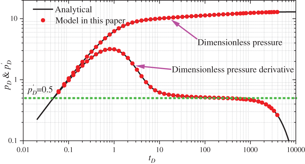
Figure 6: Comparison between the solution of the proposed model and the analytical solution

4  Results and Discussion

4.1 Typical Log-Log Curves

The model is adjusted to the physical model of interlayers in Section 2.2 to illustrate the influence of interlayers on fluid flow in sandstone reservoirs. The oil well in the center of the reservoir is initially produced at a constant rate of 2000 m3/d for 90 days, and then the well will build up for 20 years (to obtain the entire pressure response stage in the buildup and the pressure buildup in the field is only dozens of days). The reservoir parameters are consistent with the analytical model in the verification part, and the specific parameters of interlayers, wells, and fluids are presented in Table 2.

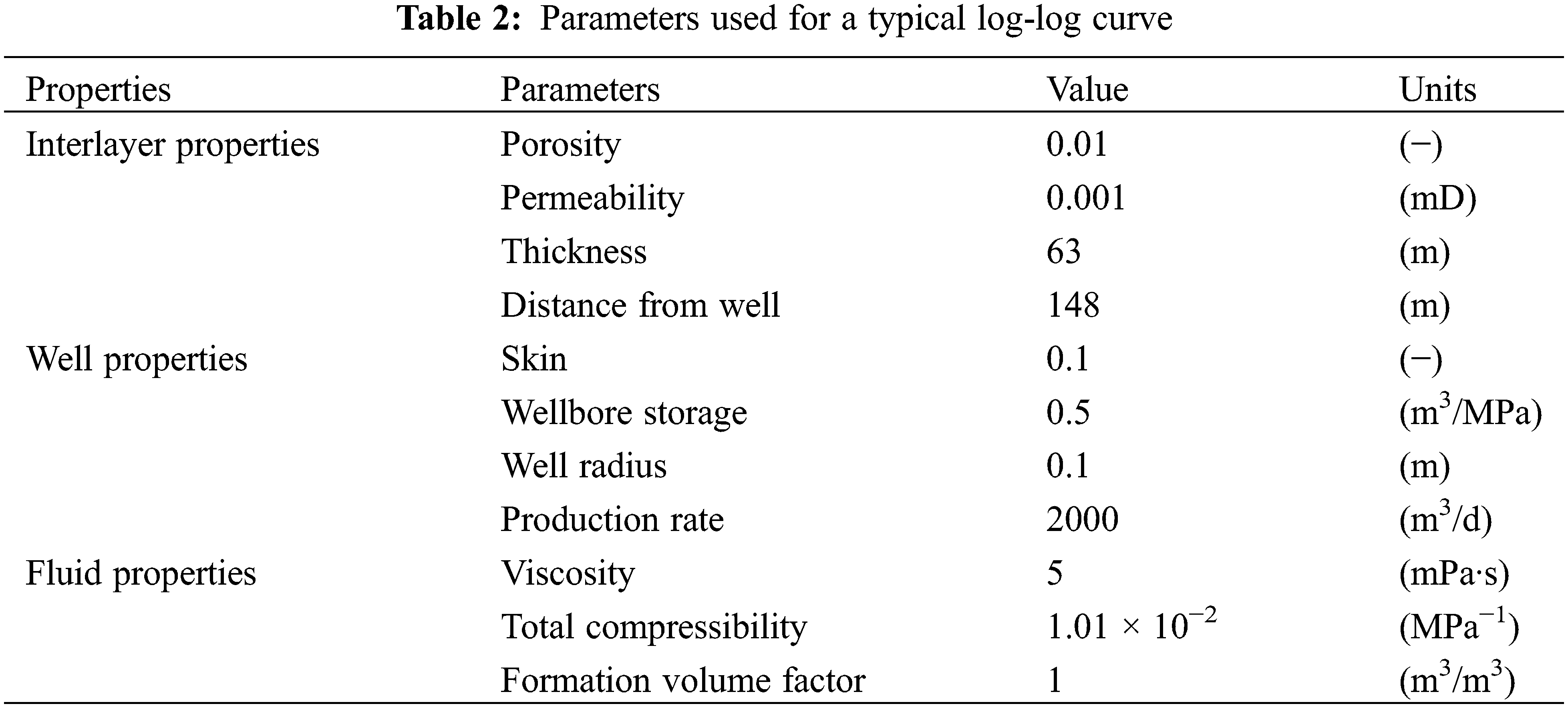
Fig. 7 shows a typical log-log pressure buildup curve in the reservoir with and without an interlayer. Notably, nondimensional graphs are not used in this study to correspond with actual flow time. The log-log curve with interlayers is consistent with the shape of the log-log curve of superimposed sand bodies reported by Zhang et al. [31]. The main feature is that the pressure derivative curve moves upward when the pressure build-up spreads to the interlayer. The pressure response with interlayers can be divided into the following five stages on the log-log curve.

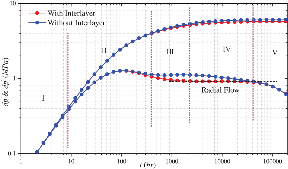
Figure 7: Typical log-log curve and flow stage division when the interlayer exists in sand reservoirs

Stage I: The first stage involves wellbore storage, which is attributed to the compressibility of the fluid. The difference between the surface and bottom-hole rates emerges after the well is closed and the wellbore is filled with fluid.

Stage II: The second stage is the skin and transitional flow stage, where the skin effect reflects the change in permeability near the wellbore. During this stage, the bottom-hole rate gradually approaches the surface rate and then decreases to zero when the well is closed. Simultaneously, the pressure derivative starts to respond to the baffles, and the pressure derivative curve shifts upward.

Stage III: The third stage is the interlayer blocking stage, before which the pressure has not yet completely crossed the interlayer and the interlayer hinders pressure propagation. Compared with the case without the interlayer, the derivative curve shifts upward in the case with the interlayer. Thus, the interlayer has the largest impact during this stage.

Stage IV: In the fourth stage, the pressure propagates across the interlayer. Compared with the previous stage, the amplitude of the pressure recovery decreases and the pressure derivative curve shifts downward in this stage.

Stage V: The fifth stage is the boundary response stage, where the pressure propagates to the boundary and the pressure derivative falls back.

Overall, in the wellbore and skin stages, the pressure response with an interlayer behaves similarly to that without the interlayer before the interlayer is detected. When the pressure has already reached the interlayer in the late stage of production (Fig. 8), the interlayer is immediately detected after the end of the wellbore and skin stages during pressure recovery, and the pressure derivative immediately shifts upward (i.e., at the end of Stage II). At this stage, the pressure boundary has not yet exceeded the right boundary of the interlayer. Therefore, the boundary between Stages II and III is the right boundary of the interlayer. The pressure has already reached the right side of the interlayer when the pressure boundary exceeds the boundary of the interlayer, but the pressure derivative continues to shift upward (Stage III). The pressure quickly propagates through the reservoir on the right side of the interlayer after completely crossing the interlayer, and the pressure derivative shifts downward (Stage IV). The pressure derivative behaves similarly to that without an interlayer after the pressure has reached the boundary (Stage V). The pressure response cloud maps for each stage during pressure recovery are shown in Fig. 8.

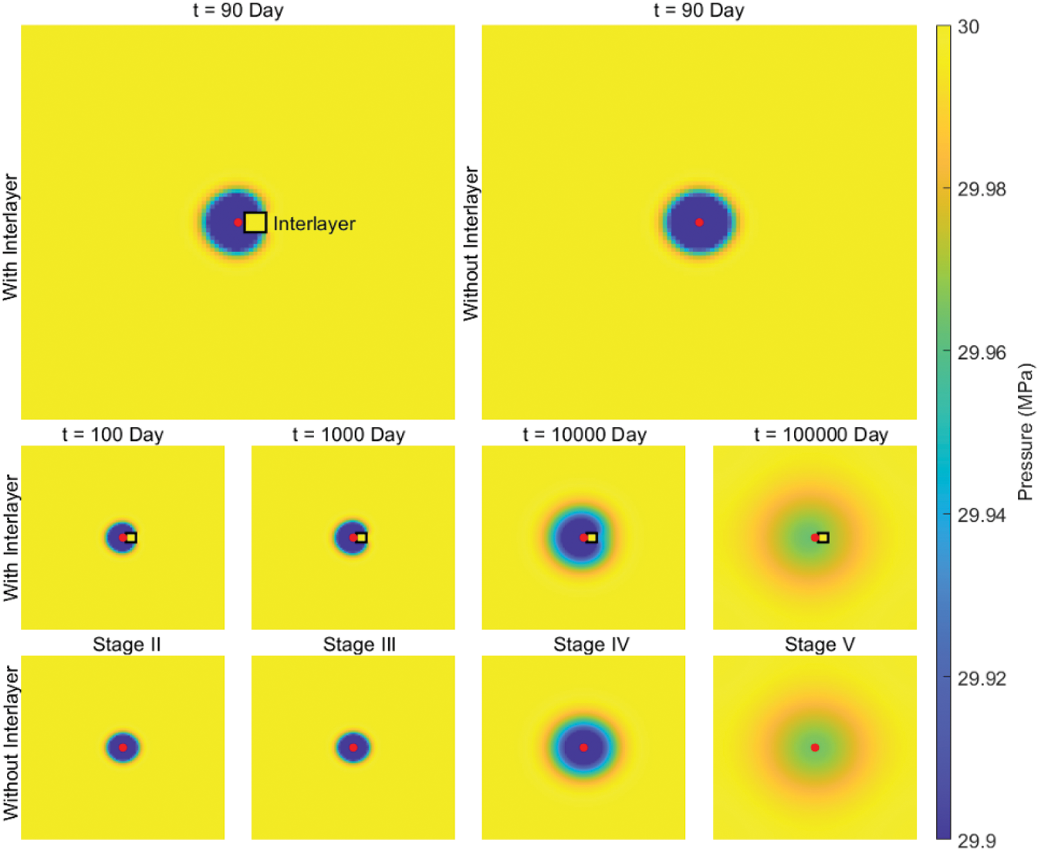
Figure 8: Pressure distribution at different stages. The top is with the interlayer, the bottom is without the interlayer. The black rectangle represents the interlayer, and the red dot represents the oil well

4.2 Impact of Interlayer Thickness

In practice, the thickness of the interlayer in the reservoir ranges from a few meters to tens of meters. The thickness of the entire model is 100 m. The log-log curves are simulated when the interlayer thickness is 27, 63, and 72 m. Fig. 9 shows the influence of different interlayer thicknesses on the log-log curve. The peak pressure derivative changes from 1.02 to 1.17 when the thickness increases from 27 to 63 m. As the interlayer thickness increases, the pressure derivative does not change in the first and second stages, gradually shifts upward in the third and fourth stages, and completely coincides in the fifth stage. The thickness of interlayers primarily influences the third and fourth stages of fluid flow. Furthermore, a thick interlayer results in rapid pressure recovery and upward curve movement. The thickness of the interlayer only impacts the peak value of the pressure derivative in the fourth stage, with thick interlayers corresponding to high peak values.

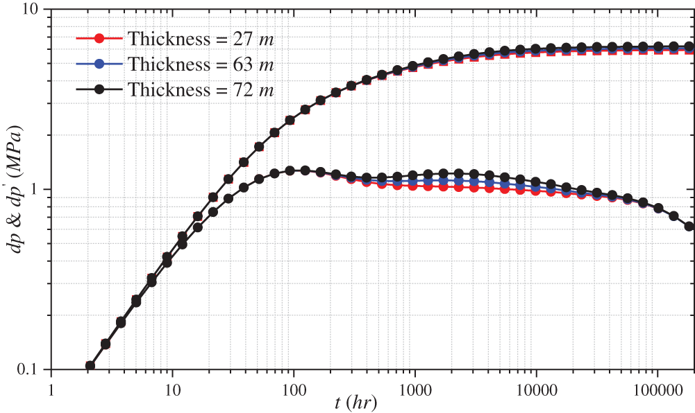
Figure 9: Effect of different interlayer thickness on the log-log curve

4.3 Impact of Interlayer Distance

Fig. 10 shows the sensitivity of the distance between the oil well and the interlayer. The effect of distance on pressure behavior is similar to that of a single closed fault before the pressure crosses the interlayer. The thickness of the interlayer is set similarly to that of the reservoir to effectively understand the effect of the distance between the interlayer and the oil well on pressure response. The presence time of the interlayer in the log-log curve extended from 297 to 533 h when the interlayer distance increased from 148 to 267 m. The control group is t/r2 for any radial diffusion problems. Doubling the distance increases the boundary detection time by four. This relationship applies to all boundary problems and the interlayer problem in this study. Therefore, the appearance of the third stage is delayed as the distance between the interlayer and the oil well increases. The delayed time is proportional to the square of the distance. Overall, the pressure recovery is slow when the interlayer is far away and the curve moves downward. The distance between the interlayer and the oil well only affects the appearance time of the third stage and not its duration.

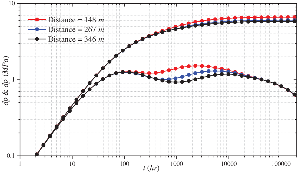
Figure 10: Effect of different interlayer distance on the log-log curve

4.4 Impact of Interlayer Width

Figs. 11 and 12 show the effects of different interlayer widths in various directions on the log-log curve. The log-log curve does not change as the interlayer width increases in the I direction. This phenomenon is due to the formation of a pressure isolation zone during the pressure propagation process by the preceding interlayer, hindering pressure propagation. The subsequent interlayer does not play any role.

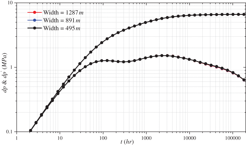
Figure 11: Effect of different interlayer width on the log-log curve along the I direction

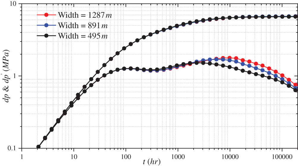
Figure 12: Effect of different interlayer width on the log-log curve along the J direction

However, as the interlayer width in the J direction increases, the hindrance to pressure propagation increases, and the pressure derivative curve moves upward. The increase in width does not affect the first and second stages but significantly impacts the duration of the third stage. A wide interlayer prolongs the pressure derivative upturn. The time when the pressure reciprocal is no longer upturned is proportional to the width of the interlayer. When the interlayer width increases from 495 to 1287 m, the disappearance time of the pressure derivative upturn increases linearly from 2289 to 13157 h.

5  Field Application

M Oilfield has multiple sets of sandstone reservoirs developed vertically. The research area has drilled different numbers of wells at various times to develop different layers. As of December 2022, the drilling locations in the research area are shown in Fig. 13. A16 is a vertical well drilled in the N formation and was put into production in December 2018. This well underwent a pressure buildup test in January 2019. The known reservoir, fluid, and well parameters are shown in Table 3. The log-log curves of the pressure buildup test are shown in Fig. 14. Core results and log interpretation (Fig. 15) indicate that no interlayer was encountered in the reservoir during drilling. However, the pressure derivative log-log curve of the pressure buildup test shows a slight increase, indicating the presence of the interlayer near the wellbore.

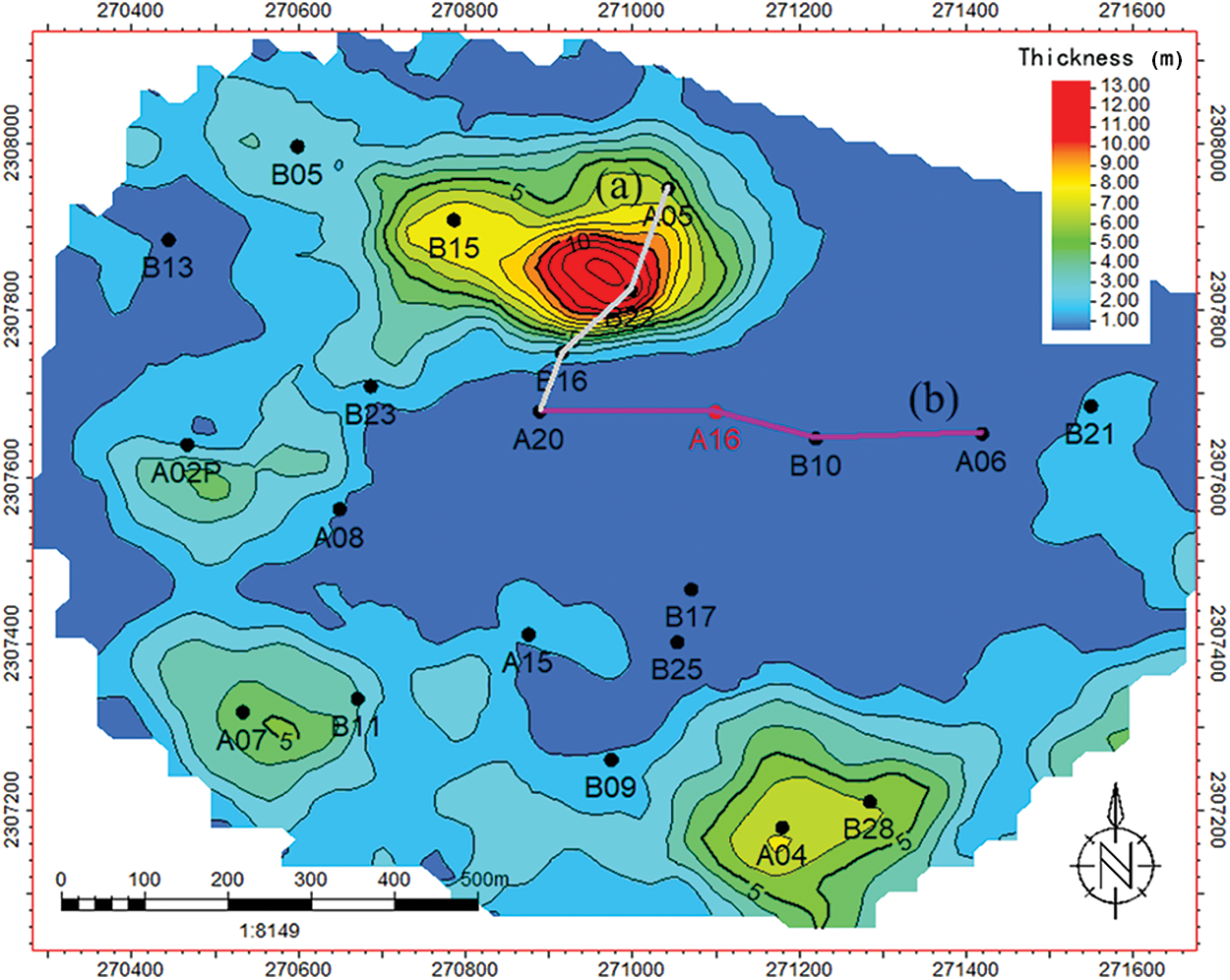
Figure 13: Interlayer thickness plan of the study area

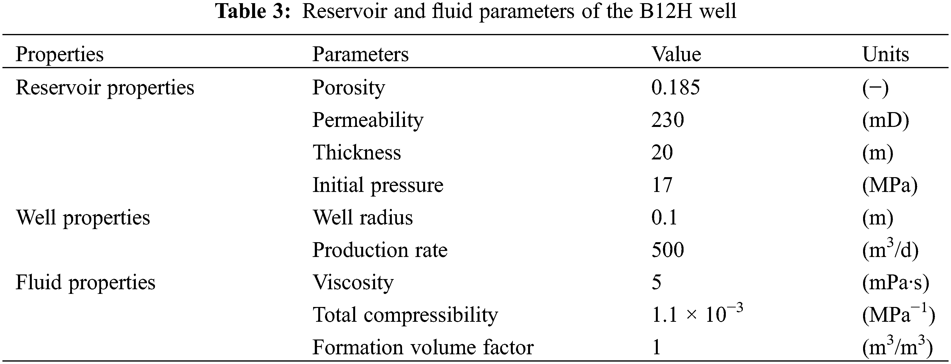
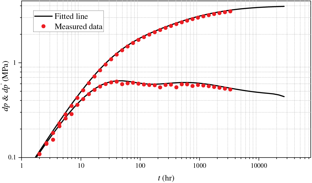
Figure 14: Log-log curve for bottom hole pressure of well A16

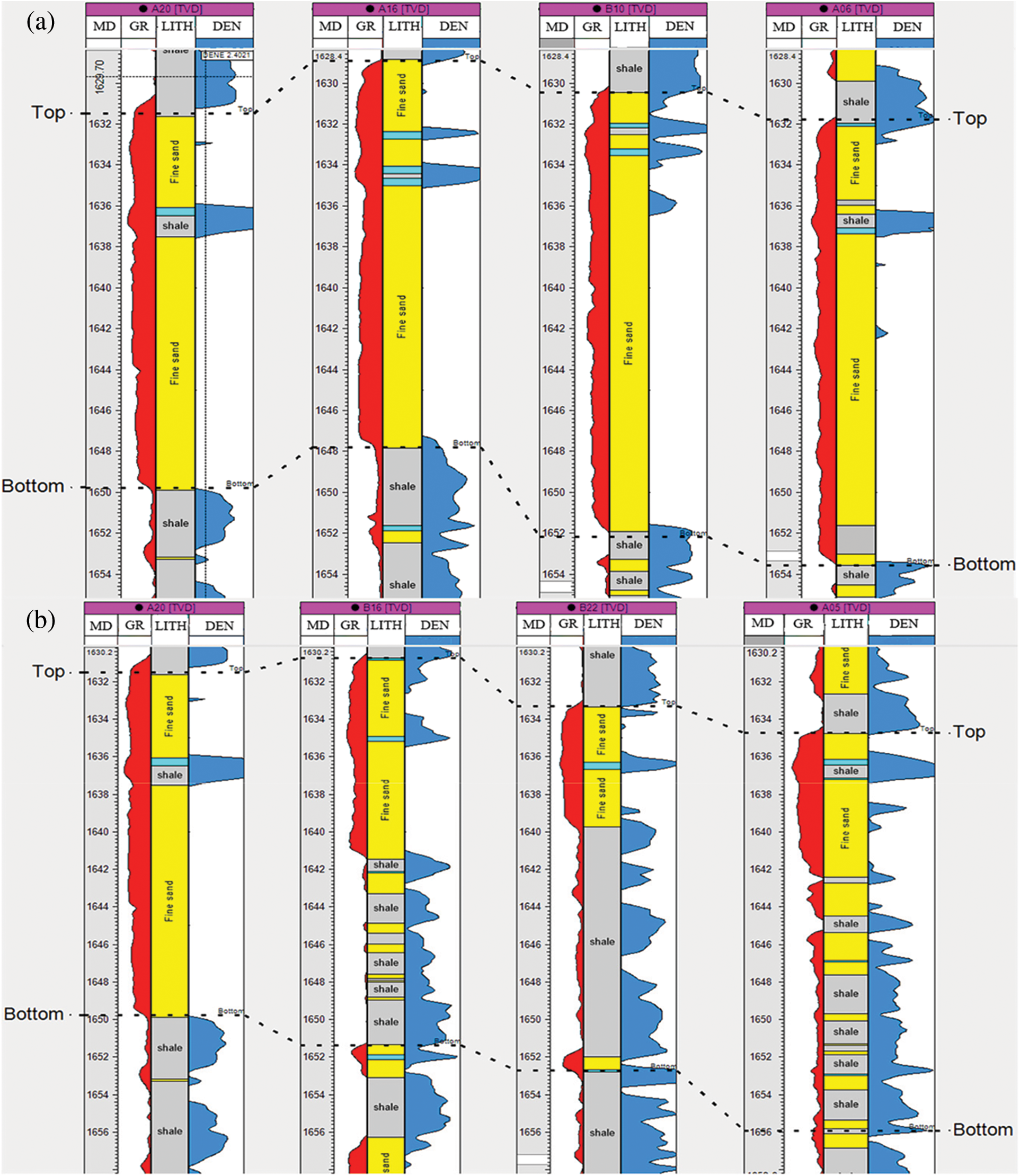
Figure 15: Well sections of two lines in the study area. The dotted lines in the figure indicate the top and bottom of sandstone reservoirs

Using the calculation method for the aforementioned interlayer parameters and fitting to the typical log-log curves, an existing interlayer layer with a thickness of approximately 12 m was calculated around 150 m from well A16. Fig. 15 shows a continuous well-to-well cross-section of two lines in the study area. The well-to-well cross-section from A20 to A06 shows that the sand below the cross-section is continuous and no interlayer exists. However, the well-to-well cross-section from A20 to B22 reveals that the interlayer starts at well B16 and reaches a thickness of 12 m at well B22 before decreasing toward well A05. Fig. 14 is a plan view of the interlayer thickness distribution obtained by geological researchers based on core analysis and logging curves from other oil wells in the oilfield. The plan view of the interlayer thickness distribution shows that the layer develops northwest of well A16 at a distance of 150 m. The geological research results are consistent with those obtained from the well-testing inversion, indicating that the proposed method is relatively reliable.

6  Conclusion

This study presents a numerical well test model for interlayers within a sand reservoir as well as a novel method for identifying interlayers surrounding the wellbore using pressure transient data. Interlayer parameters can be interpreted using pressure transient data because of the strong alignment between reservoir geology and interlayer parameters derived from well test analysis. The well test log-log curve of the reservoir with the interlayer can be divided into 5 stages. The interlayer mainly affects the third and fourth stages. The thickness, position, and width of the interlayers have different degrees of influence on the shape of the curve. The thicker the interlayer, the higher the peak value of log-log curves in stage III. The farther the interlayer is from the well, the more the log-log curve moves down in stage III. The wider the interlayer, the more the log-log curve moves up in stage IV. The thickness, distance from the well, and width of interlayers can be obtained from well-testing interpretation. The limitation of this work lies in the approximate results of the interlayer parameters obtained by the proposed model. Therefore, these results cannot accurately reflect the heterogeneity of the interlayer, which will be the focus of future research.

Acknowledgement: We thank the editors and two anonymous reviewers for their constructive comments which help us greatly improve the quality of the paper.

Funding Statement: The authors received no specific funding for this study.

Author Contributions: Hao Luo: Methodology, Software, Writing–Original Draft. Haibo Deng: Conceptualization, Validation, Supervision. Honglin Xiao: Investigation, Visualization. Shaoyang Geng: Writing–Review & Editing, Supervision. Fu Hou: Visualization. Gang Luo: Investigation. Yaqi Li: Investigation.

Availability of Data and Materials: The data that support the findings of this study are available on request from the corresponding author.

Conflicts of Interest: The authors declare that they have no conflicts of interest to report regarding the present study.

References

1. Bressan, T. S., Kehl de Souza, M., Girelli, T. J., Junior, F. C. (2020). Evaluation of machine learning methods for lithology classification using geophysical data. Computers & Geosciences, 139, 104475. https://doi.org/10.1016/j.cageo.2020.104475 [Google Scholar] [CrossRef]

2. Saporetti, C. M., da Fonseca, L. G., Pereira, E. (2019). A lithology identification approach based on machine learning with evolutionary parameter tuning. IEEE Geoscience and Remote Sensing Letters, 16(12), 1819–1823. https://doi.org/10.1109/LGRS.2019.2911473 [Google Scholar] [CrossRef]

3. Kumar, A., Hassanzadeh, H. (2021). Impact of shale barriers on performance of SAGD and ES-SAGD—A review. Fuel, 289, 119850. https://doi.org/10.1016/j.fuel.2020.119850 [Google Scholar] [CrossRef]

4. Fu, G., Yan, J., Zhang, K., Hu, H., Luo, F. (2017). Current status and progress of lithology identification technology. Progress in Geophysics, 32(1), 26–40. [Google Scholar]

5. Jiang, C., Zhang, D., Chen, S. (2021). Lithology identification from well-log curves via neural networks with additional geologic constraint. Geophysics, 86(5), IM85–IM100. https://doi.org/10.1190/geo2020-0676.1 [Google Scholar] [CrossRef]

6. Duan, Y., Xie, J., Li, B., Wang, M., Zhang, T. et al. (2020). Lithology identification and reservoir characteristics of the mixed siliciclastic-carbonate rocks of the lower third member of the Shahejie formation in the south of the Laizhouwan Sag, Bohai Bay Basin, China. Carbonates and Evaporites, 35(2), 55. https://doi.org/10.1007/s13146-020-00583-8 [Google Scholar] [CrossRef]

7. Konaté, A. A., Ma, H., Pan, H., Khan, N. (2021). Analysis of situ elemental concentration log data for lithology and mineralogy exploration—A case study. Results in Geophysical Sciences, 8, 100030. https://doi.org/10.1016/j.ringps.2021.100030 [Google Scholar] [CrossRef]

8. Cheng, H., Hou, G., Gong, F. (2013). The interlayer causes and the recognition method of fan delta front sand-conglomerate reservoir. Xinjiang Geology, 31(3), 269–273 (In Chinese). [Google Scholar]

9. Sun, T. J., Mu, L. X., Zhao, G. L. (2014). Classification and characterization of barrier-intercalation in sandy braided river reservoirs: Taking Hegli Oilfield of Muglad Basin in Sudan as an example. Petroleum Exploration and Development, 41(1), 125–134. https://doi.org/10.1016/s1876-3804(14)60015-x [Google Scholar] [CrossRef]

10. Das, B., Chatterjee, R. (2018). Well log data analysis for lithology and fluid identification in Krishna-Godavari Basin, India. Arabian Journal of Geosciences, 11(10), 231. https://doi.org/10.1007/s12517-018-3587-2 [Google Scholar] [CrossRef]

11. Chaki, S., Routray, A., Mohanty, W. K. (2022). A probabilistic neural network (PNN) based framework for lithology classification using seismic attributes. Journal of Applied Geophysics, 199, 104578. https://doi.org/10.1016/j.jappgeo.2022.104578 [Google Scholar] [CrossRef]

12. Oumarou, S., Mabrouk, D., Tabod, T. C., Marcel, J., Ngos Iii, S. et al. (2021). Seismic attributes in reservoir characterization: An overview. Arabian Journal of Geosciences, 14(5), 402. https://doi.org/10.1007/s12517-021-06626-1 [Google Scholar] [CrossRef]

13. Dong, P., Yang, F., Yi, H., Nie, L. (2013). The application of multi-parameter lithologic seismic invasion to predicting distribution of mudstone interlayer of rock salt in underground gas storage. Geophysical and Geochemical Exploration, 37(2), 318–322+327. [Google Scholar]

14. Cheng, C., Yu, W., Bai, X. (2016). The research on method of interlayer modeling based on seismic inversion and petrophysical facies. Petroleum, 2(1), 20–25. https://doi.org/10.1016/j.petlm.2015.10.001 [Google Scholar] [CrossRef]

15. Zhou, Z., Yang, Z., Hong, C., Tan, S., Xiao, D. et al. (2020). A prediction method of thin mudstone interlayers with gravity flow in deep water areas with fewer wells. Natural Gas Industry, 40(12), 52–58. https://doi.org/10.3787/j.issn.1000-0976.2020.12.006 [Google Scholar] [CrossRef]

16. Abdolahi, A., Chehrazi, A., Kadkhodaie, A., Seyedali, S. (2022). Identification and modeling of the hydrocarbon-bearing Ghar sand using seismic attributes, wireline logs and core information, a case study on Asmari Formation in Hendijan Field, Southwest part of Iran. Modeling Earth Systems and Environment, 9(1), 111–128. https://doi.org/10.1007/s40808-022-01474-8 [Google Scholar] [CrossRef]

17. Fawad, M., Hansen, J. A., Mondol, N. H. (2020). Seismic-fluid detection–A review. Earth-Science Reviews, 210, 103347. https://doi.org/10.1016/j.earscirev.2020.103347 [Google Scholar] [CrossRef]

18. Galdames, F. J., Perez, C. A., Estévez, P. A., Adams, M. (2019). Rock lithological classification by hyperspectral, range 3D and color images. Chemometrics and Intelligent Laboratory Systems, 189, 138–148. https://doi.org/10.1016/j.chemolab.2019.04.006 [Google Scholar] [CrossRef]

19. Singh, H., Seol, Y., Myshakin, E. M. (2020). Automated well-log processing and lithology classification by identifying optimal features through unsupervised and supervised machine-learning algorithms. SPE Journal, 25(5), 2778–2800. https://doi.org/10.2118/202477-pa [Google Scholar] [CrossRef]

20. Dev, V. A., Eden, M. R. (2019). Formation lithology classification using scalable gradient boosted decision trees. Computers & Chemical Engineering, 128, 392–404. https://doi.org/10.1016/j.compchemeng.2019.06.001 [Google Scholar] [CrossRef]

21. Al-Mudhafar, W. J. (2017). Integrating well log interpretations for lithofacies classification and permeability modeling through advanced machine learning algorithms. Journal of Petroleum Exploration and Production Technology, 7(4), 1023–1033. https://doi.org/10.1007/s13202-017-0360-0 [Google Scholar] [CrossRef]

22. He, M., Gu, H., Wan, H. (2020). Log interpretation for lithology and fluid identification using deep neural network combined with MAHAKIL in a tight sandstone reservoir. Journal of Petroleum Science and Engineering, 194, 107498. https://doi.org/10.1016/j.petrol.2020.107498 [Google Scholar] [CrossRef]

23. Bidaux, P., Whittle, T. M., Coveney, P. J., Gringarten, A. C. (1992). Analysis of pressure and rate transient data from wells in multilayered reservoirs: Theory and application. SPE Annual Technical Conference and Exhibition, Washington, USA. [Google Scholar]

24. Salmachi, A., Dunlop, E., Rajabi, M., Yarmohammadtooski, Z., Begg, S. (2019). Investigation of permeability change in ultradeep coal seams using time-lapse pressure transient analysis: A pilot project in the Cooper Basin, Australia. AAPG Bulletin, 103(1), 91–107. https://doi.org/10.1306/05111817277 [Google Scholar] [CrossRef]

25. Liu, X., Tang, H., Zhang, D., Geng, S., Wu, G. et al. (2023). A prediction model for new well deliverability in an underground gas storage facility using production data. Journal of Energy Storage, 60, 106649. https://doi.org/10.1016/j.est.2023.106649 [Google Scholar] [CrossRef]

26. Peng, Y., Li, Y., Zhao, J. (2016). A novel approach to simulate the stress and displacement fields induced by hydraulic fractures under arbitrarily distributed inner pressure. Journal of Natural Gas Science and Engineering, 35, 1079–1087. https://doi.org/10.1016/j.jngse.2016.09.054 [Google Scholar] [CrossRef]

27. Bourdet, D. (2002). Well test analysis: The use of advanced interpretation models. Netherlands: Elsevier. [Google Scholar]

28. Lie, K. A. (2019). An introduction to reservoir simulation using MATLAB/GNU octave: User guide for the MATLAB reservoir simulation toolbox (MRST). England: Cambridge University Press. https://doi.org/10.1017/9781108591416 [Google Scholar] [CrossRef]

29. Hernandez, R. F., Younes, A., Fahs, M., Hoteit, H. (2023). Pressure transient analysis for stress-sensitive fractured wells with fracture face damage. Geoenergy Science and Engineering, 221, 211406. https://doi.org/10.1016/j.geoen.2022.211406 [Google Scholar] [CrossRef]

30. Afagwu, C., Abubakar, I., Kalam, S., Al-Afnan, S. F., Awotunde, A. A. (2020). Pressure-transient analysis in shale gas reservoirs: A review. Journal of Natural Gas Science and Engineering, 78, 103319. https://doi.org/10.1016/j.jngse.2020.103319 [Google Scholar] [CrossRef]

31. Zhang, L., Wang, S., Peng, S., Xia, Y. (2020). Fine interpretation of isochronic well testing and extension testing in low permeability gas reservoir. Unconventional Oil & Gas, 7(6), 71–75. [Google Scholar]