
 Submit a Paper
 Propose a Special lssue
 Open Access
REVIEW

Solitons-Like Coherent Structures in Shear Flows
State Key Laboratory for Turbulence and Complex Systems, College of Engineering, Peking University, Beijing, 100871, China
* Corresponding Author: Cunbiao Lee. Email:
(This article belongs to the Special Issue: Traveling Waves, Impulses and Laminar-turbulent Transitions in Fluid Dynamics Equations)
Fluid Dynamics & Materials Processing 2025, 21(10), 2389-2417. https://doi.org/10.32604/fdmp.2025.067248
Received 28 April 2025; Accepted 22 September 2025; Issue published 30 October 2025
 View Full Text
 Download PDF
Abstract
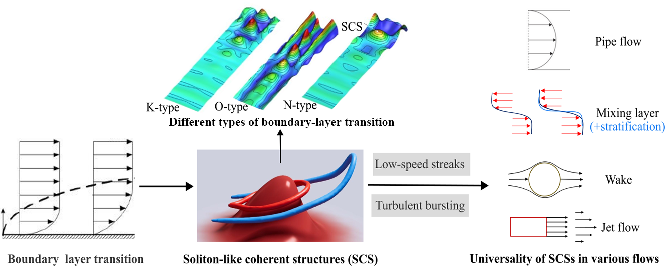
The formation, evolution, and dynamics of flow structures in wall-bounded turbulence have long been central themes in fluid-mechanics research. Over the past three decades, Soliton-like Coherent Structures (SCSs) have emerged as a ubiquitous and unifying feature across a wide range of shear flows, including K-type, O-type, N-type, and bypass transitional boundary layers, as well as fully developed turbulent boundary layers, mixing layers, and pipe flows. This paper presents a systematic review of the fundamental properties of SCSs and highlights their fundamental role in multiple transition scenarios. The analysis further explores the connection between SCSs and low-speed streaks, offering insight into their coupled dynamics. The phenomenon of turbulent bursting is also examined within the context of SCS dynamics. Together, these studies underscore the potential of SCSs to serve as a coherent dynamical framework for understanding turbulence generation mechanisms in wall-bounded flows. Finally, the review extends to the manifestation of SCSs in other canonical flows, including mixing layers, stratified shear flows, and jets, confirming their universality and significance in fluid dynamics. These findings not only advance our understanding of turbulence generation but also offer a promising theoretical foundation for future research in transitional and turbulent flows.Graphic Abstract
Keywords
Since Reynolds’s pipe experiment showed that flow states can be categorized as either laminar or turbulent [1], the transition from laminar to turbulent flow has been an active field of research. Research on the laminar-to-turbulent transition problem has spanned over a century. During this period, numerous theoretical frameworks have been developed, including receptivity theory [2,3,4], linear stability theory [5,6], weakly nonlinear theory [7], secondary instability theory [8], three-wave resonance theory [9], and transient growth theory [10]. These theoretical advances have significantly deepened our understanding of the transition process, yet critical gaps remain in explaining the nonlinear stage and laminar breakdown mechanisms.
Beyond theoretical approaches, many researchers have sought to identify the fundamental coherent structures that dominate the transition. Extensive experimental and computational studies have revealed a rich variety of flow structures in wall-bounded flows, such as Λ-vortices [11], soliton-like coherent structures (SCSs) [12], hairpin vortices [13], high-speed and low-speed streaks [14,15,16,17], streamwise vortices [18], chain of ring vortices [19,20,21,22], and turbulent spots [23,24,25,26,27]. These differ greatly in morphology, scale, and generation mechanisms, and no consensus exists on which dominates turbulence production. Over the past two decades, advances in direct numerical simulation (DNS) and tomographic particle image velocimetry (Tomo-PIV) techniques have enabled an increasingly detailed characterization of these flow structures and their dynamic evolution, offering new opportunities to unravel the underlying physics of transition. Lee and Wu [28], as well as Lee and Jiang [29], have systematically summarized and discussed the flow structures in wall-bounded flows. Since 2020, significant progress has been made in the study of SCS in wall-bounded flows. SCSs have been found to play a crucial role in the generation of turbulence in various wall-bounded flows, including K-type, O-type, N-type, and bypass transitional boundary layers, turbulent boundary layers, mixing flow, and pipe flow.
Unlike previous review articles, this paper specifically focuses on SCSs in wall-bounded flows and aims to elucidate the crucial role of SCSs in turbulence generation. The organization of this work is as follows: Section 3 systematically presents the discovery, formation mechanisms, and key characteristics of SCSs; Section 4 discusses the SCSs in K-type, N-type, O-type, and bypass transition; Section 5 explores the formation of low-speed streaks in the boundary layer and their relationship with SCS; Section 6 discusses the nature of turbulent bursting; Section 7 discusses SCSs in pipe flow; Section 8 primarily discusses the SCS discovered in various flows, demonstrating the universality of such structures in fluid motion; The conclusions are given in Section 9.
2 Experimental Techniques and Data Processing
Flow visualization is one of the most intuitive and effective methods for studying the transition process from laminar to turbulent flow. In the past, numerous studies have obtained extensive images of flow structures in wall-bounded flows through various flow visualization techniques. These intuitive visualization results have significantly enriched our understanding of wall-bounded flows. The famous Reynolds pipe experiment clearly demonstrated both laminar and turbulent flow states in pipe flow using dye injection visualization. The hydrogen bubble flow visualization technique is one of the most common flow visualization methods. Hama et al. [11] clearly showed the Λ vortex in a transition boundary layer using hydrogen bubble visualization. Although hydrogen bubble visualization is primarily used for qualitative observation of flow structures, certain velocity field information can also be extracted by processing hydrogen bubble timeline images [30,31,32,33]. Traditional flow visualization methods are typically limited to a single perspective, providing relatively limited flow field information. To overcome this limitation, some researchers [31,34,35] attempted to combine images captured simultaneously from two different perspectives to obtain more comprehensive flow field information. However, traditional flow visualization methods still face challenges in quantitatively capturing transient, three-dimensional structural evolution processes.
With the rapid development of experimental techniques, it is now possible to analyse the coherent structures of flow fields with high spatio-temporal resolution using Tomo-PIV [36,37,38] or particle tracking velocimetry [39,40]. For instance, Elsinga et al. [41] employed Tomo-PIV to study turbulent boundary layers at Reynolds number Re = 1900, focusing on the logarithmic and wake regions, and examined the relationship between turbulent bursts and vortex structures. Similarly, Lin et al. [42], Dennis and Nickels [43], Tang et al. [44], and Gao et al. [45] utilized stereo particle image velocimetry (SPIV) or Tomo-PIV to investigate transient behaviors in the logarithmic region of turbulent boundary layers. Additionally, based on time-resolved Tomo-PIV techniques, Schroder et al. [46] explored flow structures in turbulent boundary layers at different Reynolds numbers. These studies primarily adopted Eulerian perspective methods and employed iso-surface approaches to characterize transient flow structures. However, due to limitations of conventional flow visualization techniques, wave structures in the near-wall region remain challenging to identify accurately. As noted by Lee [28], reconstructing three-dimensional flow structures and their evolution processes remains a critical problem in fluid mechanics. Recently, Jiang et al. [47,48,49] conducted research on low-speed streak structures in transitional and turbulent boundary layers using Lagrangian particle tracking methods (timelines and material surfaces). By reconstructing flow structures based on three-dimensional velocity fields obtained through Tomo-PIV and nonlinear parabolized stability equations (NPSE), they clearly revealed the flow evolution process and successfully observed the vortex generation mechanism induced by SCS. This method provides a powerful tool for studying the evolution of SCS. Tomo-PIV and NPSE provide three-dimensional velocity field with spatiotemporal resolution. The key to capturing the dynamics of SCS lies in combining the Lagrangian analysis method (developed by Jiang et al. [48]) and the Eulerian analysis method. The Lagrange method (such as timelines, material surfaces) can clearly show SCSs. Combined with the display of surrounding vorticity, the development of vortices during the SCS development process can be clarified, thereby showing the dynamic process of SCS.
In 1998, Lee [12] investigated the nonlinear stage of K-type transition and discovered a coherent structure, which behaves like a soliton. Fig. 1 shows SCS visualized using parallel hydrogen bubble lines, where it appears as a bulge. Fig. 2 shows the plan view of the SCSs, with the K marking the SCSs in the diagram. The Fig. 1 shows that the SCS gradually moves away from the wall, while the surrounding fluid moves toward the wall, leading to the formation of a shear layer. Lee pointed out that the lifting of the SCS and the downward sweeping of the surrounding fluid are key mechanisms for vortex generation. Lee proposed that SCSs are typically localized three-dimensional waves.
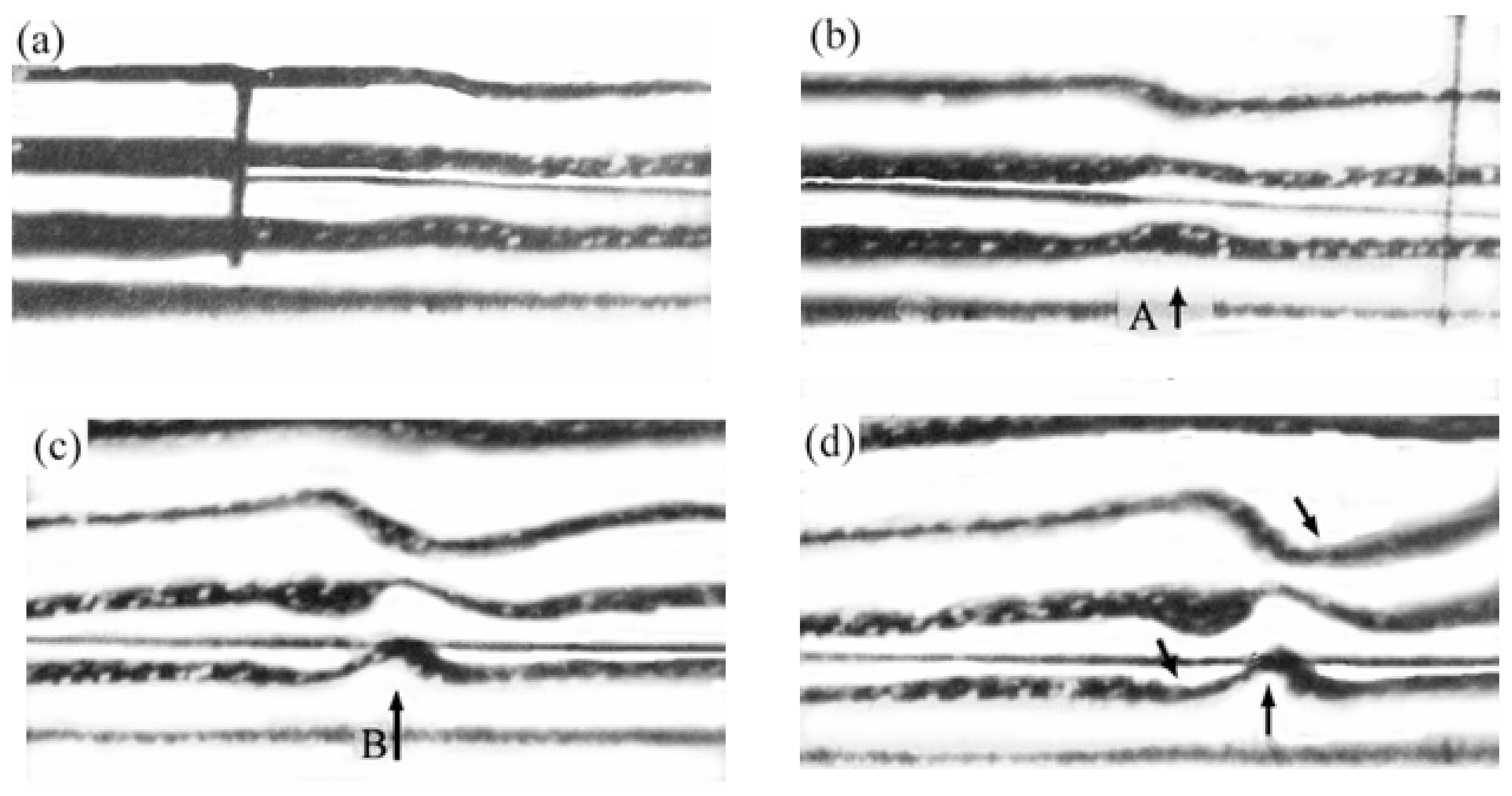
Figure 1: Side view of SCS in K-type transition. (a–d): t = 0, 0.66, 1, 1.3 s. Reproduced with permission from Lee [12]. Copyright 1998 Published by Elsevier B.V.
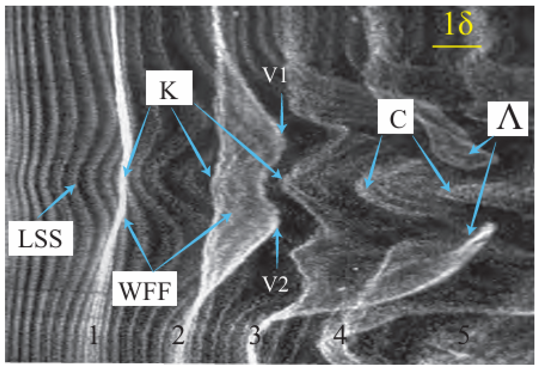
Figure 2: Plan view of SCS in K-type transition. Reprinted with permission from Jiang et al. [48]. LSS: low-speed streak; K: kink-like pattern; WWF: warped wave front; C: chevron-like patterns. The two wings or ‘valleys’, labelled V1 and V2, pass over the timelines of the LSS and quickly surround the kink-like structure to form a Λ-vortex (labelled as Λ). Copyright 2020 Cambridge University Press.
In 2000, Lee [19] further investigated the characteristics of flow structures in a K-type transitional boundary layer. Lee pointed out that the SCS is generated through the nonlinear interaction of two oblique waves with the same frequency but opposite spanwise wave angles. Recent work by Yang et al. [50] confirmed the presence of oblique waves upstream and downstream of the flat plate leading edge, providing strong support for the generation of SCS through oblique wave interactions (Fig. 3). In the late stage of K-type transition, Lee observed various flow structures, including SCSs, low-speed streaks, hairpin vortices, and chain of ring vortices. Based on the SCS, Lee proposed a possible universal transitional scenario.
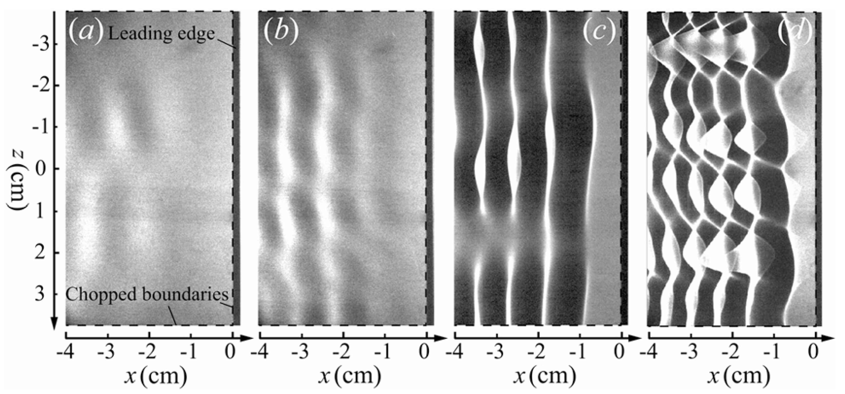
Figure 3: Oblique waves upstream of the leading edge of the plate visualized by the refraction method. Leading edge is at the right end of each panel. (a–d): t = 0.14, 0.16, 0.18, and 0.20 m/s. Reprinted with permission from Yang et al. [50]. Copyright 2023 AIP Publishing.
Subsequent experimental studies by Lee [20] further revealed that the spike phenomena observed in the velocity time series were induced by chain of ring vortices. The experimental results demonstrated that the formation of these chain of ring vortices originates from the interaction mechanism between Λ vortices and secondary vortex rings.
In 2001, Lee and Li [51] used hydrogen bubble flow display and two-dimensional hot film measurement techniques to analyse the dynamic relationships between solitaire waves and Λ vortices, as well as secondary closed vortex (SCV) and low-speed streaks. Fig. 4 (further documented in Lee and Chen [52]) shows the evolution process of SCS and Λ vortices, with a time interval of 1/12 s between consecutive frames. It can be clearly observed that the SCS initially manifests as a kink-like structure, followed by the gradual formation of Λ vortices around it. This temporal sequence demonstrates that the formation of SCS precedes the generation of Λ vortices.
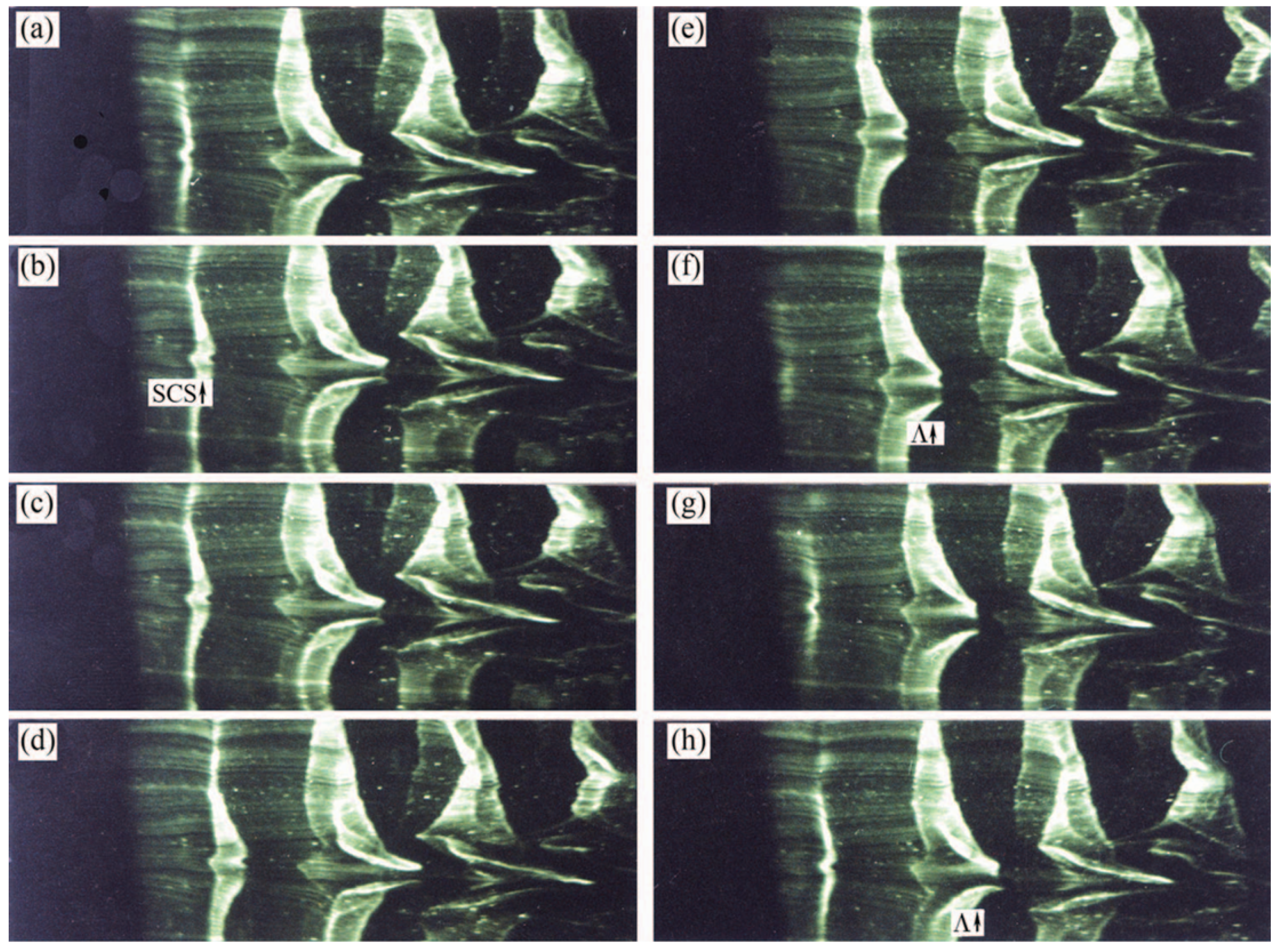
Figure 4: Hydrogen bubbles visualization of SCS and Λ vortex. The wire was located parallel to the plate and normal to the flow direction with the flow from left to right. The wire was positioned at y = 0.75 mm. The time interval between successive figures was 1/12 s. (a–d): show the development of the SCS (see the arrow labeled SCS); (e–h): shows the formation of the Λ-vortex (see the arrow labeled Λ). Reprinted with permission from Lee and Li [51]. Copyright 2001 Published by Elsevier Ltd.
Fig. 5 shows the SCS and the secondary closed vortex around SCS. Lee and Li [53] showed that the formation of these secondary closed vortices results from the high-shear layers created by lifting the SCS and the downward movement of the surrounding fluid. Lee and Li pointed out that the interaction between secondary closed vortex rings and Λ vortices serves as the fundamental mechanism for generating high-frequency vortices (chain of ring vortices).
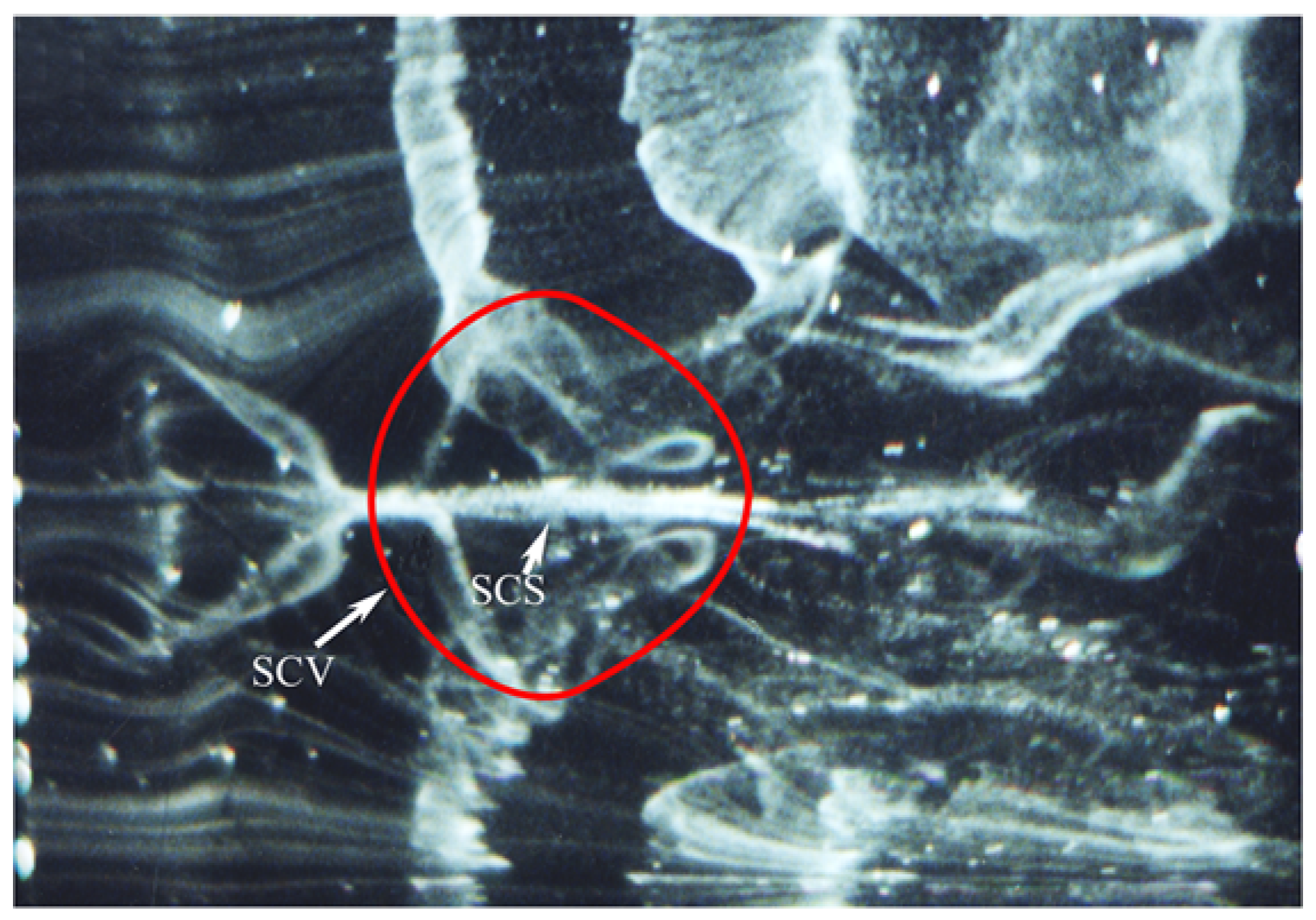
Figure 5: Hydrogen bubbles visualization of SCS and secondary closed vortex (SCV). Reprinted with permission from Lee and Wu [28]. Copyright 2008 American Society of Mechanical Engineers.
Based on a series of experimental observations by Lee, the SCS exhibits the following characteristic features:
- 1.SCS is a localized three-dimensional wave structure generated through the nonlinear interaction of a pair of oblique waves with the same frequency but opposite wave angles;
- 2.SCS propagates downstream at 0.6–0.8U∞ (where U∞ is the freestream velocity) while exhibiting an upward lifting motion at approximately 0.1U∞; the propagation of SCS enhances near-wall velocity, resulting in increased skin friction.
- 3.SCS maintains near-constant amplitude during downstream evolution and has a significantly longer life cycle than other transitional structures.
It is necessary to distinguish between the SCSs and the coherent structures/solitons (CS-Solitons) discovered by Borodulin and Kachanov [54]. They first identified the soliton-like nature of spike signals. These spikes quickly lift from the wall and propagate downstream at freestream velocity along the boundary layer’s outer edge, with slowly decaying amplitude. The traces of this soliton property were visualized for x = 400 to 600, and the soliton was observed to travel downstream almost along the line of y = δ which is constant. The local mean flow velocity in the point where the soliton is positioned approaches freestream velocity, with its amplitude width varying slowly. They named these structures as coherent structures/solitons (CS-Solitons). Subsequent research revealed that these spike signals are caused by ring-like vortices in the late stages of transition. Kachanov et al. [21] further pointed out that the localization of high-frequency disturbances in the late transition stages ultimately leads to the formation of CS-Solitons. The study by Bake et al. [55,56] demonstrated that the multiple reconnections of the vortex legs near the heads of Λ vortices are the direct mechanism for the generation of ring-like vortices (i.e., CS-Solitons). Kachanov argued that CS-Solitons are high-frequency structures relative to Λ vortices. In 1998, Lee [12] used the term CS-Solitons to describe localized three-dimensional wave structures in K-type transition. This was because when Lee et al. observed three-dimensional waves during the early natural transition experiments, they assumed, perhaps too simplistically, that they had visualized Kachanov’s CS-solitons and failed to fully grasp their depth. However, Borodulin et al. [57] argued that CS-Solitons are chain of ring vortices, not the SCS discovered by Lee. Fig. 6 shows the chain of ring vortices (i.e., CS-Solitons) experimentally observed by Borodulin et al. Subsequent growing experimental and computational evidences suggest that it is the SCS that dominates the turbulence generation.
Figure 6: Three spikes induced by ring-like vortices (i.e., CS-Solitons) in the late stage of K-type transition. Reprinted with permission from Borodulin et al. [57]. Copyright 1969 Springer-Verlag Berlin Heidelberg.
Lee and Li [53] later introduced the term SCS to describe the localized three-dimensional wave structures in the transitional boundary layer. Lee [19] showed that SCS is a localized three-dimensional wave generated by the interaction of a pair of oblique waves, persisting from the early to late stages of transition (x < 260 mm versus x ≈ 500 mm in Kachanov’s observation). In 2008, Lee and Wu [28] further clarified that SCS itself is not a high-frequency structure; rather, it is the secondary vortex rings produced by SCS that interact with Λ vortices to form high-frequency vortex structures (such as chain of ring vortices). The differences between SCS discovered by Lee and CS-Solitons discovered by Kachanov are summarized in Table 1.
Table 1: Comparison of CS-solitons and SCS characteristics.
| Characteristic | CS-Solitons Proposed by Kachanov | SCS Discovered by Lee |
|---|---|---|
| Type | Vortical structures characterized as chains of ring vortices | Localized three-dimensional waves |
| Developing stage | Downstream of Λ-vortex | Precedes Λ-vortex initiation |
| Spatial scale | Entire boundary layer | Entire boundary layer |
| Formation Mechanism | Formed through stretching and reconnection of Λ-vortices | Generated by the interaction of two oblique waves |
| Frequency | High-frequency structures, typically four times of Λ-vortex frequencies | Shares the frequency of Tollmien-Schlichting (T-S) waves or Λ-vortices |
| Velocity | Approach free-stream velocity | 0.6–0.8 free-stream velocity |
| Lifetime | More than 4 times the T-S wave period | More than 7 times the T-S wave period |
We provide a detailed discussion of their key differences. The spike-soliton concept proposed by Kachanov is closely related to his wave-resonant theory, which describes the resonant amplification of harmonic disturbances within the boundary layer. This theoretical framework is fundamentally important for understanding both the evolution of the frequency-wavelength spectrum and the K-type breakdown process in near-wall turbulence. The CS-soliton exhibits an interaction with turbulent background noise, leading to parametric resonant amplification of random fluctuations—an effect that has been characterized as having a catalytic influence on the transition process [21]. This phenomenon likely occurs because the CS-soliton appears in the late transitional stage within the upper boundary layer, where it facilitates energy transfer from the mean flow and ultimately triggers flow breakdown.
The SCS shares with the CS-soliton the characteristic property of minimal dispersion in both spatial and temporal domains. However, the SCS emerges significantly upstream of Λ-vortex formation, the typical vortical structure in transitional boundary layers. Comprehensive timeline analyses—including both experimental visualizations using hydrogen bubble techniques ([28,53]) and numerical simulations employing NPSE and Tomographic PIV methods ([48,49])—clearly reveal the three-dimensional geometry of the SCS as it develops from the near-wall region to the boundary layer edge. These observations confirm that the SCS spans the entire boundary layer thickness and appears during the very early stages of transition. In contrast, the CS-soliton demonstrates markedly different behavior, growing rapidly from the near-wall region to the boundary layer edge while maintaining a consistent vertical (y) position in the downstream direction. This distinct growth pattern suggests fundamentally different underlying dynamics between these two structures, particularly in their relationship to Λ-vortex formation.
The SCS serves as the primary initiator of Λ-vortex formation through processes of wave amplification and three-dimensional warping (resulting from SCS instability), while the CS-soliton represents a later-stage phenomenon that emerges from the interaction between a Λ-vortex and a secondary closed vortex structure (which itself originates from secondary instability of the SCS) [28]. At the boundary layer edge, the SCS maintains a persistent wavefront with frequency characteristics identical to those of Tollmien-Schlichting waves or Λ-vortices, as demonstrated in [48]. This frequency signature differs notably from the high-frequency structures detected by Borodulin et al. [57] using hot-wire anemometry (see Fig. 6). Additional evidence of their distinct behaviors comes from propagation velocity measurements: the SCS moves at 0.6 to 0.8 times the freestream velocity, while the CS-soliton approaches the freestream velocity. These velocity differences have measurable consequences—the relatively faster near-wall motion of the SCS produces characteristic tooth-shaped jumps in velocity profiles (visible in oscilloscope traces), while its slower motion near the boundary layer edge generates distinctive spike patterns during early transitional stages. The typical lifetime of the SCS exceeds that of the CS-soliton, lasting over seven times the T-S wave period for SCS compared to four times the T-S wave period for CS-soliton, as reported in [53].
In summary, the key differences between CS-solitons and SCSs lie in their fundamental nature (vortices vs. waves), formation origins (Λ-vortices vs. oblique waves), and frequency characteristics. CS-solitons exhibit multiples of Λ-vortex frequencies, while SCSs share the same frequency as T-S waves and Λ-vortices.
Based on the descriptions provided in this section, the key flow structures are summarized in Table 2 to enhance readability and provide a clear reference for the subsequent sections.
Table 2: Definitions of key flow structures in wall-bounded and shear flows.
| Structure | Definition |
|---|---|
| Soliton-like Coherent Structure (SCS) | Localized 3D wave structures formed by oblique wave interactions, triggering Λ-vortex formation. |
| Λ-vortex | Λ-shaped vortices arising from stretched vortex lines, acting as precursors to hairpin vortices due to SCS stability. |
| Secondary Closed Vortex (SCV) | Vortical loops generated by high-shear layers around SCSs, resulting from secondary SCS instability. |
| CS-Soliton | High-frequency chain of ring vortices in late transition, created by interactions between Λ-vortices and secondary closed vortices. |
| Chain of Ring Vortices | High-frequency ring-shaped vortices in chains, same as CS-Soliton, developing from Λ-vortex reconnections, leading to velocity spikes in late transition. |
| Low-Speed Streak (LSS) | Elongated low-momentum fluid regions near the wall in boundary layers formed by SCS sequences and tied to turbulence bursts. |
| Turbulent Spot | Localized turbulent patches in transitional flows, composed of SCSs, vortices, and streaks, expanding into an arrowhead shape to achieve full turbulence. |
4 SCSs in K-Type, N-Type, O-Type, Bypass Transition
There are four widely accepted transition paths for boundary layer transition: (1) K-type; (2) N-type; (3) O-type; and (4) bypass transition. Among these, the K-type transition is caused by the nonlinear interaction between a two-dimensional plane wave (ω1, 0) and a pair of oblique waves with the same frequency but opposite wave angles (ω1, ±β). This type of transition was first observed by Klebanoff et al. [58] in controlled experiments. The flow field evolution of K-type transition exhibits the following typical characteristics [56]: First, the development of three-dimensional oblique waves modulates the base flow field, causing the fluctuating velocity to exhibit a spanwise non-uniform distribution, forming peak and valley regions. Subsequently, the flow structures evolve into streamwise aligned Λ-vortices. In the later stages, the legs of the Λ-vortices undergo multiple reconnection to form ring-like vortices, while high-frequency disturbances appear in the velocity time series, manifesting as spikes.
The N-type transition is triggered by the nonlinear interaction between a two-dimensional fundamental plane wave (ω1, 0) and a pair of oblique waves with half the fundamental frequency but opposite wave angles (
The O-type transition is a transition process initiated by the nonlinear interaction between a pair of oblique waves with identical frequency but opposite wave angles (ω1, ±β). Goldstein et al. [59] first investigated this nonlinear interaction mechanism between oblique waves in a two-dimensional shear layer. During this transition process, the nonlinear interaction of oblique waves initially generates streamwise vortex structures. These streamwise vortices then significantly modulate the base flow field, ultimately leading to the formation of periodically spanwise-distributed high- and low-speed streaks with large amplitudes [60].
Although K-, N-, and O-type transitions differ in their initial conditions and nonlinear interaction mechanisms, studies have shown that these three transition modes exhibit high similarity in their late-stage evolution. All three transitions develop Λ-structures and display spike and multiple-spike characteristics in the velocity time series [61,62]. Berlin et al. [61] pointed out that these transitions ultimately manifest as interactions between three-dimensional oblique waves and streamwise vortices. While investigating K-type transition, Lee et al. [12] discovered SCS and used the SCS concept to explain the formation of hairpin vortices and chain of ring vortices during the late stages of boundary layer transition, thereby proposing a universal transition mechanism centered on SCS. Chen [63] used DNS to study the process of vortex structure generation in a transitional boundary layer and confirmed that SCS structures play a key role in vortex formation.
Recently, Jiang et al. [48] conducted systematic studies on K-, N-, and O-type transitions using NPSE. Their results demonstrate that different transition paths share similar evolutionary characteristics: in their late stages, the material surfaces all exhibit SCS. Fig. 7 shows that the lifting of the SCS, combined with the downwash of the surrounding fluid, forming longitudinal valleys (V) flanking the sides of the SCS and depression regions (S) at the bottom of the wave front. This process is considered the key mechanism for hairpin vortex generation. Jiang et al. [49] further demonstrated that SCS plays a crucial role in generating vortical structures during the K-type transition under an adverse pressure gradient and in the formation of turbulent spots in a compressible boundary layer.
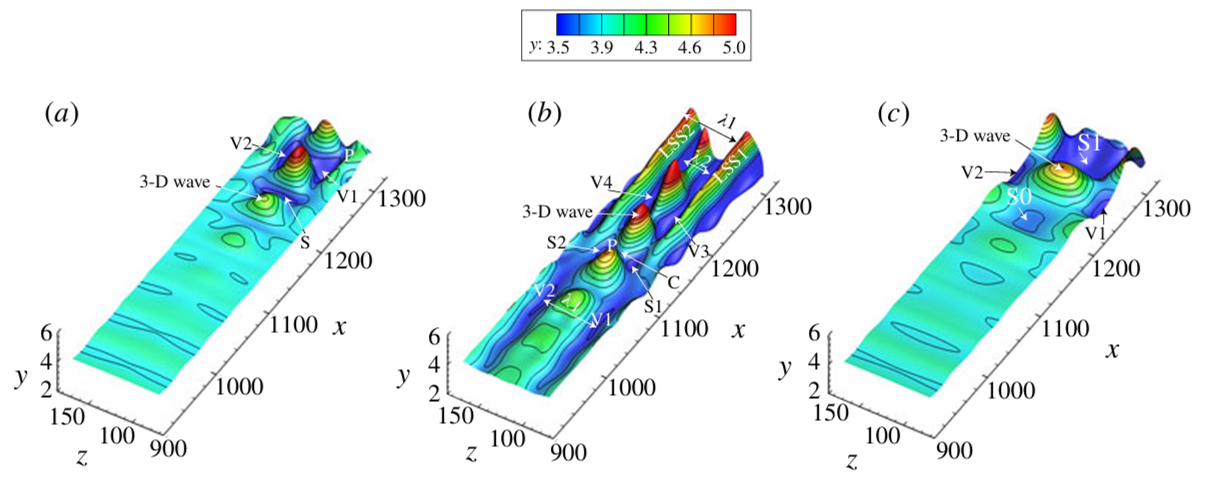
Figure 7: Deformation of material surfaces: (a) K-regime transition; (b) O-regime transition; (c) N-regime transition. Reprinted with permission from Jiang et al. [48]. Copyright 2020 Cambridge University Press. S for depression region; V for valley; LSS for low-speed streaks; P for crest of the 3D wave; C for chevron-shape pattern; λ is the spacing between the valleys.
Hu et al. [64,65] investigated the evolution of turbulent spots in a flat plate boundary layer using Tomo-PIV and DNS. The results of both experimental and DNS demonstrate that SCSs play a crucial role in the development of turbulent spots. As the turbulent spot evolves downstream, low-speed streaks gradually form at its edges, exhibiting the behavioral characteristics of SCS. With the uplift of SCS, the surrounding fluid moves towards the wall surface, resulting in the accumulation of vortices at the boundary of SCS. This process generates high-shear layers at the interfaces of the waves. These high-shear layers subsequently roll up to vortical structures. The findings of Hu et al. confirm that SCSs are key to vortex generation within turbulent spots and play a significant role in their evolution. Fig. 8 presents the deformation of a material surface released in the near wall region from DNS by Hu et al. The material surface exhibits lifted streamwise streaks, which consist of several SCSs. This observation suggests that a turbulent spot is a complex flow structure composed of SCSs and vortices induced by SCSs.
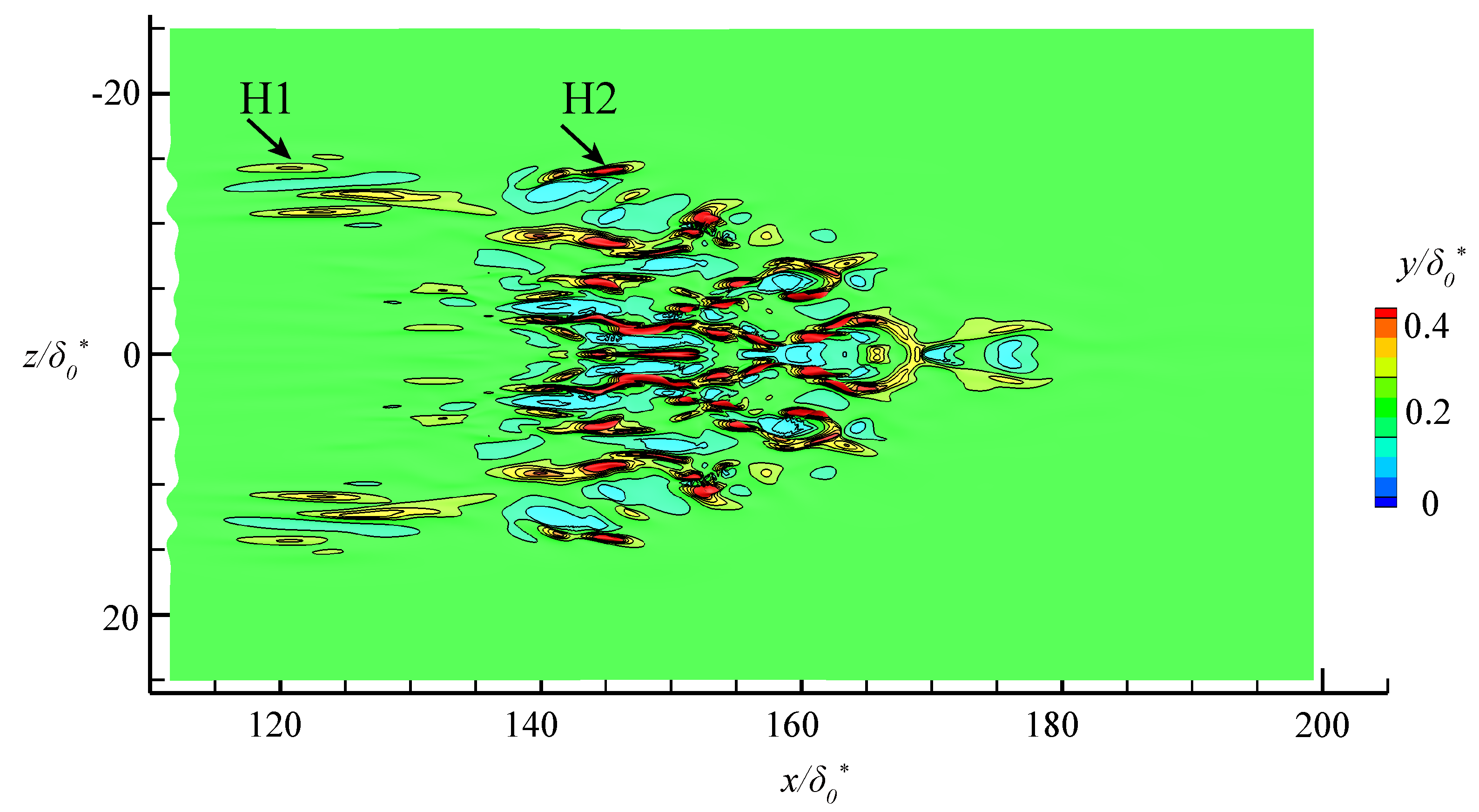
Figure 8: SCSs in turbulent spots. H1: Early stage low-speed structure; H2: Low-speed streak consisting of SCSs.
From a historical perspective, the discovery of the SCS-driven transition scenario builds upon foundational work on the K-type boundary-layer transition. This development incorporates two key classical findings: (1) the traditional transition process involving Tollmien-Schlichting wave amplification and three-dimensionalization, Λ-vortex formation through wave resonance, and turbulent spot formation and coalescence into full turbulence [11,58]; and (2) Kachanov’s controlled transition scenario featuring formation of a chain of ring vortices through Λ-vortex leg reconnection, which occurs without turbulent spot development [21,55,56,57].
To enhance the understanding of the previous transition, the SCS-based transition framework offers novel insights into the boundary-layer transition process, which follows this sequence:
- 1.SCS formation through oblique wave interactions;
- 2.Λ-vortex generation via SCS instability;
- 3.Secondary closed vortex (SCV) formation from SCS secondary instability;
- 4.A chain of ring vortices and two streamwise vortices production through Λ-vortex/SCV interaction, with associated near-wall streaks formation;
- 5.Turbulence onset through breakdown of ring vortices due to their dynamic interaction with SCS.
The SCS framework elucidates the mechanism of vortex formation and their interrelationships. Certain transition types involve only a subset of these stages, while others give rise to more complex synthesized structures, such as low-speed streaks and turbulent spots. The SCS plays a central role in the transition process, significantly advancing the framework for the origin of wall-bounded turbulence.
5 Formation of Low-Speed Streaks
Low-speed streaks are ubiquitous in transitional and turbulent boundary layers. Due to their close association with bursting events and turbulence production, they have attracted extensive attention from researchers. Since the experiments by Runstadler and Kline [66] in the 1960s, the study of low-speed streaks has spanned nearly six decades, yet controversies remain regarding their formation mechanisms. Low-speed streaks do not rotate and are therefore not vortex structures. In turbulent boundary layers, they exist primarily in the buffer layer and in the near-wall region of the logarithmic layer, with a normalized spanwise spacing of approximately z+ ≈ 100. Recent studies have found that the normalized spacing of low-speed streaks becomes Reynolds number independent in the outer logarithmic region as the distance from the wall increases [67]. Low-speed streaks in transitional boundary layers differ from those in turbulent boundary layers, a distinction first discussed by Kline et al., who termed them transition streaks and wall-layer streaks, respectively [14].
Some researchers regard low-speed streaks as autonomous flow structures capable of generating other coherent structures (e.g., hairpin vortices and streamwise vortices), whereas others consider them merely as byproducts of such structures. Most studies based on hairpin vortices support the second view, suggesting that low-speed streaks are the result of the uplift of low-momentum fluid induced by the legs and head of hairpin vortices [68,69] or constitute part of uniform momentum zones induced by hairpin vortex packets.
However, an alternative viewpoint argues that low-speed streaks can form without vortex induction. Landahl’s [70,71] linear inviscid model demonstrates that low-speed streaks can emerge from any initial three-dimensional perturbation as long as it has nonzero net momentum in the wall-normal direction. Such perturbations may originate from local three-dimensional inflectional instabilities with spanwise asymmetry (e.g., oblique wave perturbations). Studies show that removing the term v(∂U/∂y) (where v is the wall-normal fluctuating velocity and U is the mean streamwise velocity) from the Navier-Stokes equations prevents the formation of low-speed streaks, highlighting the critical role of wall-normal fluctuations and supporting Landahl’s theory [72]. Furthermore, Chernyshenko and Baig [73] proposed that low-speed streaks arise from the combined effects of three mechanisms without requiring hairpin vortex induction: (1) uplift of low-speed fluid, (2) perturbation amplification in shear layers, and (3) viscous diffusion.
In the study of K-type transition, Lee and Li [53] utilized hydrogen bubble visualization to observe low-speed streaks in the near-wall region during the late stages of transition, revealing that these streaks are not singular structures but rather composites consisting of multiple SCS. Lee and Wu [28] further discussed the streamwise alignment of multiple SCS, elucidating their role in the formation of low-speed streaks. Recently, Jiang et al. [48] systematically investigated transition paths in the K-regime, N-regime, and O-regime using NPSE. Fig. 7 illustrates the characteristics of material surfaces in the late stages of different transition paths obtained from their study. The results demonstrate that, despite the differences in transition paths, they all exhibit a significant common feature in the late stages: the material surface displays a series of raised SCS structures, accompanied by the formation of depression regions and longitudinal valleys. Their further analysis revealed that the low-speed streaks in the transitional boundary layer are closely associated with inflection regions in the normal timelines and lagging regions in the time-line surfaces. These behaviors of the timelines are actually caused by the amplification of SCSs. Therefore, the low-speed streaks can be regarded as a spatial combination of multiple consecutive SCS structures in the streamwise direction. This concept, through a comparison between schematic diagrams and experimental images, is illustrated in Fig. 9. Fig. 9a shows the flow visualization of near-wall low-speed streaks obtained by Lee and Li [53] using hydrogen bubbles; Fig. 9b presents a conceptual side-view model of the corresponding low-speed streaks; Fig. 9c,d depict top-view characteristics at different height cross-sections. As shown in Fig. 9c, at the lower height (Level 1), the cross-section shows no clear boundaries between the three SCS, appearing as a continuous integrated structure. In contrast, at the higher height (Level 2) in Fig. 9d, the SCS structures manifest as isolated units, clearly indicating that the low-speed streaks are composed of multiple discrete SCS.
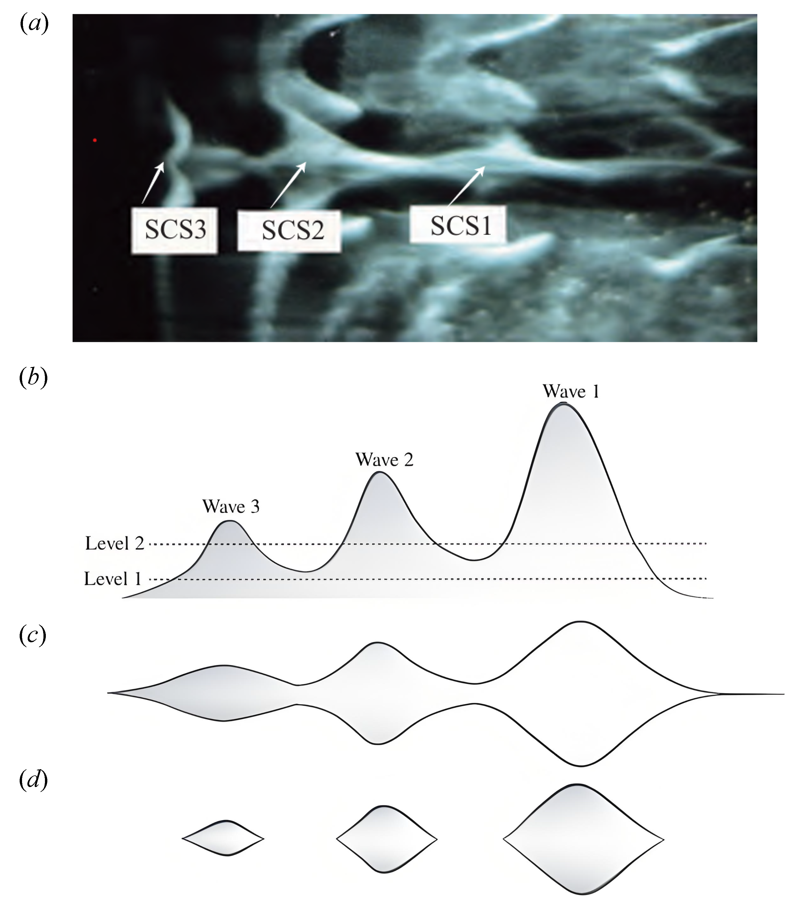
Figure 9: Low-speed streak in transitional boundary layer: (a) hydrogen bubble visualization of low-speed streak at the near-wall region [53]; (b) side view of low-speed streak consisting three localized 3D waves [48]; (c) plan view of low-speed streak at level 1 [48]; (d) plan view of low-speed streak at level 2 [48]. (a) reproduced with permission from Lee and Li [53]. Copyright 2008 American Society of Mechanical Engineers. (b–d) reproduced with permission from Jiang et al. [48]. Copyright 2020 Cambridge University Press.
Elofsson [74] investigated the oblique wave transition induced by a pair of oblique waves in a flat-plate boundary layer, and the corresponding flow visualization images are presented in Fig. 10. Although Elofsson suggested that the late stage of oblique wave transition is triggered by the secondary instability of low-speed streaks leading to turbulence, Fig. 10 clearly shows the emergence of SCSs already in the early transition stage. These SCS align in the streamwise direction, forming low-speed streaks. In fact, the secondary instability of low-speed streaks is essentially caused by the destabilization of the high-shear layers that develop at the boundaries of the amplified SCS. Eventually, the instability of these shear layers leads to their roll-up, forming hairpin vortices. Fig. 11 displays the low-speed streaks and vortices in K-type transition obtained by Lee and Wu [28] using hydrogen bubble visualization. As shown in the Fig. 11, the hydrogen bubbles aggregate into an elongated streak, which is the result of multiple SCSs and vortices induced by SCSs. This phenomenon shows similarity to the low-speed streak breakdown process illustrated by Elofsson in Fig. 10.
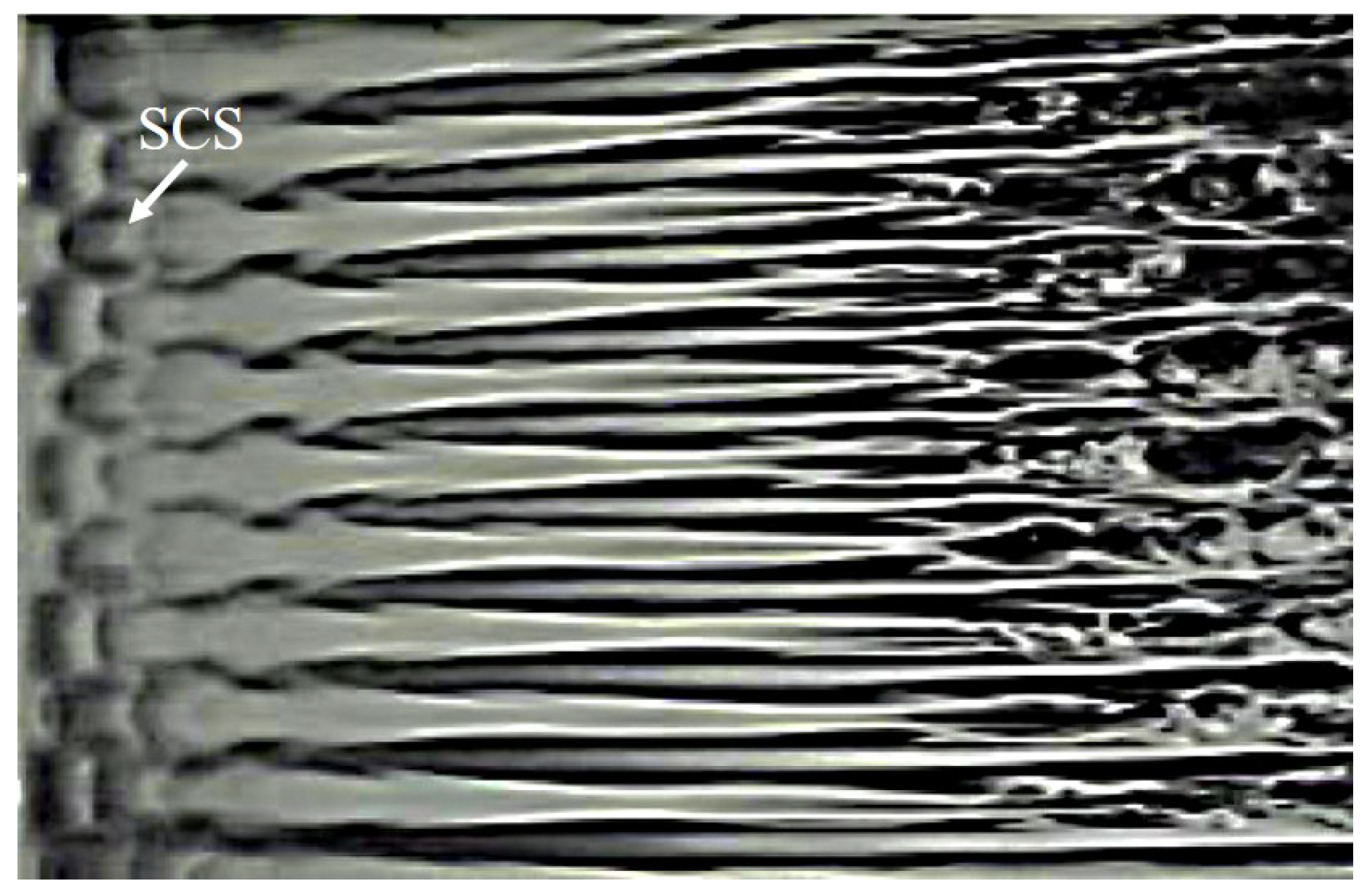
Figure 10: Visualization of streaks in an oblique transition in a Blasius flow. SCS appears at early stage due to the interaction of oblique waves. Reprinted with permission from Elofsson [74].
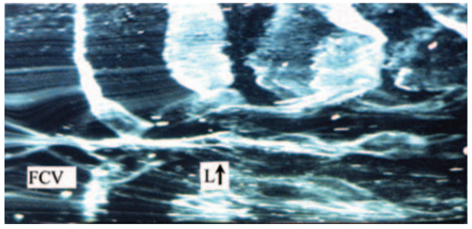
Figure 11: Flow visualization of K-type transition in a Blasius flow [28]. FCV: first closed vortex; L: low-speed streaks. Reprinted with permission from Lee and Wu [28]. Copyright 2008 American Society of Mechanical Engineers.
6 The Nature of Turbulent Bursting
Runstadler et al. [66] were the first to use the term “bursting” to describe the phenomenon of turbulence production in turbulent boundary layers. Kline et al. [14] further conducted detailed studies on low-speed streaks in turbulent boundary layers. Their research revealed that low-speed streaks exist in the region very near the wall. The lifting of these low-speed streaks and their interaction with outer-layer fluids lead to oscillation, bursting, and ejection of the streaks. Kim and Kline et al. [15] further investigated the relationship between turbulence production and bursting. Their studies showed that in the region 0 < y+ < 100, almost all turbulent kinetic energy is generated during bursting, primarily during the oscillation growth stage. They divide the bursting event into three stages:
- 1.The lifting of low-speed streaks from the region very close to the wall, resulting in an inflection point in the velocity profile;
- 2.The instability of the inflection region leading to rapid growth of disturbances;
- 3.The breakdown of the oscillatory, ordered structure into chaotic, turbulence.
Offen and Kline et al. [16] proposed a model for bursting in turbulent boundary layers. In this model, wall streaks are regarded as a sublayer of the boundary layer, and the lifting of streaks may be caused by local adverse pressure gradients due to upstream bursting sweep events or outer-layer vortex structures. Although the definition of the term “bursting” remains somewhat ambiguous, it is always closely associated with the ejection of low-speed streaks and the sweep of high-speed fluid. Various techniques have been developed to detect ejections and sweeps. Rao et al. [75] used bandpass-filtered velocity signals to determine the period of bursting. Blackwelder and Kaplan [76] employed the variable interval time averaging technique to detect significant changes in the streamwise velocity profile.
Lee and Wu [28] pointed out that bursting is essentially caused by the behavior of SCS. Specifically, low-speed streak structures are composed of multiple SCSs, and several key phenomena during bursting are closely related to the behavior of SCSs. For example, the lifting of low-speed streaks results from the amplification and lifting of SCSs from the wall; the observed sweep of outer-layer fluid during bursting aligns with the downward motion of surrounding fluid during SCS lifting; and the subsequent breakdown during triggering resembles the vortex ring chain phenomenon induced by SCSs. Jiang et al. [47] used Tomo-PIV to study the behavior of low-speed streaks in turbulent boundary layers. Their results indicated that the lifting and oscillation of low-speed streaks, as well as the formation of initial vortices, can be explained by the amplification and breakdown of SCSs.
Recently, Jiménez [77] further demonstrated that long streaks are not a necessary condition for the self-sustaining process of turbulent bursting. Their study showed that bursting triggered by low-speed regions (essentially SCSs) with length scales comparable to the bursting scale is mechanistically no different from bursting generated by long low-speed streaks. Thus, the absence of long streak structures has minimal impact on turbulent bursting. This finding supports the idea that low-speed streaks are fundamentally composed of more basic SCS units. Turbulent bursting can be systematically described through the behavior of SCSs, providing a clearer and more complete physical picture. SCSs offer a unified framework for understanding the bursting process.
Based on the preceding discussion, we now revisit the framework of turbulent transition. The framework of traditional turbulent transition can be understood through disturbance magnitude dependence, as summarized by Morkovin et al. [78] in Fig. 12. For low disturbance conditions, natural transition progresses sequentially through boundary layer receptivity, modal linear growth, and nonlinear interactions leading to turbulent breakdown, with subclassifications (K-type, N-type including C-type and H-type variants, and O-type transition) depending on specific nonlinear interaction mechanisms. In contrast, high disturbance conditions induce bypass transition, where perturbations bypass the linear growth stage and proceed directly to nonlinear interactions. The discovery of SCSs provides a unifying framework that integrates previously distinct transition processes. Traditional transition pathways (as shown in Fig. 12a) primarily describe the growth of instabilities, tracing the process from the receptivity stage—where external disturbances enter the boundary layer–to the subsequent amplification, interaction, or bypass of these instability modes. In contrast, the transition process can be significantly simplified when adopting a structure-based perspective, which focuses on the evolution and interaction of coherent flow structures, as illustrated in Fig. 12b. The new framework reveals that: (1) receptivity fundamentally involves oblique wave interactions, and (2) the dynamical transition processes across various regimes can be unified through SCS dynamics and their induced vortical structures (Section 4). Previous studies extensively explored the vortex, but its origin remained unclear. The new wave-induced-vortex framework clearly demonstrates that localized 3D waves (i.e., SCS) trigger the formation of various vortices, driving the transition to turbulence. This revised paradigm (see also [29]) also naturally explains key turbulent features, as discussed in previous sections, including streaky structures and near-wall bursting behavior, as manifestations of SCS evolution, where SCSs directly form low-speed streaks (Section 5) and drive turbulent bursting events (Section 6). It is worth noting that the K-type boundary layer transition is specifically summarized in Fig. 12b, which clearly illustrates the distinction between the SCS and CS-soliton concepts (e.g., wave-dominated versus vortex-driven dynamics and different evolutionary stages), as also compared in Table 1. In the subsequent sections, we present the discovery of SCS and its driven transition processes in various shear flows beyond the boundary layer.
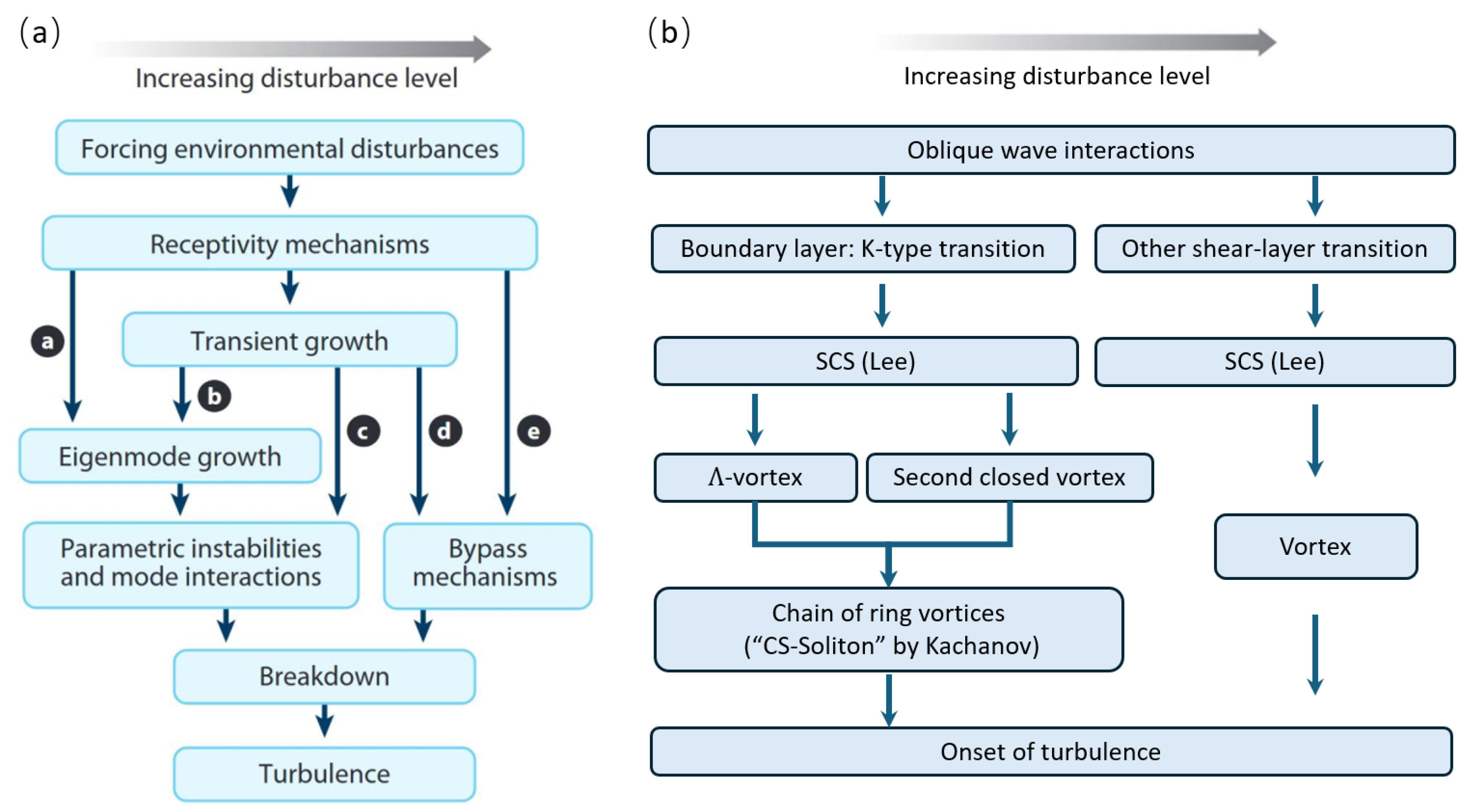
Figure 12: Transition to turbulence: (a) Boundary-layer flow, adapted from Morkovin et al. [78]. Copyright 1994 American Physical Society. (b) Updated transition path for general shear flows.
Since Reynolds’ pipe experiment in 1883, the transition problem in circular pipes has attracted widespread academic attention [79,80,81]. In experiments, the transitional Reynolds number for pipe flow typically occurs around 2000. However, the actual transition Reynolds number is highly dependent on the turbulence intensity of the incoming flow—when both turbulence intensity and flow disturbances are carefully controlled, transition can be significantly delayed. In a precisely controlled pipe flow experiment by Pfenniger [82], the transition Reynolds number was even extended to the order of 105.
Linear stability theory demonstrates that pipe flow remains stable for sufficiently small disturbances. Moreover, since the laminar velocity profile remains identical at different axial positions in pipe flow, its stability characteristics remain constant along the streamwise direction [83,84]. The onset of transition in pipe flow requires two simultaneous conditions: sufficiently high flow velocity and adequately strong disturbances. Regarding the observed intermittency phenomenon in pipe flow, the prevailing explanation suggests that when a sufficiently strong disturbance triggers local turbulence, the flow returns to laminar after the disturbance passes downstream, until encountering another sufficiently strong disturbance to reinitiate turbulence—this mechanism has been experimentally verified in multiple pipe flow studies.
The experiments by Hof et al. [79] demonstrated that as the Reynolds number increases, the threshold amplitude of disturbances required to trigger transition decreases. When the Reynolds number becomes sufficiently large, even very small perturbations can rapidly induce transition. Darbyshire et al. [83] conducted a series of experiments measuring the critical disturbance amplitudes for transition at different Reynolds numbers. Their key results are illustrated in Fig. 13, where circular markers indicate cases where the flow transitioned to turbulence, while square markers represent cases where disturbances decayed and the flow remained laminar. The dashed line in the figure denotes the transitional Reynolds number for different disturbance amplitudes. Below this line, transition rarely occurs, whereas above it, the flow mostly transitions to turbulence.
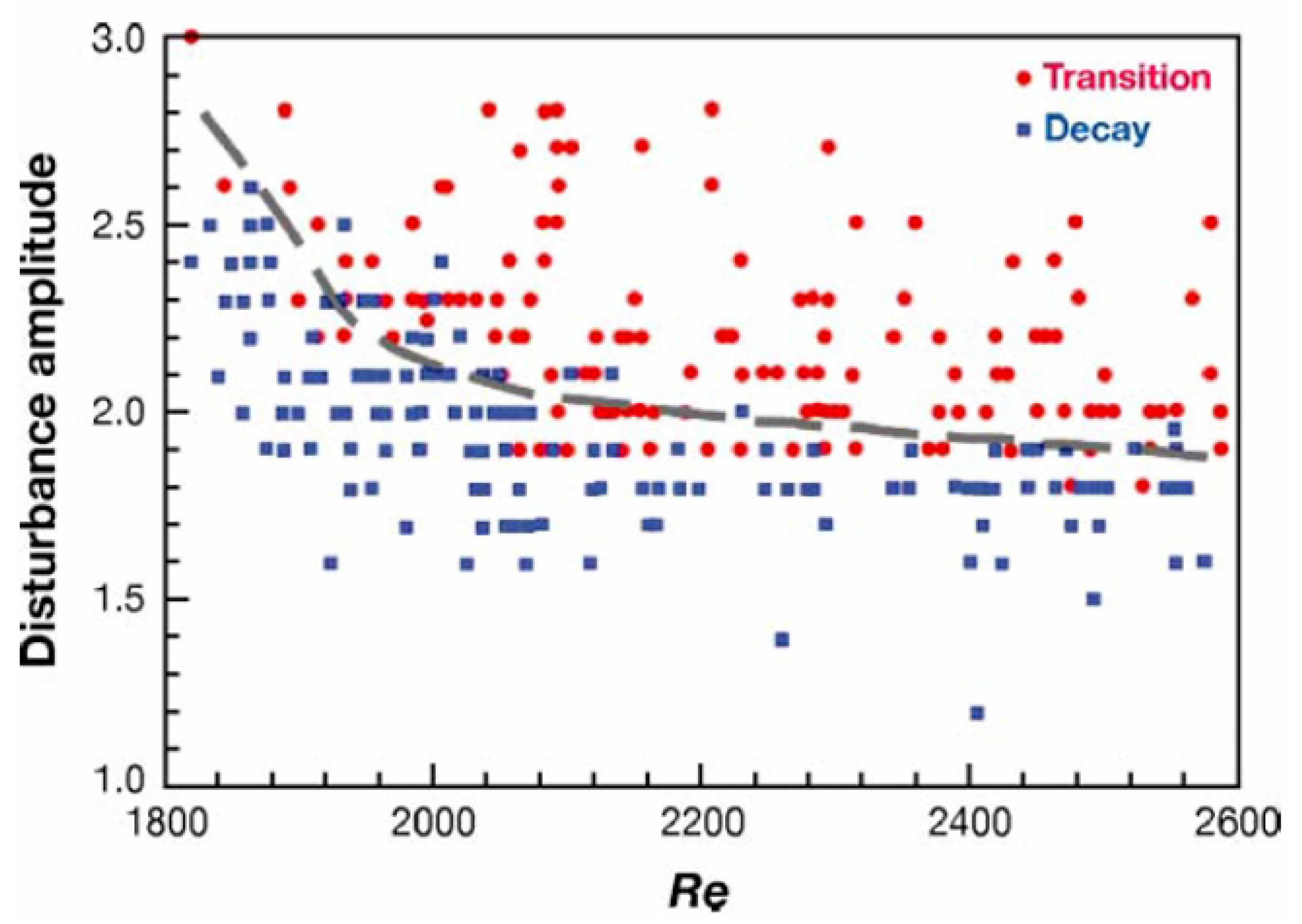
Figure 13: The transition Reynolds number varies with the freestream disturbance level. Circular markers: cases with flow transitioned to turbulence; square markers: cases with disturbances decayed, and the flow remained laminar. Reprinted with permission from Darbyshire and Mullin [83]. Copyright 1995 Cambridge University Press.
Wygnanski et al. [85,86] observed that localized disturbances in pipe flow can generate localized turbulent regions, which can be analogously viewed as coherent structures in circular pipes. These coherent structures typically have a streamwise length of 20 to 30 pipe diameters and maintain relatively constant lengths as they propagate downstream. During transition, turbulence always first occurs locally (not necessarily at the inlet). At relatively low Reynolds numbers (2000–2300), intermittent localized turbulent regions may appear in the pipe. These regions are referred to as puffs and maintain a length of approximately 20 pipe diameters. At higher Reynolds numbers, the intermittently appearing turbulent regions are generally termed slugs. Both puffs and slugs are turbulent regions in circular pipes, but they are distinguished by different Reynolds number ranges. The primary difference is that puffs maintain an almost constant size, whereas slugs grow in both upstream and downstream directions, eventually filling the entire pipe flow.
The development of turbulent spots in pipe flow is strongly dependent on the Reynolds number, and many scholars have investigated this phenomenon [87,88,89]. Similar to flat-plate boundary layer flow, turbulent spots in pipe flow exhibit an arrowhead shape, with a distinct upstream front and a blurred downstream front, separated by a turbulent region. For puff structures, turbulence is not continuously sustained; instead, new turbulence is constantly generated at the upstream front, while turbulent kinetic energy gradually dissipates downstream, eventually reaching an equilibrium state. At Re = 2000, the puff structure maintains an almost constant streamwise length over time, indicating that the upstream and downstream fronts of the puff move at nearly the same velocity, keeping the puff length relatively unchanged. In contrast, at Reynolds numbers of 2600 and 5000, the slug structure clearly exhibits continuous growth in length, eventually filling the entire pipe flow with turbulence.
Hof et al. [90] employed a stereoscopic PIV system to obtain the three-dimensional velocity field in a plane perpendicular to the axis of a circular pipe. They observed various traveling wave states within the Reynolds number range of 2000 to 6000. Their results indicate that these traveling waves in the pipe persist for extended periods. Based on their experimental findings, they proposed that turbulence in the pipe is organized around several dominant traveling waves, which resembles the hypothesis proposed by Lee (2000) that boundary layer turbulence is induced by SCS and their induced vortex structures. Wu et al. [91] simulated a spatially developing pipe flow (Re = 6500) spanning laminar-to-turbulent transition in a 500-radius-long pipe, revealing that mature turbulent spots comprise near-wall reverse hairpin vortices (heads upstream) and core-region forward hairpin vortices. Ruan et al. [92] analyse vortex surface evolution in transitional pipe flows. Their DNS study captured clear vortical structure dynamics during pipe flow transition from laminar to turbulent regimes.
Wu et al. [93] employed direct numerical simulation to investigate the development of puffs and slugs in pipe flow. Using the Lagrangian particle tracking method (including timelines and material surfaces), they studied the early structural evolution of puffs. Their research revealed that turbulence is always generated upstream of puffs and slugs. At a Reynolds number Re = 2200, Fig. 14 shows timeline visualization of 3D waves, low-speed streaks and a typical induced vortex upstream of the puff. It can be observed that these SCSs cause peak-like pattern in the timeline surface. Furthermore, Fig. 15, obtained using the instantaneous vorticity deviation (IVD) method, displays the hairpin vortices surrounding the SCS in Fig. 14. The study by Wu et al. demonstrated that at Re = 2200, SCSs emerge in the early stages upstream of the puff, and these SCSs are associated with regions of high vorticity. When the amplitude of the three-dimensional waves is sufficiently large and persistent, a high-shear layer forms at their edges, promoting vortex development on both sides of the waves. Additionally, the timeline surface results indicate that multiple three-dimensional waves lift up from the near-wall region, forming low-speed streaks. At higher Reynolds numbers (Re = 3000 and 4000), low-speed streaks and SCSs also appear upstream of slugs in pipe flow. However, compared to the case at Re = 2200, the vortices’ generation process induced by SCSs occurs more rapidly, while the underlying physical mechanism remains unchanged. The traveling waves in pipe flow experimentally observed by Hof et al. may be the same as the SCS observed here.
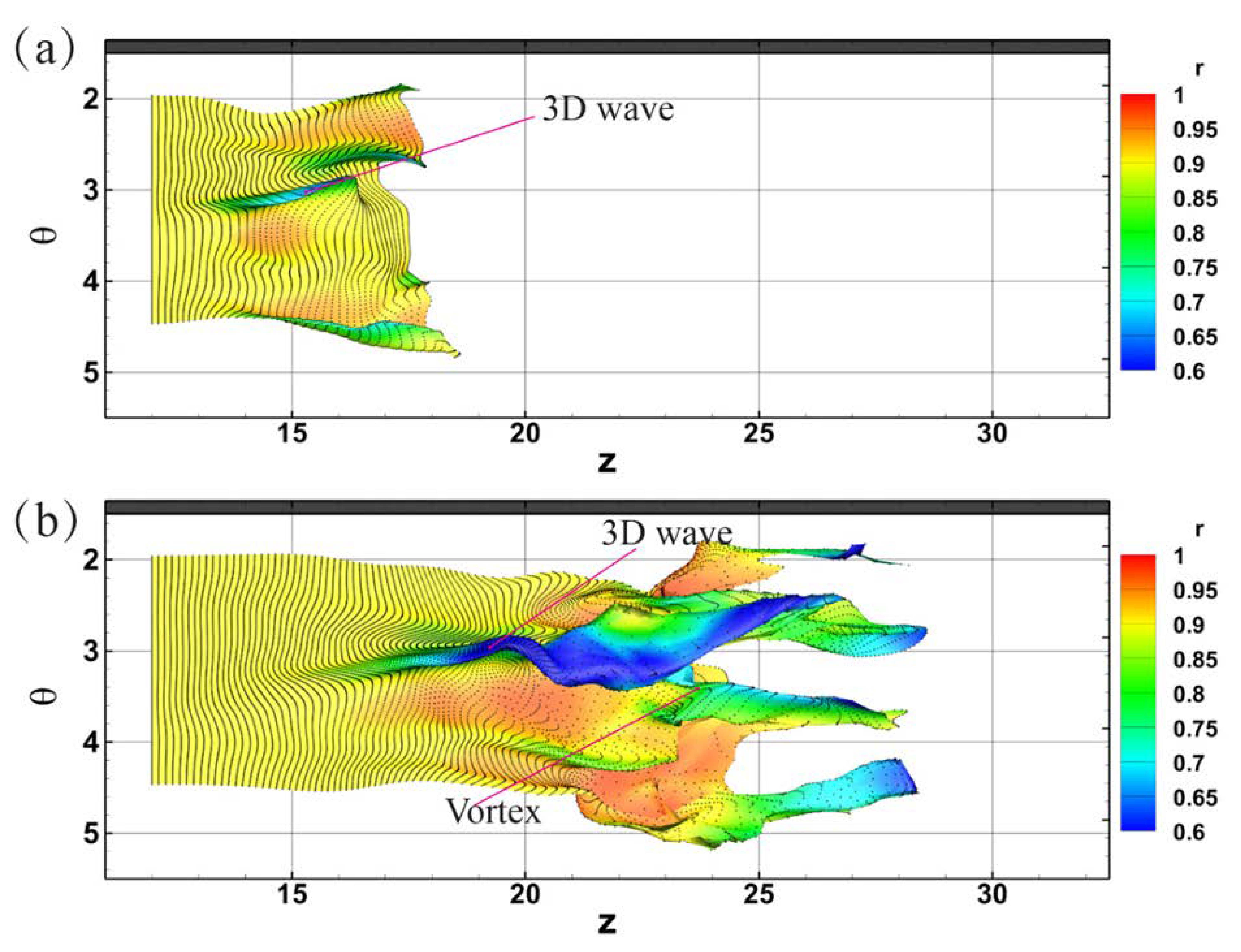
Figure 14: Lagrangian timeline visualization of 3D waves, low-speed streaks and a typical induced vortex in a pipe flow at Re = 2200. Timelines initiated at z = 12, r = 0.9, θ = 2~4.5, and t = 50.0. Tracking time (a) t = 57.0, (b) t = 67.0. Reprinted with permission from Wu et al. [93]. Copyright 2025 AIP Publishing.
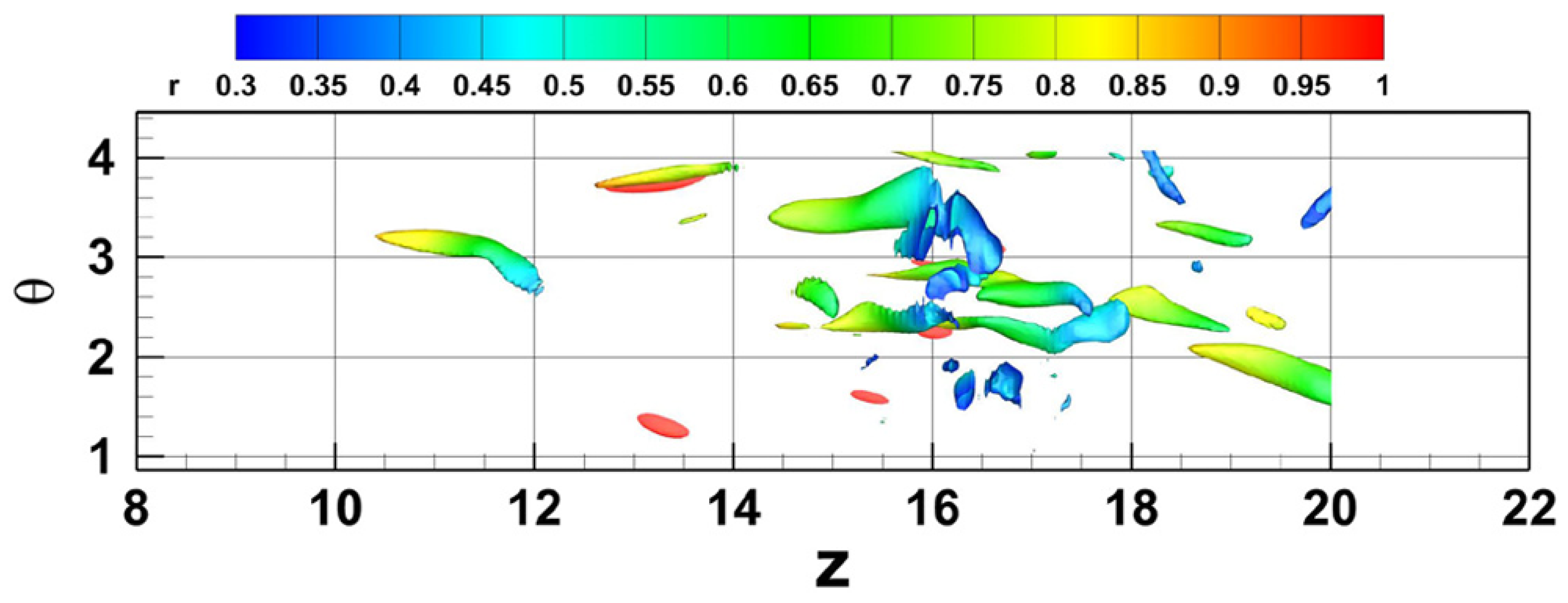
Figure 15: Vortical structures identified using instantaneous vorticity deviation method around a SCS. Reprinted with permission from Wu et al. [93]. Copyright 2025 AIP Publishing.
Regarding the origin of turbulent boundary layers, Theodorsen [94,95] first proposed the theoretical hypothesis that two-dimensional vortex tubes, when disturbed and lifted, would form hairpin vortices. Subsequently, Kline et al. [14] suggested through their seminal experiments that turbulence originates from bursting phenomena, though the underlying mechanism remained unclear for decades. It was not until 2000 that Lee’s research revealed that the dynamical behavior of bursting is governed by SCS structures, thereby connecting these theories. Jiang et al. [47] further elucidated the close relationship between turbulent bursting and SCS structures, showing that near-wall streaks in turbulent boundary layers are fundamentally composed of SCS.
Al-Shamaa et al. [96] experimentally investigated the steady three-dimensional patterns of gravity-driven thin film flows over an inclined sinusoidal bottom profile (Fig. 16). The experiment used silicone oil as the fluid. Within the ranges of Reynolds number (Re = 10–60) and inclination angle (θ = 10°–45°), by combining shadow imaging with light sheet imaging techniques, two unique free surface patterns were revealed: synchronous patterns and checkerboard patterns. The synchronous patterns have a streamwise wavelength that matches the bottom contour of the channel, whereas the checkerboard patterns exhibit surface undulations opposite to the bottom contour. The synchronous pattern exists for all inclination angles, while the checkerboard pattern only appears at high inclination angles (θ > 25°) and higher Reynolds numbers. Both patterns are formed in the regions of peak free surface amplitudes, significantly suppressing the traveling waves and enhancing the flow stability. The transverse wavelength of both patterns decreases as the Reynolds number increases. The three-dimensional flow patterns observed using the light sheet technique exhibit remarkable similarity with the SCSs observed by Jiang et al. through material surfaces. This finding suggests that SCS may also exist in gravity-driven film flows.
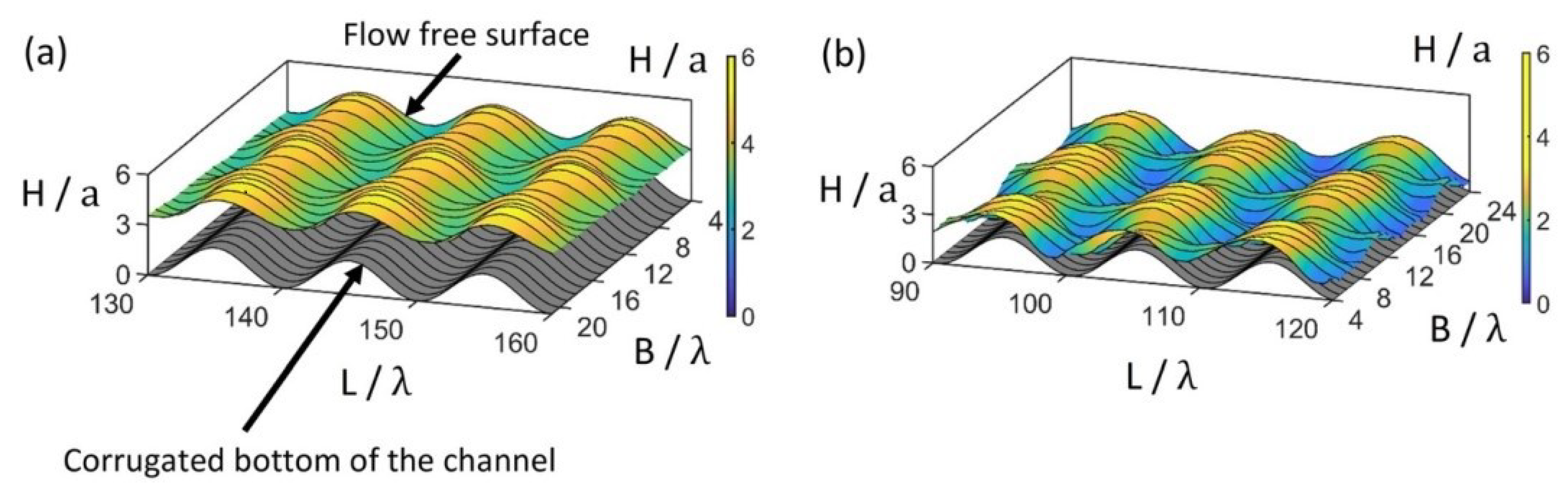
Figure 16: Two types of three-dimensional patterns in a gravity-driven thin film flow: (a) synchronous pattern at Re = 39 and θ = 15°, (b) checkerboard pattern at Re = 39 and θ = 45°. Reprinted with permission from Al-Shamaa et al. [96]. Copyright 2023 AIP Publishing.
Chen et al. [97,98] systematically investigated the transition process in a spatially developing compressible mixing layer using DNS. Their study revealed that the early transition stage is characterized by a coherent coupling between localized 3D waves and developing vortex structures, as evidenced by comprehensive flow visualizations. The evolutionary process, illustrated in Fig. 17, demonstrates the simultaneous development of disturbance waves (represented by positive conditioned normal velocity v) and vortical structures (identified through the Q-criterion) from the inlet to downstream regions. The numerical results by Chen et al. showed that near the inlet, initially two-dimensional vortex tubes undergo rapid three-dimensional deformation due to resonance of the oblique wave mode. This instability triggers a sequence of topological transformations: the wavy spanwise vortices experience vertical displacement before reorganizing into staggered Λ-shaped vortices through convective stretching. These Λ-structures subsequently evolve into hairpin vortices through further deformation, ultimately breaking down into fine-scale turbulent structures. Chen et al.’s analysis further reveals that Λ-vortex formation occurs preferentially in high-shear regions, with statistical results confirming that streamwise vorticity generation coincides with the rapid growth phase of oblique wave modes. Their conditional statistical analysis emphasizes the critical relationship between localized shear intensification and enstrophy production. The researchers suggest that the complete vortex formation mechanism results from a complex interplay between three-dimensional wave propagation and mean shear flow deformation.
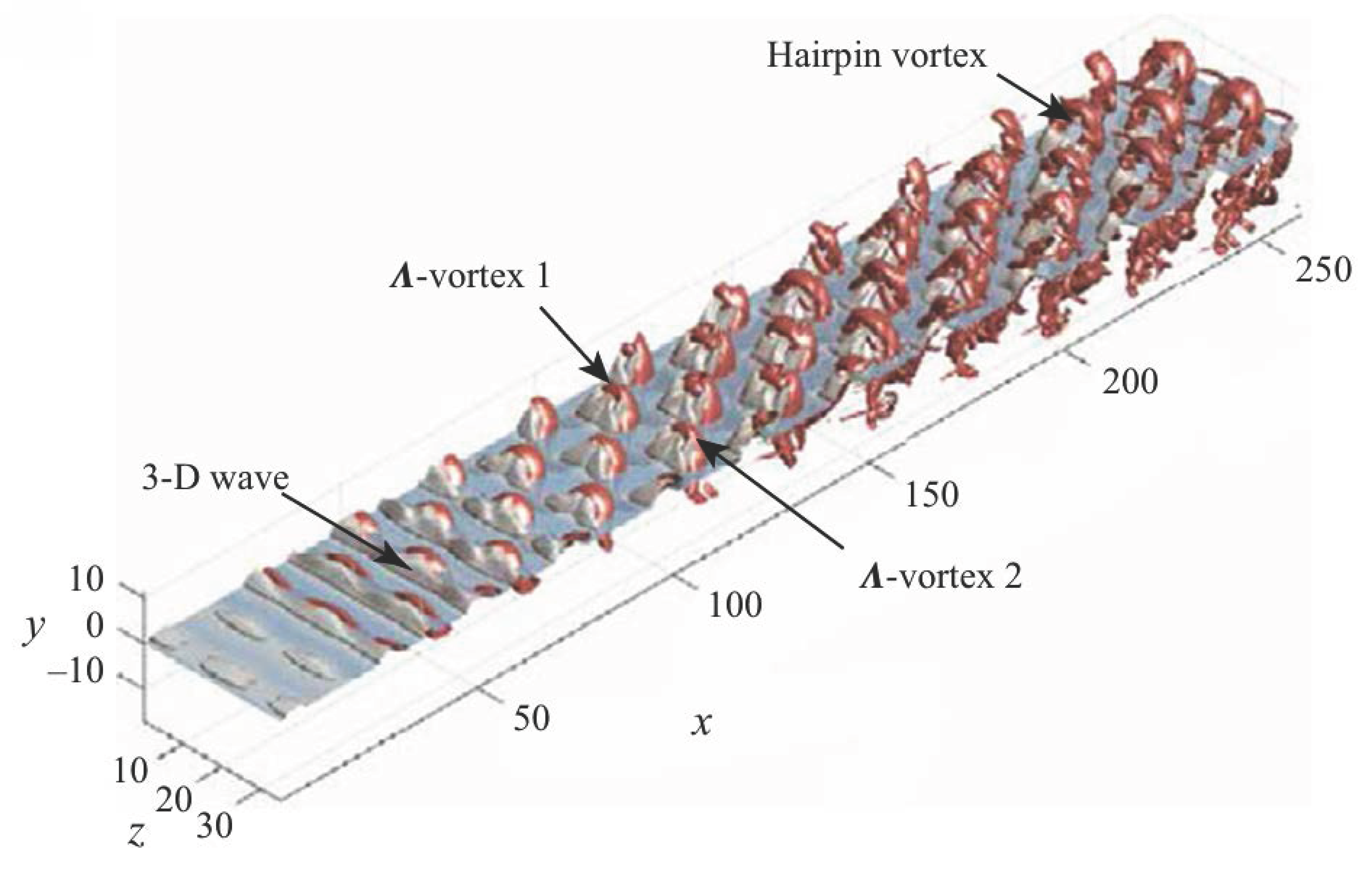
Figure 17: Spatial characteristics of perturbation waves and vortical structures within a mixing layer. The wave structures are visualized by iso-surfaces of the conditioned normal velocity at the plane of yc = 0.08 near the mixing layer centre; the vortex structures are constructed by iso-surfaces of the second invariant of velocity gradient tensor, i.e. Q = 8 × 10⁻³. Reprinted with permission from Chen et al. [97]. Copyright 2025 Cambridge University Press.
Niu et al. [99] investigate turbulence generation in the transitional flow in the wake behind a sphere, as shown in Fig. 18. The study found that as the Reynolds number increased from 250 to 270, the wake transitioned from a dual-vortex structure to a three-dimensional “kink” instability mode, with velocity perturbation amplitudes of approximately 0.25% of the freestream velocity. At Re = 280, regular three-dimensional wave packets formed, propagating at 78% of the freestream velocity. As Re further increased to 300–350, the wave packets sharpened and coupled with hairpin vortices to form stable SCS. Within the Re range of 350–1000, the study revealed three key characteristics: First, the negative velocity perturbation wave packets maintained solitary wave properties in the near-wake region. Second, the negative peak of the streamwise velocity (u) dominated the transition process. Third, the velocity fluctuation patterns transitioned from single-peak/valley to multi-peak/valley configurations. Using the
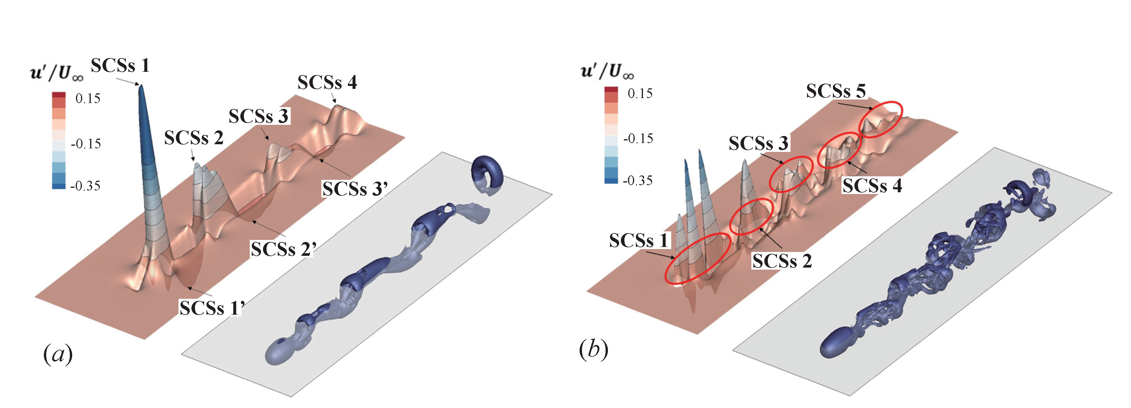
Figure 18: Comparison of the spatial positions of SCSs (extracted from
Jiang et al. [101] systematically studied the evolution mechanism of Holmboe waves into hairpin vortices in stratified shear layers. As shown in Fig. 19, Holmboe waves are generated by the interaction between velocity shear and density gradient, and maintain a regular shape under low turbulence intensity. As the Reynolds number and the inclination angle increase, the turbulence intensifies, the Holmboe waves become unstable, triggering three-dimensional secondary instability. High shear layers form near the wave crest and wave body, generating strong vorticity in the streamline direction, which then develops into hairpin vortices. Hairpin vortices exhibit a head-to-leg structure, with morphological changes in different stages of turbulence development, and also interact with the density interface in various ways to promote mixing. Fig. 19 also shows the schematic diagram of the generation of hairpin vortices from Holmboe waves proposed by Jiang et al. This is similar to mechanism of vortex generation based on SCS proposed by Lee et al. in the boundary layer, indicating that SCSs play a crucial role in the process of vortex generation in stratified shear flows, highlighting the universality of SCS in the vortex generation mechanism.
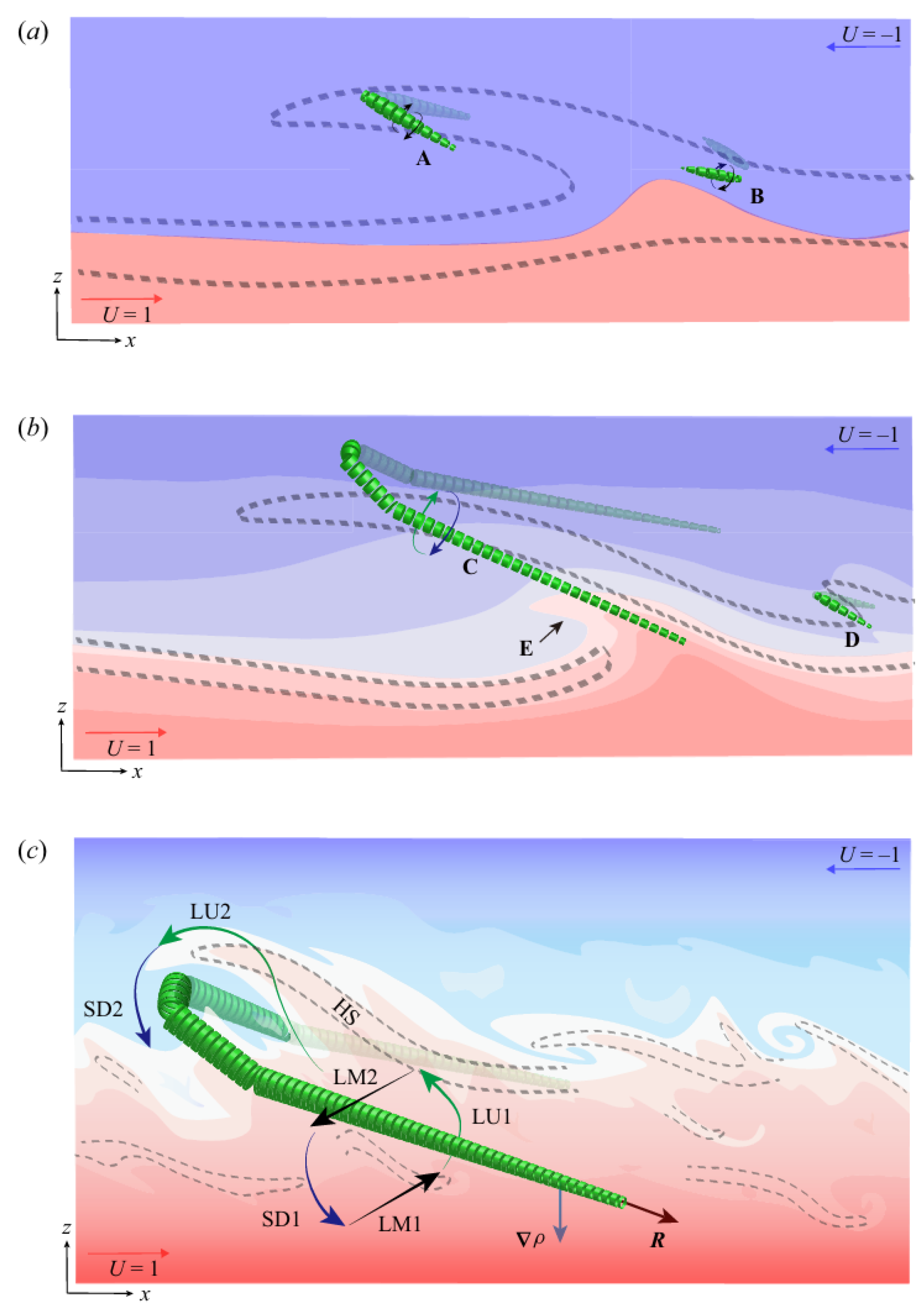
Figure 19: Schemetic view of formation of hairpin vortex in increasingly turbulent stratified shear layers: (a) the origin of a hairpin vortex, (b) its evolution in intermittent regime, (c) its evolution in turbulent regime. Dashed lines indicate shear structure, and the vortices are indicated by green segmented tubes A–D, of which the direction is represented by the rortex vector R. HS: high shear; LU: lift up; SD: sweep down; LM: lateral movement; E: unstable interface. Blue for low density and red for high density. Reprinted with permission from Jiang et al. [101]. Copyright 2022 Cambridge University Press.
Hu et al. [102] employed DNS to investigate wave structures in incompressible circular jets and their role in the generation and evolution of turbulence. Using the Lagrangian material surface tracking method, they found that the formation of SCSs was closely related to high-speed streaks and detailed the dynamic evolution process of these wave packets (see Fig. 20). Further analysis revealed that the propagation speed of the SCS was approximately 60%–90% of the local flow velocity, a pattern consistent with the SCS observed in flat-plate boundary layer flows. The study demonstrated that SCS in circular jets emerge before vortex structures and play a crucial role in flow evolution: As these SCSs develop, they induce the formation of large-scale vortex structures, ultimately driving the flow transition to a turbulent state.
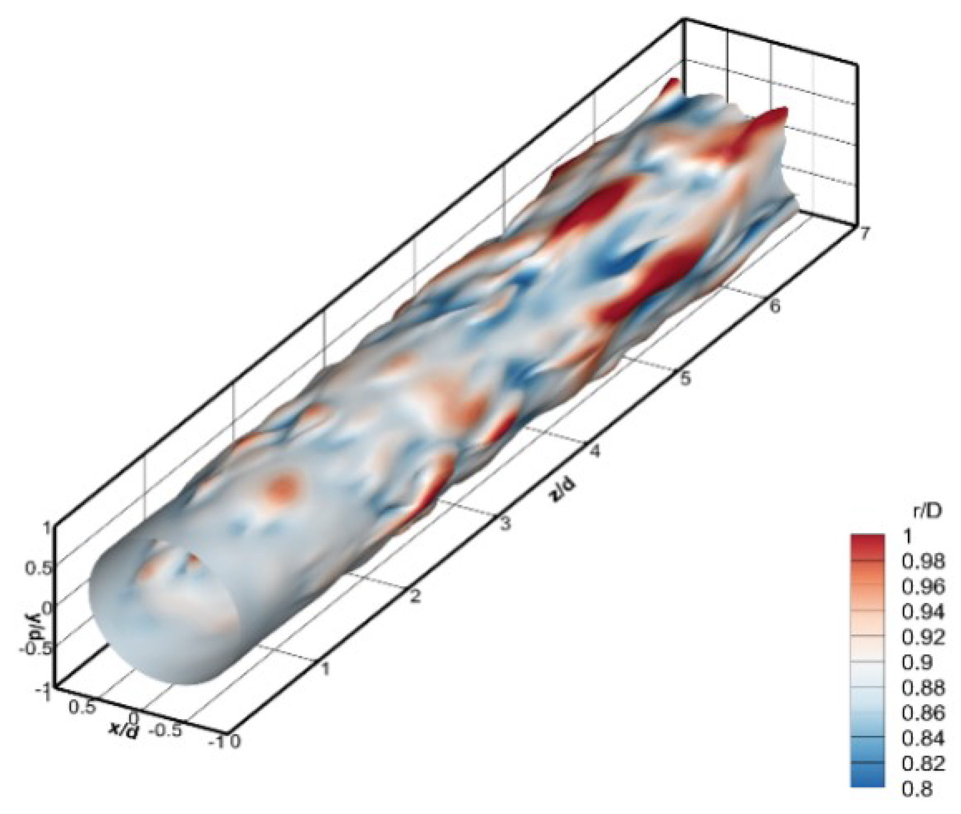
Figure 20: Material surfaces showing the SCSs in round jet flows. Reprinted with permission from Hu et al. [102].
Empirical observations of the SCS across diverse flow regimes mentioned above reveal fundamental commonalities that transcend specific flow configurations. The SCS framework provides a unified interpretive model, extending beyond mere phenomenological similarities. For instance, the mechanism of vortex generation in both boundary-layer and stratified shear-layer flows stems from a shared wave-induced vortex dynamics, a critical SCS-driven process common to these regimes. The conceptual significance of the SCS framework offers promising directions for future research to further test its universality hypothesis.
This article attempts to summarize SCSs discovered in various flows through past experiments and numerical simulations. In previous studies, the role of SCS in turbulence generation has not received sufficient attention. In this Review, we elucidate the properties of SCS and clarify their distinctions from the CS-solitons discovered by Kachanov et al. Subsequently, we systematically categorize the SCS observed in different types of flows. These studies of SCSs have significantly advanced our understanding of turbulence generation and transition mechanisms in wall-bounded flows. During the past three decades, extensive experimental and numerical investigations have demonstrated that SCSs are not merely isolated phenomena, but rather universal features observed across diverse flow configurations, including boundary layers, pipe flows, mixing layers, and stratified shear flows. SCS arises from nonlinear interactions of a pair of oblique waves and exhibits remarkable coherence and longevity compared to other coherent structures.
SCSs play a pivotal role in the formation of key flow features such as low-speed streaks, hairpin vortices, and chain of ring vortices. Their dynamic behavior—marked by lifting up and shear layer formation—serves as a fundamental mechanism for vorticity generation and turbulence production. Notably, the universality of SCSs is evident in their presence across various transition scenarios (K-type, N-type, and O-type) and their analogous manifestations in other flow systems, such as gravity-driven films and jet flows. Nevertheless, further research is needed to explore the causality and dynamics of certain specific structure under varying boundary conditions. The generalization based on the SCS-induced vortex and transition underscores their importance as a unifying framework for explaining turbulence generation in fluid dynamics. Therefore, future research should investigate both active (e.g., localized suction/blowing, plasma actuation) and passive (e.g., riblets, surface textures) flow control strategies aimed at modulating the evolutionary dynamics of SCSs. By suppressing the amplitude growth of SCSs during their development, these control approaches may delay transition and reduce turbulent skin-friction drag in practical applications.
In summary, SCSs represent a cornerstone in the study of wall-bounded turbulence, bridging gaps between disparate theories and providing a cohesive explanation for the transition process. Their continued investigation promises to unlock new insights into the complex nature of fluid turbulence.
Acknowledgement:
Funding Statement: This study was supported by the National Key Project (GJXM92579).
Author Contributions: The authors confirm contribution to the paper as follows: study conception and design: Cunbiao Lee; data collection: Ning Hu, Cunbiao Lee; draft manuscript preparation: Ning Hu, Cunbiao Lee. All authors reviewed the results and approved the final version of the manuscript.
Availability of Data and Materials: The data that support this review are available from the corresponding author, Cunbiao Lee, upon reasonable request, and many figures are reprinted with permission from other researchers.
Ethics Approval: Not applicable.
Conflicts of Interest: The authors declare no conflicts of interest to report regarding the present study.
References
1. Reynolds O . An experimental investigation of the circumstances which determine whether the motion of water shall be direct or sinuous, and of the law of resistance in parallel channels. Phil Trans R Soc Lond. 1883; 174: 935– 82. doi:10.1098/rstl.1883.0029. [Google Scholar] [CrossRef]
2. Morkovin MV . On the many faces of transition. In: Viscous Drag Reduction. Proceedings of the Symposium on Viscous Drag Reduction; 1968 Sep 24–25; Dallas, TX, USA. Boston, MA, USA: Springer; 1969. p. 1– 31. doi:10.1007/978-1-4899-5579-1_1. [Google Scholar] [CrossRef]
3. Wu X , Dong M . A local scattering theory for the effects of isolated roughness on boundary-layer instability and transition: transmission coefficient as an eigenvalue. J Fluid Mech. 2016; 794: 68– 108. doi:10.1017/jfm.2016.125. [Google Scholar] [CrossRef]
4. Zhong X , Wang X . Direct numerical simulation on the receptivity, instability, and transition of hypersonic boundary layers. Annu Rev Fluid Mech. 2012; 44( 1): 527– 61. doi:10.1146/annurev-fluid-120710-101208. [Google Scholar] [CrossRef]
5. Tollmien W . Über die entstehung der turbulenz. In: Vorträge aus dem Gebiete der Aerodynamik und verwandter Gebiete: Aachen 1929. Berlin/Heidelberg, Germany: Springer; 1930. p. 18– 21. doi:10.1007/978-3-662-33791-2_4. [Google Scholar] [CrossRef]
6. Lin CC . On the stability of two-dimensional parallel flows. I. General theory. Quart Appl Math. 1945; 3( 2): 117– 42. doi:10.1090/qam/13983. [Google Scholar] [CrossRef]
7. Landau LD . On the problem of turbulence. Dokl Akad Nauk USSR. 1944; 44: 311. [Google Scholar]
8. Herbert T . Secondary instability of boundary layers. Annu Rev Fluid Mech. 1988; 20: 487– 526. doi:10.1146/annurev.fl.20.010188.002415. [Google Scholar] [CrossRef]
9. Craik ADD . Non-linear resonant instability in boundary layers. J Fluid Mech. 1971; 50( 2): 393– 413. doi:10.1017/S0022112068001965. [Google Scholar] [CrossRef]
10. Schmid PJ . Nonmodal stability theory. Annu Rev Fluid Mech. 2007; 39( 1): 129– 62. doi:10.1146/annurev.fluid.38.050304.092139. [Google Scholar] [CrossRef]
11. Hama FR , Long JD , Hegarty JC . On transition from laminar to turbulent flow. J Appl Phys. 1957; 28( 4): 388– 94. doi:10.1063/1.1722760. [Google Scholar] [CrossRef]
12. Lee CB . New features of CS solitons and the formation of vortices. Phys Lett A. 1998; 247( 6): 397– 402. doi:10.1016/S0375-9601(98)00582-9. [Google Scholar] [CrossRef]
13. Wu X , Moin P , Wallace JM , Skarda J , Lozano-Durán A , Hickey JP . Transitional-turbulent spots and turbulent-turbulent spots in boundary layers. Proc Natl Acad Sci U S A. 2017; 114( 27): E5292– 99. doi:10.1073/pnas.1704671114. [Google Scholar] [CrossRef]
14. Kline SJ , Reynolds WC , Schraub FA , Runstadler PW . The structure of turbulent boundary layers. J Fluid Mech. 1967; 30( 4): 741– 73. doi:10.1017/S0022112067001740. [Google Scholar] [CrossRef]
15. Kim HT , Kline SJ , Reynolds WC . The production of turbulence near a smooth wall in a turbulent boundary layer. J Fluid Mech. 1971; 50( 1): 133– 60. doi:10.1017/S0022112071002490. [Google Scholar] [CrossRef]
16. Offen GR , Kline SJ . A proposed model of the bursting process in turbulent boundary layers. J Fluid Mech. 1975; 70( 2): 209– 28. doi:10.1017/S002211207500198X. [Google Scholar] [CrossRef]
17. Schoppa W , Hussain F . Coherent structure generation in near-wall turbulence. J Fluid Mech. 2002; 453: 57– 108. doi:10.1017/S002211200100667X. [Google Scholar] [CrossRef]
18. Singer BA , Joslin RD . Metamorphosis of a hairpin vortex into a young turbulent spot. Phys Fluids. 1994; 6( 11): 3724– 36. doi:10.1063/1.868363. [Google Scholar] [CrossRef]
19. Lee CB . Possible universal transitional scenario in a flat plate boundary layer: measurement and visualization. Phys Rev E. 2000; 62( 3): 3659. doi:10.1103/PhysRevE.62.3659. [Google Scholar] [CrossRef]
20. Lee CB , Hong ZX , Kachanov YS , Borodulin VI , Gaponenko VV . A study in transitional flat plate boundary layers: measurement and visualization. Exp Fluids. 2000; 28: 243– 51. doi:10.1007/s003480050384. [Google Scholar] [CrossRef]
21. Kachanov YS . Physical mechanisms of laminar-boundary-layer transition. Annu Rev Fluid Mech. 1994; 26( 1): 411– 82. doi:10.1146/annurev.fl.26.010194.002211. [Google Scholar] [CrossRef]
22. Meyer DGW , Rist U , Borodulin VI , Gaponenko VR , Kachanov YS , Lian QX . Late-stage transitional boundary-layer structures. Direct numerical simulation and experiment. In: Fasel HF , Saric WS , editors. Laminar-Turbulent Transition. IUTAM Symposia. Berlin/Heidelberg, Germany: Springer; 2000. p. 167– 72. doi:10.1007/978-3-662-03997-7_23. [Google Scholar] [CrossRef]
23. Perry AE , Lim TT , Teh EW . A visual study of turbulent spots. J Fluid Mech. 1981; 104: 387– 405. doi:10.1017/S0022112081002966. [Google Scholar] [CrossRef]
24. Gad-El-Hak M , Blackwelderf RF , Riley JJ . On the growth of turbulent regions in laminar boundary layers. J Fluid Mech. 1981; 110: 73– 95. doi:10.1017/S002211208100061X. [Google Scholar] [CrossRef]
25. Michael D , Daniel F . Exact coherent states and the nonlinear dynamics of wall-bounded turbulent flows. Annu Rev Fluid Mech. 2021; 53( 1): 227– 53. doi:10.1146/annurev-fluid-051820-020223. [Google Scholar] [CrossRef]
26. Wang YX , Choi KS , Gaster M , Atkin C , Borodulin V , Kachanov Y . Early development of artificially initiated turbulent spots. J Fluid Mech. 2021; 916: A1. doi:10.1017/jfm.2021.152. [Google Scholar] [CrossRef]
27. Wu X . New insights into turbulent spots. Annu Rev Fluid Mech. 2023; 55( 1): 45– 75. doi:10.1146/annurev-fluid-120720-021813. [Google Scholar] [CrossRef]
28. Lee CB , Wu JZ . Transition in wall-bounded flows. Appl Mech Rev. 2008; 61( 3): 030802. doi:10.1115/1.2909605. [Google Scholar] [CrossRef]
29. Lee C , Jiang X . Flow structures in transitional and turbulent boundary layers. Phys Fluids. 2019; 31( 11): 111301. doi:10.1063/1.5121810. [Google Scholar] [CrossRef]
30. Smith CR , Paxson RD . A technique for evaluation of three-dimensional behavior in turbulent boundary layers using computer augmented hydrogen bubble-wire flow visualization. Exp Fluids. 1983; 1( 1): 43– 9. doi:10.1007/BF00282266. [Google Scholar] [CrossRef]
31. Acarlar MS , Smith CR . A study of hairpin vortices in a laminar boundary layer. Part 1. Hairpin vortices generated by a hemisphere protuberance. J Fluid Mech. 1987; 175: 1– 41. doi:10.1017/S0022112087000272. [Google Scholar] [CrossRef]
32. Lu LJ , Smith CR . Image processing of hydrogen bubble flow visualization for determination of turbulence statistics and bursting characteristics. Exp Fluids. 1985; 3( 6): 349– 56. doi:10.1007/BF01830195. [Google Scholar] [CrossRef]
33. Lu LJ . Image processing of hydrogen bubble flow visualization for quantitative evaluation of hairpin-type vortices as a flow structure of turbulent boundary layers [ master’s thesis]. Bethlehem, PA, USA: Lehigh University; 1988. [Google Scholar]
34. Acarlar MS , Smith CR . A study of hairpin vortices in a laminar boundary layer. Part 2. Hairpin vortices generated by fluid injection. J Fluid Mech. 1987; 175: 43– 83. doi:10.1017/S0022112087000284. [Google Scholar] [CrossRef]
35. Haidari AH , Smith CR . The generation and regeneration of single hairpin vortices. J Fluid Mech. 1994; 277: 135– 62. doi:10.1017/S0022112094002715. [Google Scholar] [CrossRef]
36. Crane RJ , Popinhak AR , Martinuzzi RJ , Morton C . Tomographic PIV investigation of vortex shedding topology for a cantilevered circular cylinder. J Fluid Mech. 2022; 931: R1. doi:10.1017/jfm.2021.904. [Google Scholar] [CrossRef]
37. Feng Z , Ye Q . Turbulent boundary layer over porous media with wall-normal permeability. Phys Fluids. 2023; 35( 9): 095111. doi:10.1063/5.0160773. [Google Scholar] [CrossRef]
38. Tu H , Wang Z , Gao Q , She W , Wang F , Wang J , et al. Tomographic PIV investigation on near-wake structures of a hemisphere immersed in a laminar boundary layer. J Fluid Mech. 2023; 971: A36. doi:10.1017/jfm.2023.621. [Google Scholar] [CrossRef]
39. Schröder A , Schanz D , Bosbach J , Novara M , Geisler R , Agocs J , et al. Large-scale volumetric flow studies on transport of aerosol particles using a breathing human model with and without face protections. Phys Fluids. 2022; 34: 035133. doi:10.1063/5.0086383. [Google Scholar] [CrossRef]
40. Schröder A , Schanz D . 3D Lagrangian particle tracking in fluid mechanics. Annu Rev Fluid Mech. 2023; 55( 1): 511– 40. doi:10.1146/annurev-fluid-031822-041721. [Google Scholar] [CrossRef]
41. Elsinga G , Kuik DJ , Van Oudheusden B , Scarano F . Investigation of the three-dimensional coherent structures in a turbulent boundary layer with tomographic-PIV. In: Proceedings of the 45th AIAA Aerospace Sciences Meeting and Exhibit; 2007 Jan 8–11; Reno, Nevada. doi:10.2514/6.2007-1305. [Google Scholar] [CrossRef]
42. Lin J , Laval JP , Foucaut JM , Stanislas M . Quantitative characterization of coherent structures in the buffer layer of near-wall turbulence. Part 1: Streaks. Exp Fluids. 2008; 45( 6): 999– 1013. doi:10.1007/s00348-008-0522-4. [Google Scholar] [CrossRef]
43. Dennis DJC , Nickels TB . Experimental measurement of large-scale three-dimensional structures in a turbulent boundary layer. Part 1. Vortex packets. J Fluid Mech. 2011; 673: 180– 217. doi:10.1017/S0022112010006324. [Google Scholar] [CrossRef]
44. Tang ZQ , Jiang N , Schröder A , Geisler R . Tomographic PIV investigation of coherent structures in a turbulent boundary layer flow. Acta Mech Sin. 2012; 28( 3): 572– 82. doi:10.1007/s10409-012-0082-y. [Google Scholar] [CrossRef]
45. Gao Q , Ortiz-Dueñas C , Longmire EK . Evolution of coherent structures in turbulent boundary layers based on moving tomographic PIV. Exp Fluids. 2013; 54: 1– 16. doi:10.1007/s00348-013-1625-0. [Google Scholar] [CrossRef]
46. Schröder A , Geisler R , Elsinga GE , Scarano F , Dierksheide U . Investigation of a turbulent spot and a tripped turbulent boundary layer flow using time-resolved tomographic PIV. Exp Fluids. 2008; 44: 305– 16. doi:10.1007/s00348-007-0403-2. [Google Scholar] [CrossRef]
47. Jiang XY , Lee CB , Smith CR , Chen JW , Linden PF . Experimental study on low-speed streaks in a turbulent boundary layer at low Reynolds number. J Fluid Mech. 2020; 903: A6. doi:10.1017/jfm.2020.617. [Google Scholar] [CrossRef]
48. Jiang XY , Lee CB , Chen X , Smith CR , Linden PF . Structure evolution at early stage of boundary-layer transition: simulation and experiment. J Fluid Mech. 2020; 890: A11. doi:10.1017/jfm.2020.107. [Google Scholar] [CrossRef]
49. Jiang XY , Gu DW , Lee CB , Smith CR , Linden PF . A metamorphosis of three-dimensional wave structure in transitional and turbulent boundary layers. J Fluid Mech. 2021; 914: A4. doi:10.1017/jfm.2020.1023. [Google Scholar] [CrossRef]
50. Yang CR , Feng ZH , Lee CB . Self-organized oblique waves upstream of the leading edge of a flat plate. Phys Fluids. 2025; 37( 2): 021714. doi:10.1063/5.0258057. [Google Scholar] [CrossRef]
51. Lee CB , Li R . On the dynamics in a transitional boundary layer. Commun Nonlinear Sci Numer Simul. 2001; 6( 3): 111– 71. doi:10.1016/S1007-5704(01)90000-0. [Google Scholar] [CrossRef]
52. Lee CB , Chen SY . Dynamics of transitional boundary layers. Transit Turbul Control. 2006; 2: 39– 85. doi:10.1142/9789812700896_0002. [Google Scholar] [CrossRef]
53. Lee C , Li R . Dominant structure for turbulent production in a transitional boundary layer. J Turb. 2007; 8: N55. doi:10.1080/14685240600925163. [Google Scholar] [CrossRef]
54. Borodulin VI , Kachanov YS . Role of the mechanism of local secondary instability in K-breakdown of boundary layer. Izv Sib Otd Akad Nauk SSSR Ser Tekh Nauk. 1988; 18: 65– 77. [Google Scholar]
55. Bake S , Fernholz HH , Kachanov YS . Resemblance of K-and N-regimes of boundary-layer transition at late stages. Eur J Mech B/Fluids. 2000; 19( 1): 1– 22. doi:10.1016/S0997-7546(00)00108-4. [Google Scholar] [CrossRef]
56. Bake S , Meyer DGW , Rist U . Turbulence mechanism in Klebanoff transition: a quantitative comparison of experiment and direct numerical simulation. J Fluid Mech. 2002; 459: 217– 43. doi:10.1017/S0022112002007954. [Google Scholar] [CrossRef]
57. Borodulin VI , Gaponenko VR , Kachanov YS , Meyer DGW , Rist U , Lian QX , et al. Late-stage transitional boundary-layer structures. Direct numerical simulation and experiment. Theor Comput Fluid Dyn. 2002; 15: 317– 37. doi:10.1007/s001620100054. [Google Scholar] [CrossRef]
58. Klebanoff PS , Tidstrom KD , Sargent LM . The three-dimensional nature of boundary-layer instability. J Fluid Mech. 1962; 12( 1): 1– 34. doi:10.1017/S0022112062000014. [Google Scholar] [CrossRef]
59. Goldstein ME , Choi SW . Nonlinear evolution of interacting oblique waves on two-dimensional shear layers. J Fluid Mech. 1989; 207: 97– 120. doi:10.1017/S002211208900251X. [Google Scholar] [CrossRef]
60. Berlin S , Lundbladh A , Henningson D . Spatial simulations of oblique transition in a boundary layer. Phys Fluids. 1994; 6( 6): 1949– 51. doi:10.1063/1.868200. [Google Scholar] [CrossRef]
61. Berlin S , Wiegel M , Henningson DS . Numerical and experimental investigations of oblique boundary layer transition. J Fluid Mech. 1999; 393: 23– 57. doi:10.1017/S002211209900511X. [Google Scholar] [CrossRef]
62. Kachanov YS . On a universal mechanism of turbulence production in wall shear flows. Recent Results in Laminar-Turbulent Transition: Selected numerical and experimental contributions from the DFG priority programme ‘Transition’ in Germany. Berlin/Heidelberg, Germany: Springer; 2003. p. 1– 12. doi:10.1007/978-3-540-45060-3_1. [Google Scholar] [CrossRef]
63. Chen WJ . Numerical simulations of boundary layer transition by combined compact difference methods [ dissertation]. Singapore: Nanyang Technological University; 2013. [Google Scholar]
64. Hu N , Du B , Lee C . Internal structures of turbulent spots. Phys Fluids. 2025; 37( 2): 024125. doi:10.1063/5.0254741. [Google Scholar] [CrossRef]
65. Hu N , Zhu YD , Lee CB , Smith CR . Experimental and numerical investigation of turbulent spots in a flat plate boundary layer. J Fluid Mech. 2025; 1008: A37. doi:10.1017/jfm.2025.202. [Google Scholar] [CrossRef]
66. Runstadler PW , Kline SJ , Reynolds WC . An experimental investigation of the flow structure of the turbulent boundary layer [ master’s thesis]. Stanford, CA, USA: Stanford University; 1963. [Google Scholar]
67. Wang W , Pan C , Wang J . Wall-normal variation of spanwise streak spacing in turbulent boundary layer with low-to-moderate Reynolds number. Entropy. 2018; 21( 1): 24. doi:10.3390/e21010024. [Google Scholar] [CrossRef]
68. Smith CR , Metzler SP . The characteristics of low-speed streaks in the near-wall region of a turbulent boundary layer. J Fluid Mech. 1983; 129: 27– 54. doi:10.1017/S0022112083000634. [Google Scholar] [CrossRef]
69. Adeel Z , Yang D , Chen G . Extract and characterize hairpin vortices in turbulent flows. IEEE Trans Vis Comput Graph. 2023; 30( 1): 716– 26. doi:10.1109/TVCG.2023.3326603. [Google Scholar] [CrossRef]
70. Landahl MT . A note on an algebraic instability of inviscid parallel shear flows. J Fluid Mech. 1980; 98( 2): 243– 51. doi:10.1017/S0022112080000122. [Google Scholar] [CrossRef]
71. Landahl MT . On sublayer streaks. J Fluid Mech. 1990; 212: 593– 614. doi:10.1017/S0022112090002105. [Google Scholar] [CrossRef]
72. Kim J , Lim J . A linear process in wall-bounded turbulent shear flows. Phys Fluids. 2000; 12( 8): 1885– 8. doi:10.1063/1.870437. [Google Scholar] [CrossRef]
73. Chernyshenko SI , Baig MF . The mechanism of streak formation in near-wall turbulence. J Fluid Mech. 2005; 544: 99– 131. doi:10.1017/S0022112005006506. [Google Scholar] [CrossRef]
74. Elofsson P . Experiments on oblique transition in wall bounded shear flows [ dissertation]. Stockholm, Sweden: KTH Royal Institute of Technology; 1998. [Google Scholar]
75. Rao KN , Narasimha R , Narayanan MAB . The ’bursting’ phenomenon in a turbulent boundary layer. J Fluid Mech. 1971; 48( 2): 339– 52. doi:10.1017/S0022112071001605. [Google Scholar] [CrossRef]
76. Blackwelder RF , Kaplan RE . On the wall structure of the turbulent boundary layer. J Fluid Mech. 1976; 76( 1): 89– 112. doi:10.1017/S0022112076003145. [Google Scholar] [CrossRef]
77. Jiménez J . The streaks of wall-bounded turbulence need not be long. J Fluid Mech. 2022; 945: R3. doi:10.1017/jfm.2022.572. [Google Scholar] [CrossRef]
78. Morkovin MV , Reshotko E , Herbert T . Transition in open flow systems: a reassessment. Bull Am Phys Soc. 1994; 39( 9): 1– 31. [Google Scholar]
79. Hof B , Juel A , Mullin T . Scaling of the turbulence transition threshold in a pipe. Phys Rev Lett. 2003; 91( 24): 244502. doi:10.1103/PhysRevLett.91.244502. [Google Scholar] [CrossRef]
80. Eckhardt B , Schneider TM , Hof B , Westerweel J . Turbulence transition in pipe flow. Annu Rev Fluid Mech. 2007; 39( 1): 447– 68. doi:10.1146/annurev.fluid.39.050905.110308. [Google Scholar] [CrossRef]
81. Avila M , Barkley D , Hof B . Transition to turbulence in pipe flow. Ann Rev Fluid Mech. 2023; 55( 1): 575– 602. doi:10.1146/annurev-fluid-120720-025957. [Google Scholar] [CrossRef]
82. Pfenninger W . Transition in the inlet length of tubes at high Reynolds numbers. Bound Layer Flow Control. 1961: 970– 80. [Google Scholar]
83. Darbyshire AG , Mullin T . Transition to turbulence in constant-mass-flux pipe flow. J Fluid Mech. 1995; 289: 83– 114. doi:10.1017/S0022112095001248. [Google Scholar] [CrossRef]
84. Salwen H , Cotton FW , Grosch CE . Linear stability of Poiseuille flow in a circular pipe. J Fluid Mech. 1980; 98( 2): 273– 84. doi:10.1017/S0022112080000146. [Google Scholar] [CrossRef]
85. Wygnanski IJ , Champagne FH . On transition in a pipe. Part 1. The origin of puffs and slugs and the flow in a turbulent slug. J Fluid Mech. 1973; 59( 2): 281– 335. doi:10.1017/S0022112073001576. [Google Scholar] [CrossRef]
86. Wygnanski I , Sokolov M , Friedman D . On transition in a pipe. Part 2. The equilibrium puff. J Fluid Mech. 1975; 69( 2): 283– 304. doi:10.1017/S0022112075001449. [Google Scholar] [CrossRef]
87. Song B , Barkley D , Hof B , Avila M . Speed and structure of turbulent fronts in pipe flow. J Fluid Mech. 2017; 813: 1045– 59. doi:10.1017/jfm.2017.14. [Google Scholar] [CrossRef]
88. Lindgren ER . Propagation velocity of turbulent slugs and streaks in transition pipe flow. Phys Fluids. 1969; 12( 2): 418– 25. doi:10.1063/1.1692497. [Google Scholar] [CrossRef]
89. Barkley D , Song B , Mukund V , Lemoult G , Avila M , Hof B . The rise of fully turbulent flow. Nature. 2015; 526( 7574): 550– 3. doi:10.1038/nature15701. [Google Scholar] [CrossRef]
90. Hof B , van Doorne CHW , Westerweel J , Nieuwstadt FTM , Faisst H , Eckhardt B , et al. First experimental observation of coherent traveling wave states in pipe flow. APS Div Fluid Dyn Meet Abstr. 2004; 57: NM- 003. doi:10.1126/science.1100393. [Google Scholar] [CrossRef]
91. Wu X , Moin P , Adrian RJ . Laminar to fully turbulent flow in a pipe: Scalar patches, structural duality of turbulent spots and transitional overshoot. J Fluid Mech. 2020; 896: A9. doi:10.1017/jfm.2020.304. [Google Scholar] [CrossRef]
92. Ruan S , Xiong S , You J , Yang Y . Generation of streamwise helical vortex loops via successive reconnections in early pipe transition. Phys Fluids. 2022; 34: 054112. doi:10.1063/5.0094326. [Google Scholar] [CrossRef]
93. Wu P , Gu D , Jiang X , Lee C . Three-dimensional wave structure within the puff of pipe flow. Phys Fluids. 2025; 37( 2): 024125. doi:10.1063/5.0255936. [Google Scholar] [CrossRef]
94. Theodorsen T . Mechanism of turbulence. In: Proceedings of the 2nd Midwestern Conference on Fluid Mechanics; 1952 March 17–19; Columbus, Ohio, USA. [Google Scholar]
95. Theodorsen T . The structure of turbulence. In: Görtler H , Tollmien W , editors. 50 Jahre Grenzschichtforschung. Wiesbaden, Germany: Vieweg+Teubner Verlag; 1955. p. 55– 62. doi:10.1007/978-3-663-20219-6_6. [Google Scholar] [CrossRef]
96. Al-Shamaa B , Kahraman T , Wierschem A . Steady three-dimensional patterns in gravity-driven film flow down an inclined sinusoidal bottom contour. Phys Fluids. 2023; 35( 3): 033307. doi:10.1063/5.0140841. [Google Scholar] [CrossRef]
97. Chen J , Xiao Z . Existence and characteristics of soliton-like coherent structures in a transitional mixing layer. Phys Fluids. 2025; 37( 7): 071704. doi:10.1063/5.0277845. [Google Scholar] [CrossRef]
98. Chen J , Jiang X , Xiao Z . Wave and vortex structures in transitional mixing layer: a numerical investigation. J Fluid Mech. 2025; 1020: A48. doi:10.1017/jfm.2025.10548. [Google Scholar] [CrossRef]
99. Niu L , Dou HS , Zhou C , Xu W . Solitary wave structure of transitional flow in the wake of a sphere. Phys Fluids. 2025; 37( 1): 014111. doi:10.1063/5.0251193. [Google Scholar] [CrossRef]
100. Niu L , Dou HS , Zhou C , Xu W . Turbulence generation in the transitional wake flow behind a sphere. Phys Fluids. 2024; 36( 3): 034127. doi:10.1063/5.0199349. [Google Scholar] [CrossRef]
101. Jiang X , Lefauve A , Dalziel SB , Linden PF . The evolution of coherent vortical structures in increasingly turbulent stratified shear layers. J Fluid Mech. 2022; 947: A30. doi:10.1017/jfm.2022.588. [Google Scholar] [CrossRef]
102. Hu Z , Yang Y , Cai Q . Detection and Analysis of Soliton-like Coherent Structure in Free Round Jet Flow. Phys Fluids. 2025; 37( 8): 085174. doi:10.1063/5.0280336. [Google Scholar] [CrossRef]
Cite This Article
 Copyright © 2025 The Author(s). Published by Tech Science Press.
This work is licensed under a Creative Commons Attribution 4.0 International License , which permits unrestricted use, distribution, and reproduction in any medium, provided the original work is properly cited.
 Downloads
 Citation Tools