
 Submit a Paper
 Propose a Special lssue
 Open Access
ARTICLE

Optimized Pilot Hydraulic Valves for Urban Water Systems via Enhanced BP-Coati Algorithms
1 School of Petrochemical Technology, Lanzhou University of Technology, Lanzhou, 730050, China
2 Machinery Industry Pump and Special Valve Engineering Research Center, Lanzhou University of Technology, Lanzhou, 730050, China
* Corresponding Author: Xinhao Liu. Email:
Fluid Dynamics & Materials Processing 2025, 21(10), 2495-2526. https://doi.org/10.32604/fdmp.2025.068674
Received 03 June 2025; Accepted 29 August 2025; Issue published 30 October 2025
 View Full Text
 Download PDF
Abstract
Hydraulic control valves, positioned at the terminus of pipe networks, are critical for regulating flow and pressure, thereby ensuring the operational safety and efficiency of pipeline systems. However, conventional valve designs often struggle to maintain effective regulation across a wide range of system pressures. To address this limitation, this study introduces a novel Pilot hydraulic valves specifically engineered for enhanced dynamic performance and precise regulation under variable pressure conditions. Building upon prior experimental findings, the proposed design integrates a high-fidelity simulation framework and a surrogate model-based optimization strategy. The study begins by formulating a comprehensive mathematical model of the pipeline system using electro-hydraulic simulation techniques, capturing the dynamic behavior of both the pilot valve and the broader urban water distribution network. A coupled simulation platform is then developed, leveraging both one-dimensional (1D) and three-dimensional (3D) software tools to accurately analyze the valve’s transient response and operational characteristics. To achieve optimal valve performance, a multi-objective optimization approach is proposed. This approach employs a Levy-based Improved Tuna-Inspired Wake-Up Optimization Algorithm (L-TIWOA) to refine a Backpropagation (BP) neural network, thereby constructing a highly accurate surrogate model. Compared to the conventional BP neural network, the improved model demonstrates significantly reduced mean absolute error (MAE) and mean squared error (MSE), underscoring its superior predictive capability. The surrogate model serves as the objective function within an Improved Multi-Objective Mother Lode Optimization Algorithm (IMOMLOA), which is then used to fine-tune the key design parameters of the control valve. Validation through experimental testing reveals that the optimized valve achieves a maximum flow deviation of just 1.11 t/h, corresponding to a control accuracy of 3.7%, at a target flow rate of 30 t/h. Moreover, substantial improvements in dynamic response are observed, confirming the effectiveness of the proposed design and optimization strategy.Keywords
As a core component of modern urban infrastructure, urban water supply networks face major challenges in safe and efficient operation. As a key regulatory device for pipeline systems, the dynamic characteristics of hydraulic control valves are significantly affected by complex physical phenomena such as non-constant flow, pressure transients and fluid-structure interaction (FSI). These factors are directly related to the stability and reliability of the water supply system. As the “intelligent switch” of the pipeline system, the dynamic characteristics and adjustment accuracy of the hydraulic control valve directly determine the stability and energy efficiency of the entire system.
In terms of research methods, scholars have made important progress: Shadloo et al. [1] developed the Smoothed Particle Hydrodynamics (SPH) method, providing a novel approach for simulating complex flow dynamics during valve actuation. Alberto et al. [2] successfully captured transient flow characteristics induced by pressure fluctuations using dynamic mesh technology. Kalita et al. [3] and Kim et al. [4] explore the application and challenges of the Finite Element Method and Immersed Boundary Method, respectively, in Fluid-Structure Interaction (FSI) problems. Studies by Straus et al. [5], Lee et al. [6], and Diaz-Ibarra et al. [7] have demonstrated the advantages of surrogate models in multi-objective optimization, and multi-objective optimization methods based on surrogate models have broad applications in engineering practice. These method innovations provide powerful tools for valve dynamics performance research.
In terms of mechanism research, Stosiak et al. [8,9] revealed the coupling mechanism between pressure pulsation and valve spool vibration, highlighting the resonance phenomenon that occurs when the spool’s natural frequency matches external excitation—a critical insight for addressing hydraulic control valve vibrations. Aissa-Berraies [10] discovered the flow-induced vibration phenomenon during proportional control. Zhao et al. [11] and Xie et al. [12] studied the influence of structural parameters on the dynamic response of the valve. Notably, Håkansson et al. [13] found that transient flow within the micron-scale gap produces a significant local pressure gradient, while Awad et al. [14] confirmed that seal leakage induces pressure pulsation at specific frequencies. Kou et al. [15] and Li et al. [16] enhanced valve performance prediction accuracy using intelligent algorithms. Afatsun et al. [17] derived a mathematical model used to simulate the pressure and flow characteristics of the slide valve. Kozlov et al. [18] plotted the dependency of the pressure difference and load pressure parameters on the supply of the working fluid to its basic slide valve, and analyzed the transient processes in the hydraulic drive control system.
However, current research still exhibits significant limitations: Most operational studies (e.g., The digital valve technology proposed by Sciatti et al. [19] faces computational stability challenges; Existing simulation methods struggle to accurately predict valve performance under real operating conditions when used in isolation.
In response to these challenges, this study proposes innovative solutions:
- 1.Establishing a system dynamics model including the main valve, the pilot valve and the connecting pipeline;
- 2.Developing a Simulink and Fluent collaborative simulation platform;
- 3.Implementing an enhanced intelligent optimization algorithm for multi-objective design.
Through the organic combination of theoretical modeling, numerical simulation and optimized design, a new pilot hydraulic control valve with a wide pressure adjustment regulation range and high control accuracy has been developed to provide key technical support for improving the performance of urban water supply systems
2 Pipeline Modeling and Mathematical Model Establishment of Urban Water Supply System
2.1 Modeling of Pipeline and Pilot Hydraulic Control Valve of Urban Water Supply System
As an important part of modern urban infrastructure, water supply networks serve as fundamental enable for urban development. The scientific research and technological advancement of pipeline systems have long been a focus area. Amid rapid urbanization, ensuring efficient and reliable operation of urban water supply systems presents significant challenges. As a hydraulic control component at the end of the pipe network, the hydraulic control valve is a key device for regulating the flow and pressure of the pipeline and ensuring the safety of the pipeline. Its performance plays a vital role in the safety of user water use, the stability of water supply pipeline and the reduction of energy consumption of pipeline network. The schematic diagram of urban water supply system is shown in Fig. 1. The schematic diagram of regulating pipeline composed of cut-off valve, ball valve and pilot hydraulic control valve in Fig. 1 is taken as the research object.
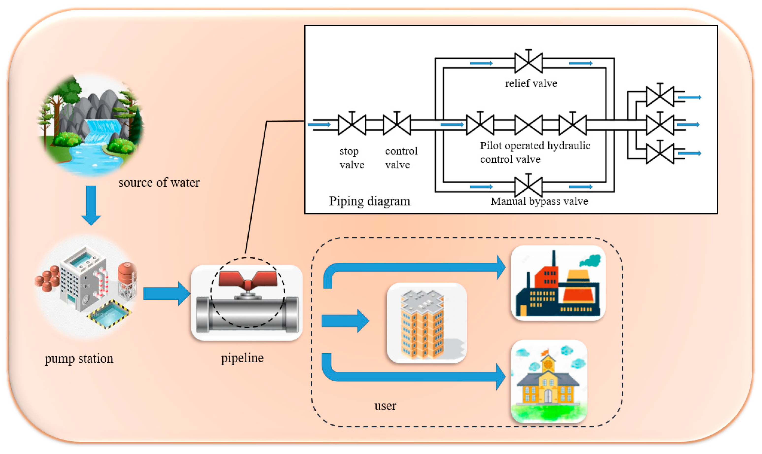
Figure 1: Urban water supply system diagram.
2.2 Mathematical Model of Urban Water Supply System Pipeline System
The analysis of the pipeline model is from the perspective of components. The analysis of the pipeline can be compared with the analysis of the electronic components in the circuit system, and the modeling of the fluid pipeline can be completed by means of the circuit theory. For the hydraulic pipeline with fixed diameter and axial laminar flow, it can be approximately equivalent to the transmission line. The schematic diagram of the distributed parameter model for the pipeline is shown in Fig. 2, where the pipeline is divided into numerous elements, each consisting of hydraulic resistance, capacitance, inductance, and conductance. Among them, R represents hydraulic resistance, C represents hydraulic resistance, L represents hydraulic capacitance, and G represents hydraulic conductance.
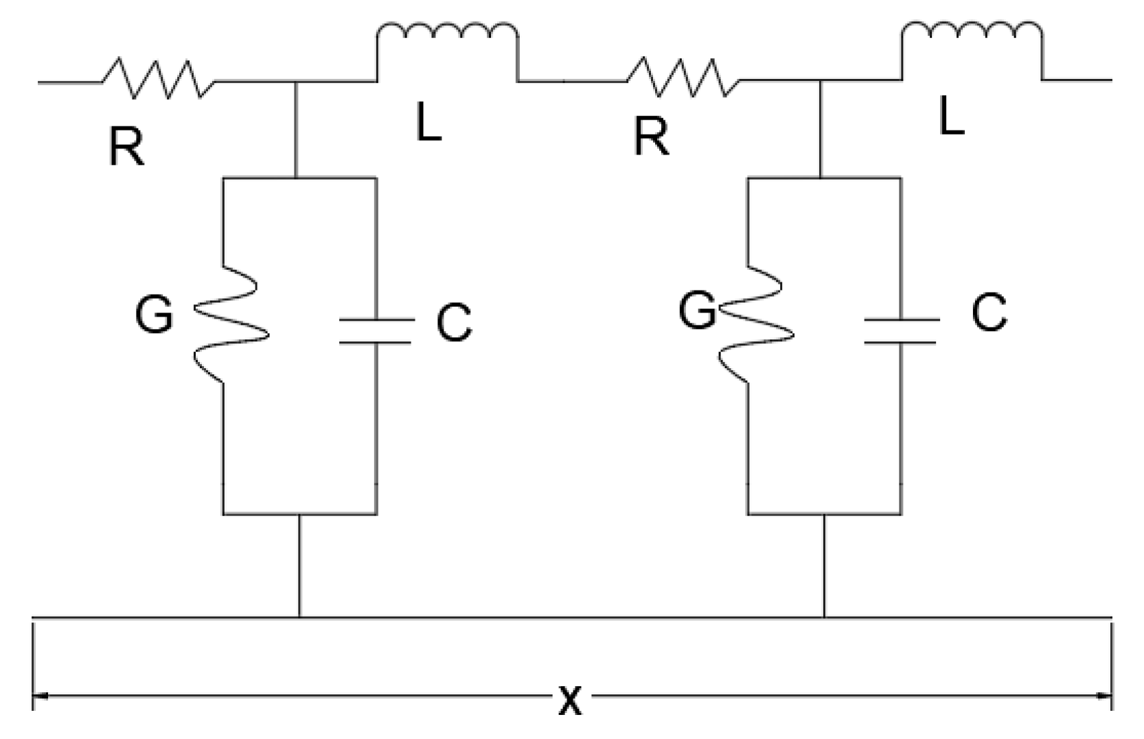
Figure 2: Piping distributed parameter model diagram.
q(x, t) and p(x, t) represent the instantaneous volume flow rate and pressure at any point on the pipeline, respectively.
From Kirchhoff voltage laws and Kirchhoff current law, it can be obtained that:
Dividing Eqs. (1) and (2) by Δx and taking the limit as Δx → 0 yields the system of Eq. (3):
Applying the Laplace transform to Eq. (3) with initial values of zero, we obtain:
Y(s) = G + Cs—Shunt admittance
P(x, s)—Laplace transform of p(x, t)
Q(x, s)—Laplace transform of q(x, t).
Taking partial derivative of an item in Eq. (4) to x, we can get:
Eq. (5) represents the wave equation. The propagation constant Y(s) is defined as:
The wave equation can be expressed as:
The general solution of Eq. (7) is:
Substituting into Eq. (4), we get:
At the input end where x = 0, P(x, s) = P1(s) and Q(x, s) = Q1(s), solve for the integration constants C1 and C2 and substitute them into (8) and (9) [20]:
At the end of the pipeline x = l, P(x, s) = P2(s), Q(x, s) = Q2(s), we get:
Organize the form (12) into a matrix:
Eq. (13) is the basic equation of the dynamic characteristics of the fluid transmission pipeline. The relationship between input and output can be evolved into different equations by the Eq. (13).
2.3 Mathematical Model of Pilot Hydraulic Valves
The adjustable system pressure range of the Pilot hydraulic valves is 0.7~1.6 MPa, with the valve outlet pressure consistently maintained at a lower value, and the flow design specification is 30 t/h.
According to the working principle of the pilot hydraulic control valve, the mathematical model has been simplified as follows:
- (1)Since the water supply pipeline model considers the influence of each pipeline component on the valve, the influence of each pipeline component on the front pressure in the valve dynamic model is ignored;
- (2)Due to the low compressibility of water, the influence of the medium on the dynamic characteristics of the valve is not considered in the model;
- (3)Since there are strict requirements for sealing during design, and the sealing structures such as diaphragms used in this product are good, internal and external leakage of the valve is not considered in the model.
The schematic diagram and principle diagram of the Pilot hydraulic valves are shown in Fig. 3.
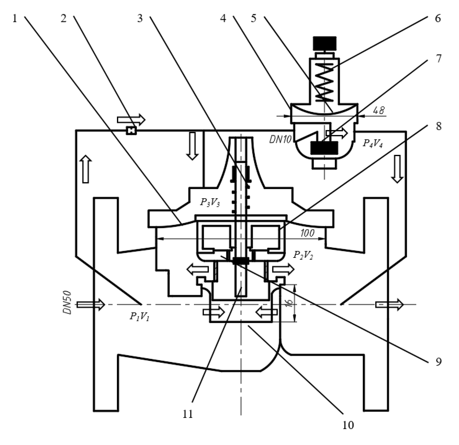
Figure 3: The schematic diagram and principle diagram of the Pilot hydraulic valves. 1. Main valve diaphragm. 2. Throttling element. 3. Main valve spring. 4. Pilot valve. 5. Pilot valve diaphragm. 6. Pilot valve spring. 7. Pilot valve core. 8. Diaphragm support. 9. Upper sleeve. 10. Lower sleeve. 11. Valve stem.
2.3.1 Establishment of Mathematical Model of Main Valve Motion Component
When the main valve spool is in motion, the forces acting on it along the axial direction mainly include: gravity, hydraulic differential force on both sides of the diaphragm, spring force, diaphragm resilience, friction force, and fluid viscous damping force. The force diagram of the main valve moving assembly of the Pilot hydraulic valves is shown in Fig. 4 [21].
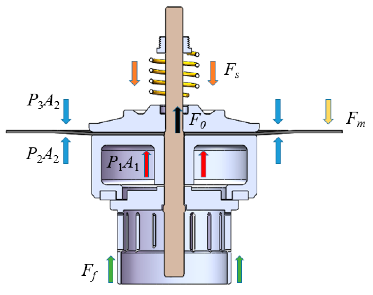
Figure 4: Pilot type hydraulic control valve main valve motion assembly force diagram.
The FP calculation formula of the fluid force in the motion direction of the main valve diaphragm is as follows:
P2—Main valve back pressure, Pa;
P3—Pilot valve chamber pressure, Pa;
A1—Main valve spool stress area, m2;
A2—Main valve diaphragm effective stress area, m2.
The formula for calculating the effective force area of the diaphragm is as follows:
dm1—Diaphragm top diameter, m;
Ds—Outer diameter of valve stem, m.
The main valve spring force Fs calculation formula is as follows:
K1—Main valve spring stiffness, N/m;
x1—Main valve spring pre-compression, m;
x—Main valve spool displacement, m.
The main valve hydraulic Fy calculation formula is as follows:
D—Main valve spool diameter, m;
Cd1—Valve port flow coefficient.
The formula for calculating the gravity Fg of the main valve motion component is as follows:
The main valve viscous damping coefficient B1 calculation formula is as follows:
Db1—Damping ring gap diameter, m;
L1—Relaxation length, m;
δ1—Circumferential gap, m.
The calculation formula of the friction force generated by the pre-compression of the O-ring is as follows:
do—O-ring section diameter, m;
Do—Outer diameter of O-ring, m;
eo—Compression ratio;
μo—Poisson’s ratio of nitrile rubber material;
Eo—Elastic modulus of nitrile rubber, Pa.
According to the Stribeck friction model, the friction force Ff between the stem and the filler can be expressed as:
Fs1—Maximum static frictional force, N;
vs—Stribeck speed, m/s.
Obviously, the friction model is discontinuous and non-differentiable at x = 0, which will bring trouble to the subsequent solution of the model. Therefore, the friction model is smoothed in this paper, that is, the continuous function is used instead of the symbolic function. The smoothed friction model is:
Differential equation of motion of Pilot hydraulic valves:
2.3.2 Establishment of Mathematical Model of Guide Valve Motion Component
When the pilot valve spool is in motion, the forces acting on it along the axial direction mainly include gravity, the differential hydraulic force across the diaphragm, spring force, diaphragm resilience, friction force, and viscous damping force of the fluid. The force diagram for the moving parts of the main valve of the Pilot hydraulic valves is shown in Fig. 5.
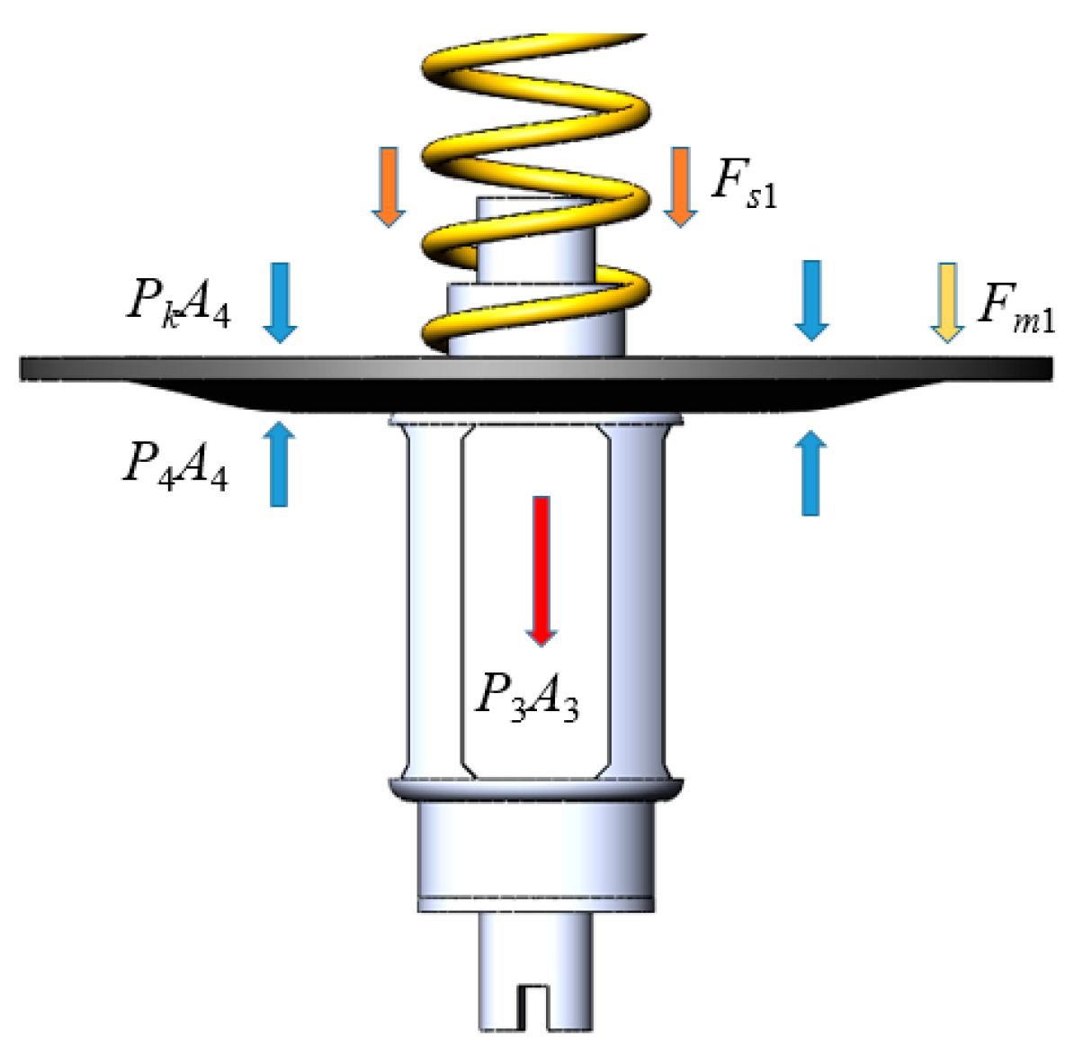
Figure 5: Force diagram of guide valve motion components of pilot hydraulic control valve.
The calculation formula of the fluid force FP1 in the motion direction of the guide valve diaphragm is as follows:
A4—Effective force area of guide valve diaphragm, m2;
Pk—Atmospheric pressure, Pa.
The formula for calculating the effective force area of the diaphragm is as follows:
dm2—Diaphragm top diameter, m.
The calculation formula of the guide valve spring force Fs1 is as follows:
K2—Guide valve spring stiffness, N/m;
y1—Guide valve spring pre-compression amount, m;
y—Guide valve spool displacement, m.
The calculation formula of the flow force Fy1 of the guide valve is as follows:
d0—Guide valve spool diameter, m.
The calculation formula of the gravity Fg1 of the guide valve moving component is as follows:
The calculation formula of the viscous damping coefficient B2 of the guide valve is as follows:
Db2—Damping ring gap diameter, m;
L2—Relaxation length, m;
δ2—Circumferential gap, m.
According to the structure and working principle of the pilot valve of the pilot hydraulic control valve, the force balance equation of the valve core is established.
2.4 Establishment of System Dynamics Model
The main parameters of the Pilot hydraulic valves are shown in Table 1.
Table 1: Main parameter values of pilot hydraulic control valve.
| Known Parameters | Symbol/Unit | Numerical Value |
|---|---|---|
| Main valve nominal diameter | DN | 50 |
| Main valve nominal pressure | PN | 16 |
| Main valve core sleeve diameter | D1/mm | 50 |
| Main valve diaphragm diameter | Dm1/mm | 100 |
| Main valve spring stiffness | K1/N·mm−1 | 12.2 |
| Main valve spring pre-compression | x0/mm | 10 |
| Total stroke of main valve core | x/mm | 16 |
| Diameter of pressure pipe | d/mm | 10 |
| Pilot valve spring stiffness | K2/N·mm−1 | 4 |
| Pilot valve spring pre-compression | y0/mm | 8 |
| Diameter of pilot valve diaphragm | Dm2/mm | 48 |
| Total travel of pilot valve core | y/mm | 10 |
| Bulk modulus of water | E/Pa | 2.09 × 10⁹ |
The fluid flow process of the Pilot hydraulic valves and the motion process of the main valve and the motion component of the pilot valve can be described by the above mathematical model. In order to clarify the relationship between the physical quantities and make the logic more smooth, the system dynamics model of the Pilot hydraulic valves is constructed in the form of transfer function, which provides theoretical support for the design improvement of the Pilot hydraulic valves and the subsequent establishment of the MATLAB/Simulink dynamic characteristic simulation model of the subsea tree hydraulic control system and the Pilot hydraulic valves.
Q1—Main valve flow, t/h;
Q2—Guide valve flow, t/h;
Q3—The flow through the spool sleeve, t/h;
Q4—Flow through the pressure pipe, t/h.
3 Dynamic Characteristics Analysis of Pilot Hydraulic Valves
3.1 CFD Turbulence Model Calculation and Flow Channel Meshing
The medium in the urban water supply system is mostly turbulent flow when passing through the pilot control valve, and the turbulence has strong randomness. Although the N-S equation is generally suitable for fluid flow, the turbulence state cannot be directly described at present, and a suitable turbulence model needs to be selected. In co-simulation, different turbulence models have their own advantages and disadvantages: large eddy simulation (LES) can analyze large-scale eddy structures and have high accuracy, but are expensive to calculate; direct numerical simulation (DNS) has the highest accuracy, but has a huge demand for computing resources, and is only suitable for low Reynolds’ simple flow; while the Renault average Navier-Stokes (RANS) model homogenizes the turbulent pulsation when passing through, which significantly reduces the computational complexity and is suitable for rapid simulation of high Reynolds’ flow in engineering, especially in steady-state or quasi-steady state problems. RANS has high computing efficiency and good stability. The widely verified turbulent enclosed models can meet the accuracy requirements of most engineering simulations, and are suitable for complex geometric or large-scale collaborative simulation scenarios. Therefore, the RANS method is selected to simulate the flow field of the pilot hydraulic control valve [22,23].
- (1)Governing equations of fluid mechanics
The continuity equation, as one of the fundamental equations in fluid mechanics, can be mathematically expressed as:
Introducing the Nabla operator, it can be written as:
u, v, w—The components of the velocity vector u in the x, y, and z directions;
u—Velocity Vector;
t—Time.
The momentum equation is based on the fundamental principle of Newton’s second law, and its mathematical equation in space can be represented in different directions as follows:
τxy, τyx, τzx—The component of viscous stress τ on the micro-element;
Fx, Fy, Fz—Forces acting on the infinitesimal element from the outside.
- (2)Turbulence equation
The flow velocity of the internal medium of the Pilot hydraulic valves is:
For the k-ε two-equation turbulence model, where the Reynolds averaged equation is:
μi—Turbulent viscosity of medium.
The equations of turbulent kinetic energy k and turbulent kinetic energy dissipation rate ε are:
In the formula, Pkb and Pεb represent the influence of buoyancy; Pk is the generation term of viscous force and buoyancy; the values of Cε1, Cε2, σk and σε are 1.44, 1.92, 1.0 and 1.3, respectively.
In the Fluent software’s solution settings, the Pressure-Implicit with Splitting of Operators (PISO) is used for pressure-velocity coupling, which can shorten the solution time. For numerical solution, the finite volume method is adopted, with the second-order upwind scheme for the convection term, the central difference scheme for the diffusion term, and the second-order implicit scheme for time discretization [24].
Mesh generation is an extremely crucial step in ensuring computational accuracy. The fluid model of the Pilot hydraulic valves selects unstructured grids and uses Mesh for division. The fluid in the front and rear pipes of the valve flange adopts hexahedral element grid, and the flow channel part of the valve in the middle of the pipe flange adopts tetrahedral element grid. The structure of the moving component and the fluid contact part is more precise. Therefore, the local refinement of the grid in this area makes the numerical simulation more accurate. Considering the influence of boundary layer, five layers of boundary layer are divided on the surface of valve body and pipeline. The height of the first layer grid is 0.46 mm, and the growth rate is 1.2. The grid division of the whole flow field is shown in Fig. 6 and Fig. 7.
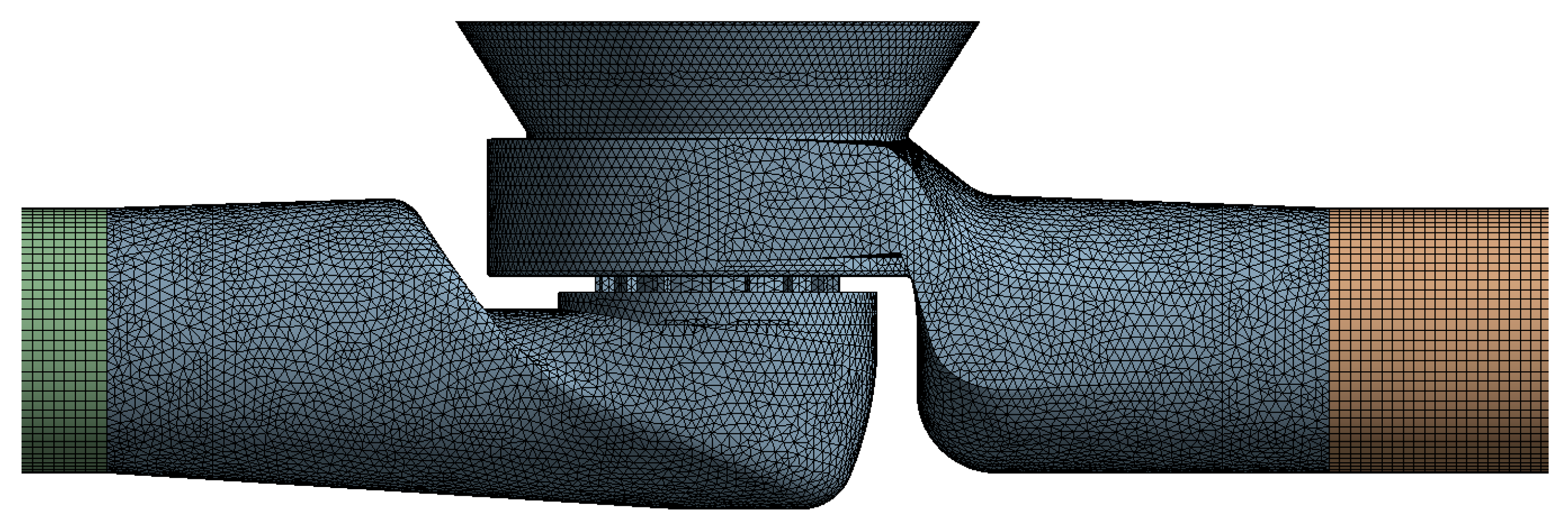
Figure 6: Model flow field meshing.
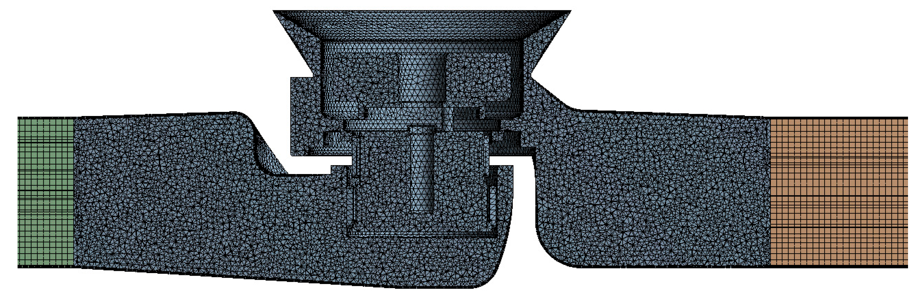
Figure 7: Grid division of internal flow field in the model.
The grid independence verification results in Table 2 indicate negligible variations in both flow rate and valve force between successive grid refinements, with flow rate changes of 0.24% (Grid 1 to Grid 2) and 0.12% (Grid 2 to Grid 3), and corresponding valve force fluctuations of 0.7% and 0.57%, respectively. With all force variations remaining below the 1% threshold and demonstrating clear convergence trends, while balancing computational accuracy with resource requirements, the numerical solution achieves grid independence at the mesh configuration of 514,270 nodes and 2,235,658 elements.
Table 2: Grid independence test.
| Mesh Type | Hop Count | Number Field of Element | Calculate the Flow Value (kg/s) | Valve Force (Pa) |
|---|---|---|---|---|
| Grid 1 | 342,795 | 1,575,826 | 8.30 | 6.87 × 10⁵ |
| Grid 2 | 514,270 | 2,235,658 | 8.32 | 6.92 × 10⁵ |
| Grid 3 | 872,538 | 2,693,512 | 8.33 | 6.96 × 10⁵ |
3.2 The Establishment of One and Three Dimensional Joint Dynamic Characteristic Simulation Model
Using the idea of one-dimensional and three-dimensional software interaction, the precise simulation characteristics of Fluent are used to supplement the simplified and neglected elements in the one-dimensional simulation model, and a high-precision dynamic characteristic collaborative simulation platform is established. The parameter transfer is realized by accessing the shared data file and modifying the relevant parameters in the Journal script file of Fluent by using the file Input/Output operation. MATLAB/Simulink can use the S function module data input and output interface function expansion, Fluent numerical simulation process will form a journal script file, with a certain amount of data and UDF function to realize the program interface function, complete with MATLAB/Simulink as the leading, Fluent as a collaborative module called by S function programming collaborative simulation platform. The specific implementation method and simulation process are shown in Fig. 8. Using Fluent, a fluid simulation software, as the 3D fluid simulation co-simulation component of the co-simulation platform, with the S-function serving as the interaction module between 1D and 3D software. The self-starting of Fluent is achieved through the “system” command line, and the simulation task for a specific number of steps is completed by reading the journal log file. Regarding the issue of data interaction in numerical simulations, there is no interface for MATLAB/Simulink and Fluent to mutually read each other’s data. Therefore, it is necessary to write the location for storing shared text and the reading commands in the S-function to enable the sharing of relevant parameters. Based on the simulation process shown in Fig. 7 and the design ideas for the co-simulation module mentioned above, the MATLAB/Simulink and Fluent co-simulation platform is designed as shown in Fig. 9, including the guide valve sub-module, the pressure sub-module of the system, the mechanical calculation sub-module of the main valve spool and the Fluent co-interface written by S function. The Fluent co-interface written by S function can read the valve flow obtained by Fluent simulation, the medium force monitoring results of the valve spool and diaphragm in the direction of valve spool movement, and the pressure value of each chamber of the main valve can be obtained by setting the monitoring points. As shown in Fig. 10, this is the data interaction relationship between the Fluent collaborative module of the collaborative simulation platform and the simulation main model. The Fluent collaborative module, as an independent module, obeys the call of the dynamic characteristics simulation main model.
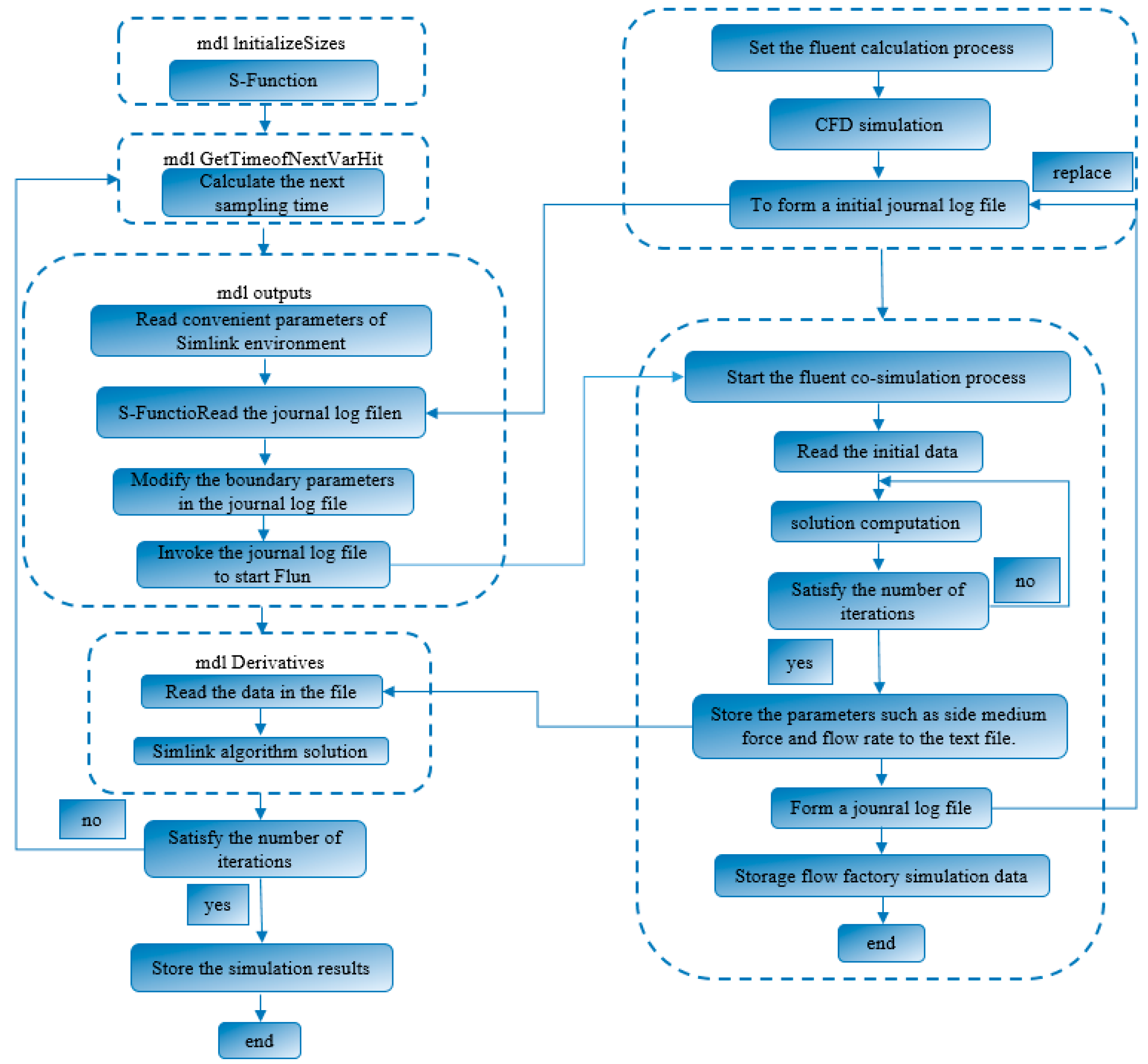
Figure 8: Implementation method of MATLAB/Simulink and Fluent co-simulation platform.
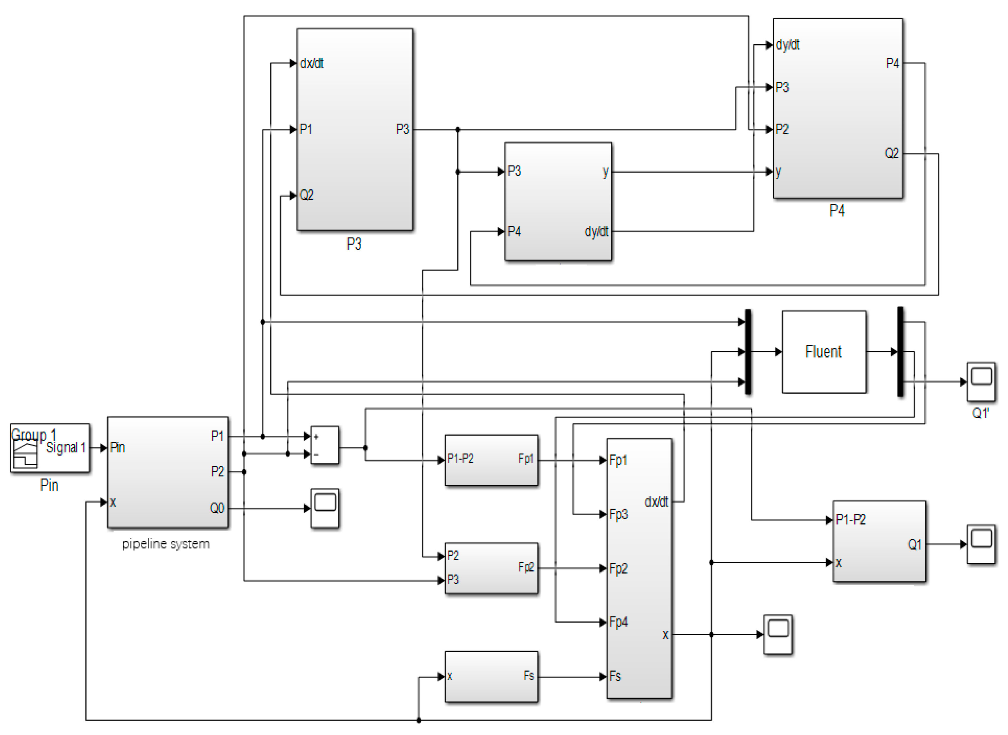
Figure 9: MATLAB/Simulink and Fluent co-simulation platform model.
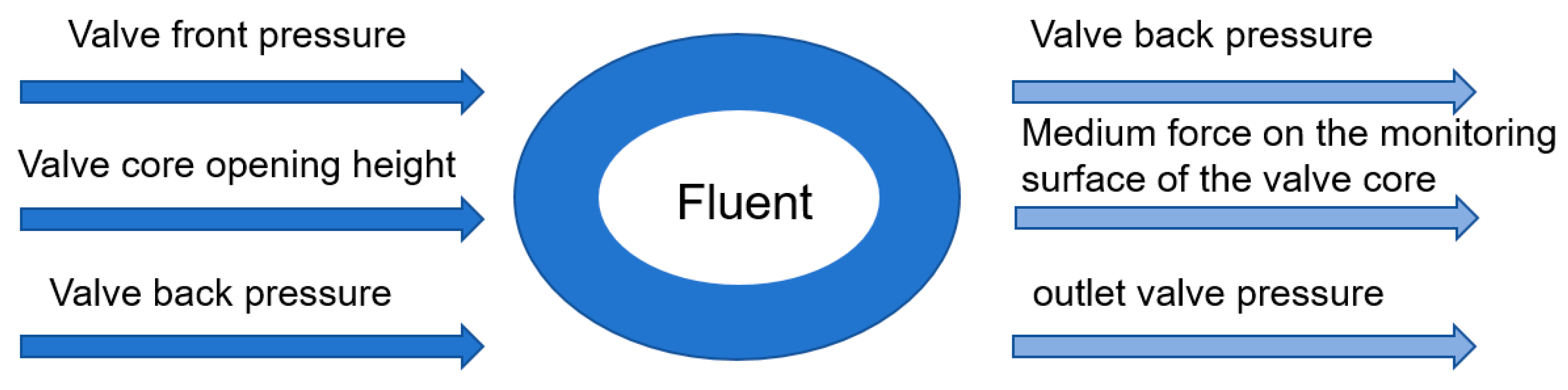
Figure 10: Fluent collaboration module in the collaborative simulation platform.
3.3 Co-Simulation Results and Analysis
The initial design parameters of the pilot hydraulic control valve are brought into the collaborative simulation platform. The given input signal is that the system inlet pressure changes from 0.7 MPa to 1.6 MPa. Through the MATLAB/Simulink model in the collaborative simulation platform, the displacement and velocity dynamic response curves of the main valve motion components under different system inlet pressures can be obtained.
As shown in Fig. 11, the response curves of the main valve motion components at different system inlet pressures are very similar. The displacement response curve tends to converge after three fluctuations. It can be seen from the figure analysis that the higher the system pressure, the smaller the opening of the hydraulic control valve, and the greater the starting speed of the main valve motion component. The numerical simulation results of fluid flow under different system inlet pressures by Fluent software are shown in Fig. 12, Fig. 13 and Fig. 14. The force of the calculated value of the main valve cavity pressure and the calculated value of the upper cavity pressure of the sleeve on the effective area in the simulation model is the key parameter affecting the opening of the main valve. In the Fluent fluid module of the collaborative simulation model, the force on the lower side of the diaphragm and the force on the upper side of the sleeve cavity can be directly monitored, thereby improving the simulation accuracy.
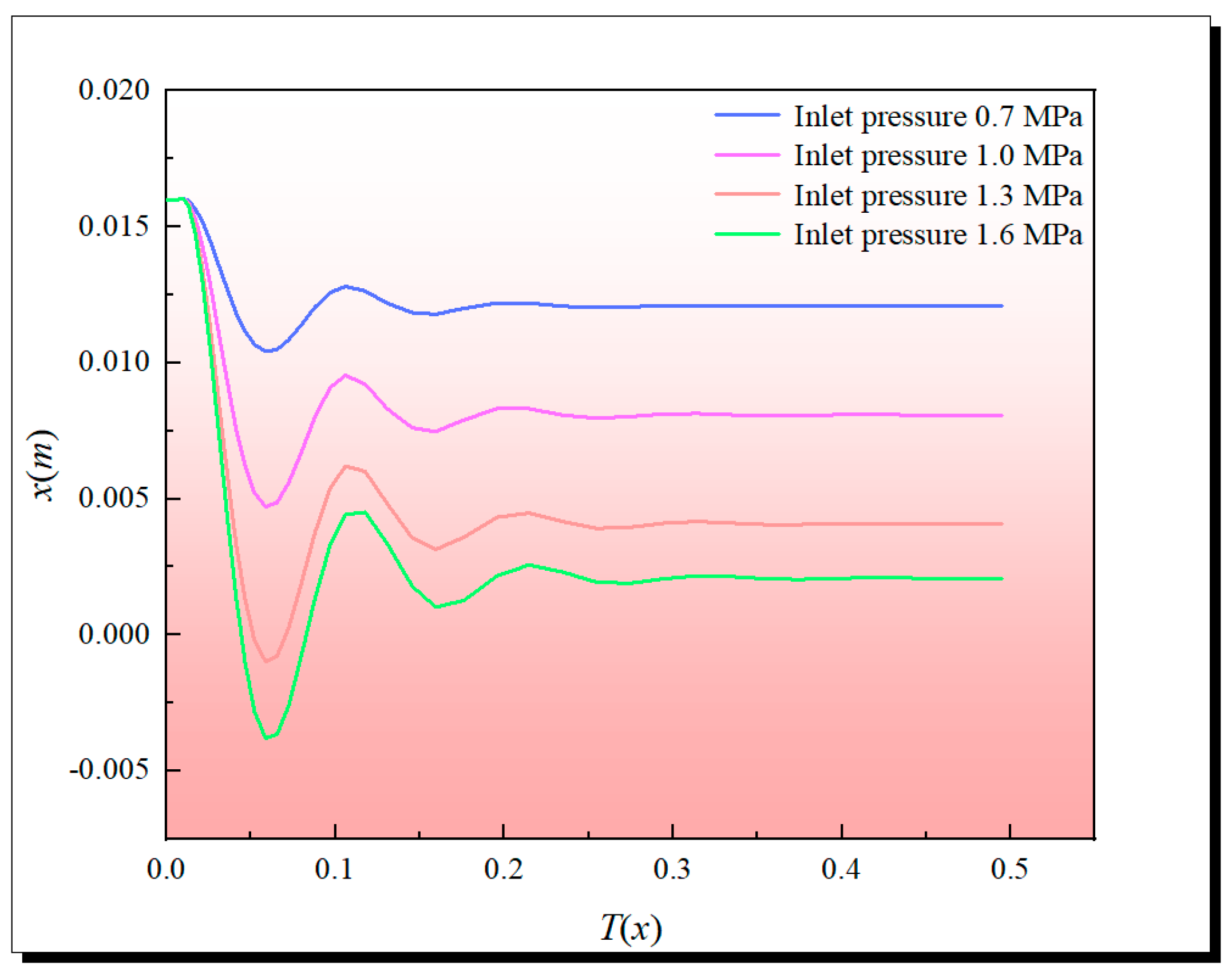
Figure 11: Displacement variation curve of main valve spool.
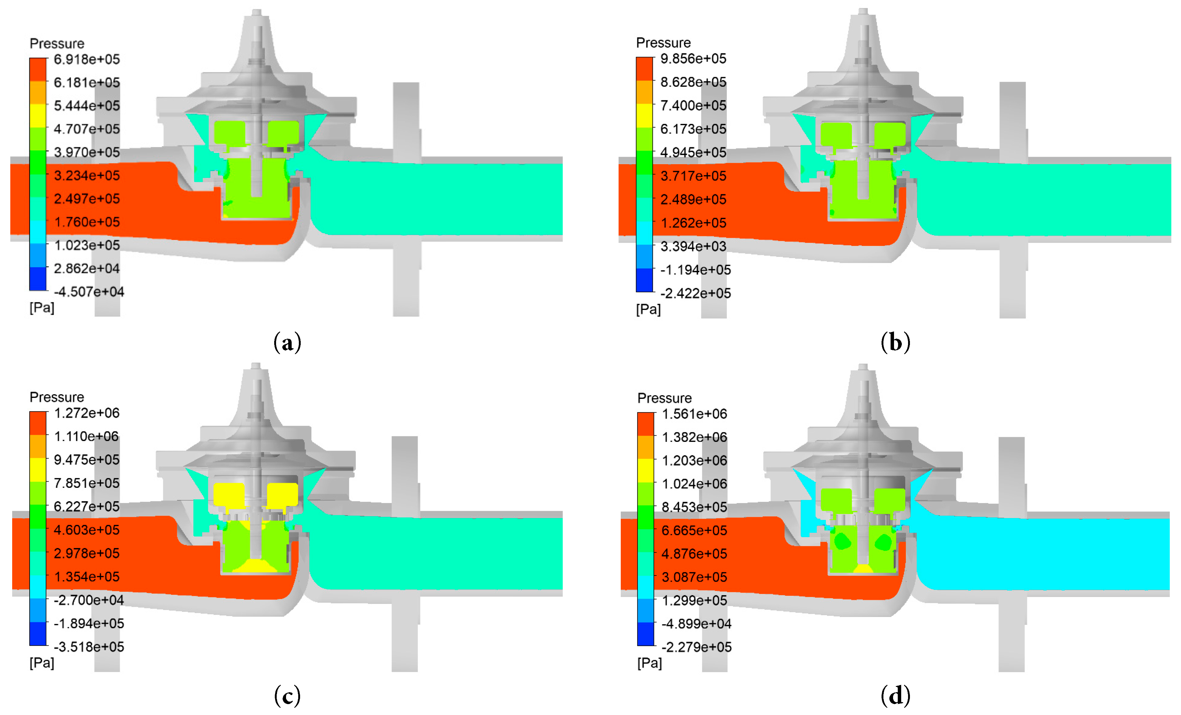
Figure 12: Pressure cloud diagram under different system inlet pressure. (a) Pressure 0.7 MPa; (b) Pressure 1.0 MPa; (c) Pressure 1.3 MPa; (d) Pressure 1.6 MPa.
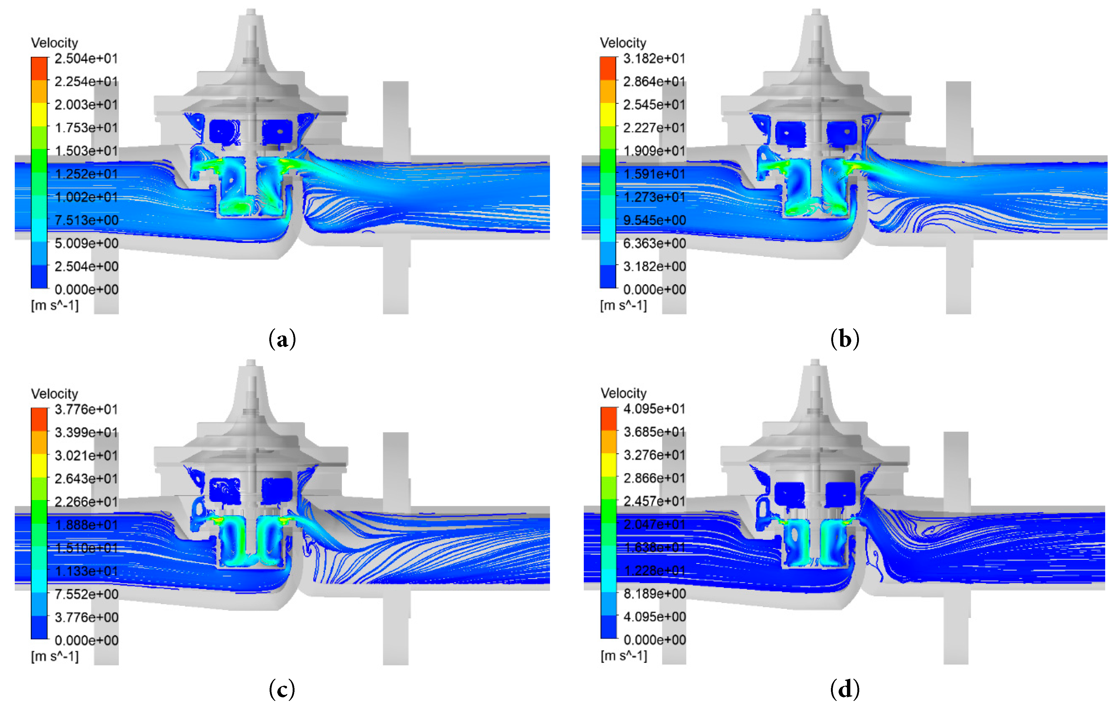
Figure 13: Velocity line cloud diagram under different system inlet pressure. (a) Pressure 0.7 MPa; (b) Pressure 1.0 MPa; (c) Pressure 1.3 MPa; (d) Pressure 1.6 MPa.
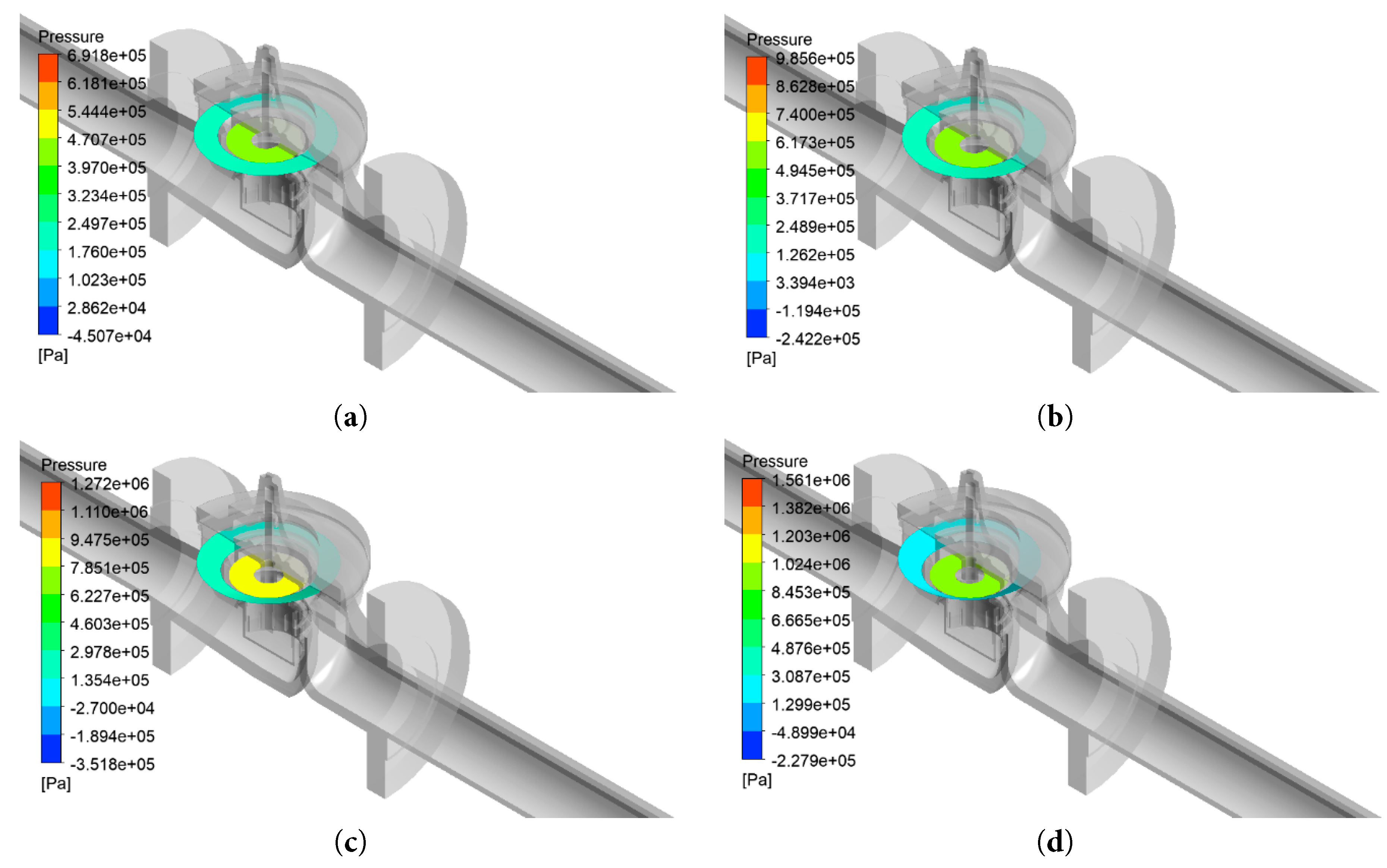
Figure 14: Monitoring surface medium force cloud diagram under different system inlet pressure. (a) Pressure 0.7 MPa; (b) Pressure 1.0 MPa; (c) Pressure 1.3 MPa; (d) Pressure 1.6 MPa.
According to the established simulation model of the dynamic characteristics of the water supply pipeline system, the input signal is given in the collaborative simulation platform. The inlet pressure of the system changes from 0.7 MPa to 1.6 MPa, and the hydraulic characteristics of the water supply pipeline and the pilot hydraulic control valve under different inlet pressures are simulated and analyzed. In the simulation model of the dynamic characteristics of the system, the inlet pressure of the system acts on the Pilot hydraulic valves after passing through the pressure drop of each flow resistance and pipeline in front of the valve. The analysis results are shown in Fig. 15. It can be seen that as the system inlet pressure increases, the system dynamic response time increases, and the system flow stability value increases. Compared with the design index of 30 t/h, the maximum flow deviation is 1.85 t/h, and the flow control accuracy is 6.17%, which does not meet the control accuracy. From Fig. 15, it can be seen that the flow deviation of the pilot hydraulic control valve is the largest when the inlet pressure of the system is 1.6 MPa. Therefore, the influence of different structural parameters on the dynamic characteristics of the system is studied when the inlet pressure of the system is 1.6 MPa.
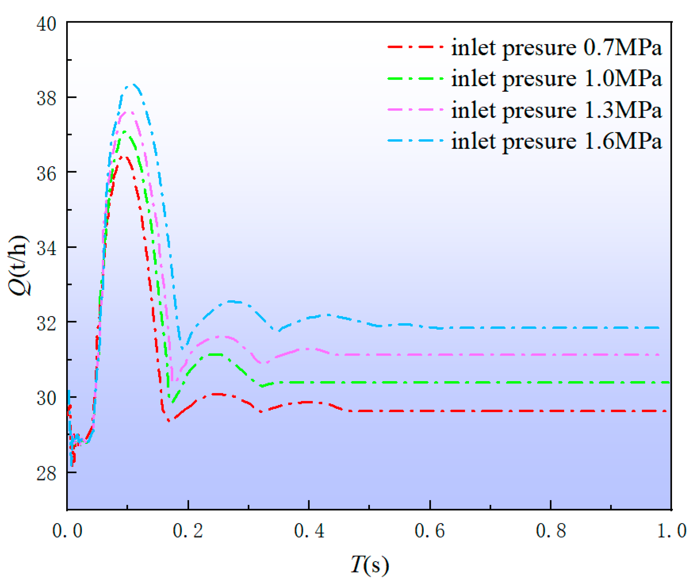
Figure 15: Flow diagram of different system inlet pressure system.
From Fig. 15, it can be seen that the flow deviation of the pilot hydraulic control valve is the largest when the inlet pressure of the system is 1.6 MPa. Therefore, the influence of different structural parameters on the dynamic characteristics of the system is studied when the inlet pressure of the system is 1.6 MPa. Through the constructed collaborative simulation platform, the dynamic characteristics of the Pilot hydraulic valves under different main valve spring stiffness are simulated and analyzed. The dynamic characteristic curves of the system with different structural parameters are shown in Fig. 16. The response time y1 of the dynamic characteristic curve exceeds 0.25 s, the overshoot y2 exceeds 38 t/h, and the stable value y3 exceeds 31.85 t/h. The relative difference with 30 t/h reaches 6.8%, which cannot meet the control accuracy requirements. Therefore, the original design of the valve performance is poor, need to be optimized.
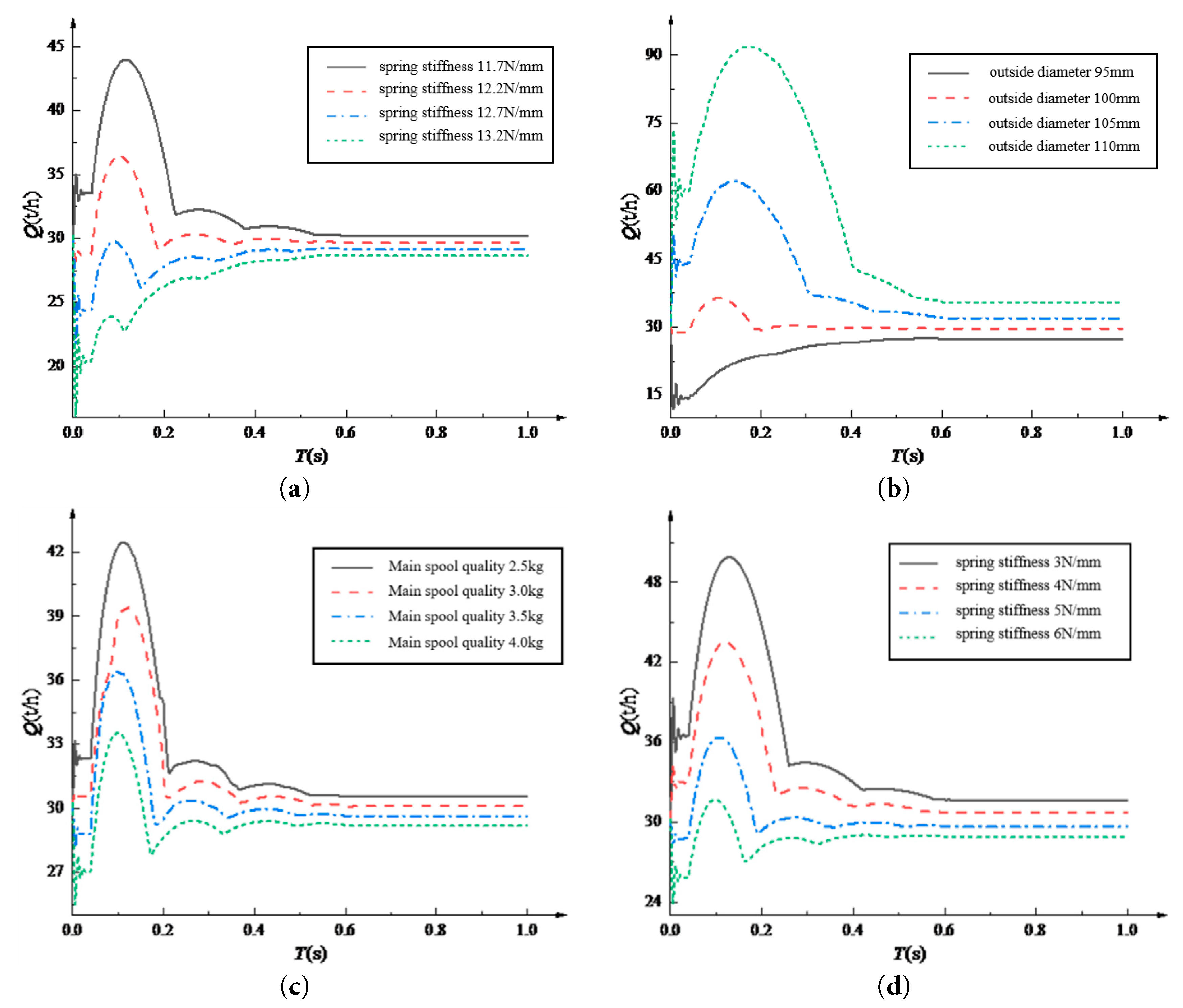
Figure 16: Flow dynamic characteristic curves of different structural parameters. (a) Dynamic characteristic curves of different main valve spring stiffness; (b) Characteristic curves of different diaphragm outer diameters; (c) The dynamic characteristic curves of different spool mass; (d) Dynamic characteristic curves of different pilot valve spring stiffness.
4 Multi-Objective Optimization Based on Surrogate Model
4.1 Defining Variables and Designing Experiments
As shown in Fig. 16, the main valve spring stiffness K1, the diaphragm outer diameter D1, the spool mass m and the pilot valve spring stiffness K2 of the pilot control valve are important parameters affecting the dynamic characteristics of the pilot valve, and the effect and degree of influence are different. The main valve diaphragm area and the pilot valve spring stiffness are the main parameters affecting the system flow. The main valve spring stiffness and the spool mass are the main parameters affecting the valve response time. The main valve spring stiffness and the main valve diaphragm area are the main parameters affecting the system overshoot. It is impossible to reduce the response time, overshoot and stability simultaneously by changing the value of a certain structural parameter. This is a typical multi-objective optimization problem.
The optimal Latin hypercube design has better uniformity, so that all sample points are evenly distributed in the design space as far as possible, which can better cope with the high correlation between input variables and generate more reasonable samples, thus improving the accuracy of simulation. The optimal Latin hypercube design method is used to combine the factor levels of the four variables shown in Table 3 to form the designed 50 scheme samples, and the response value of each sample point is calculated by the joint simulation method.
Table 3: Variable factor levels.
| Level | Factor | |||
|---|---|---|---|---|
| K1 (N·mm−1) | D1 (mm) | m (kg) | K2 (N·mm−1) | |
| −1 | 11.2 | 90 | 2.4 | 2 |
| 0 | 12.2 | 100 | 3.2 | 4 |
| 1 | 13.2 | 110 | 4.0 | 6 |
4.2 Improved Whale Algorithm to Optimize BP Neural Network (L-TIWOA-BP) Surrogate Model
4.2.1 Improved Whale Algorithm (L-TIWOA)
The whale optimization algorithm (WOA) was proposed in 2016, which was inspired by the special ‘bubble-net’ group predation strategy of humpback whales in nature [25]. In the WOA setting, the position of each whale represents a feasible solution. During the group predation process, each individual has three behaviors: randomly searching for prey, identifying the location of prey and encircling it, and using bubble nets to attack prey. Suppose that the position X of each whale in the n-dimensional solution space is:
When attacking prey (p ≥ 0.5), in order to form a bubble net, the whale swims to the prey in a spiral motion. Its position update formula is:
b—Constants defining the shape of the helix;
l—Random numbers distributed within [−1, 1].
When the prey is surrounded (p < 0.5), the whale decides to perform a contraction to surround the prey or randomly search the prey according to the size of A. When |A| < 1, the whale will swim to the individual with the best position to approach the prey. Its position update formula is:
When |A| ≥ 1, the whale will also randomly look around for prey, randomly select an individual in the group and approach it, its location update formula is:
A and C are coefficients, and the calculation formula is as follows:
a—Linear convergence factor.
The advantage of WOA is that the operation is simple and easy to implement, and there are fewer parameters to be adjusted, but it is a random generation of initial population. This method has low search efficiency, weak global search ability, and is easy to fall into local optimal solution. In order to solve the above problems, this paper adds Logistic-Tent (L-T) chaotic map to initialize the population, so that the population is more evenly distributed in the search space. Combined with adaptive weights, a nonlinear decreasing adaptive sine factor w is introduced to update the individual position of the whale.
The expression of L-T chaotic map is as follows:
A nonlinear decreasing adaptive sinusoidal factor w is introduced, which can satisfy the complex nonlinear variations in the WOA optimization process, and therefore, the positions of individual whales are updated as follows:
4.2.2 L-TIWOA optimized BP Neural Network
BP neural network is one of the most widely used machine learning models. Its structure is shown in Fig. 17, which includes three parts: input layer, hidden layer and output layer. Each layer of neuron nodes is fully connected with the adjacent layer of neuron nodes. BP neural network has a strong self-learning ability, which can grasp and store the mapping relationship between input and output data without knowing the mathematical equations that represent this mapping relationship in advance. However, in practical applications, BP neural network algorithm has the problems of slow convergence speed and easy to fall into local optimal solution. In order to solve these problems, L-TIWOA with global optimization ability is used to optimize the initial weights and thresholds of BP neural network, so as to reduce the possibility of falling into local optimal solution and improve the convergence speed and prediction accuracy of the network. The flow chart of L-TIWOA-BP is shown in Fig. 18.
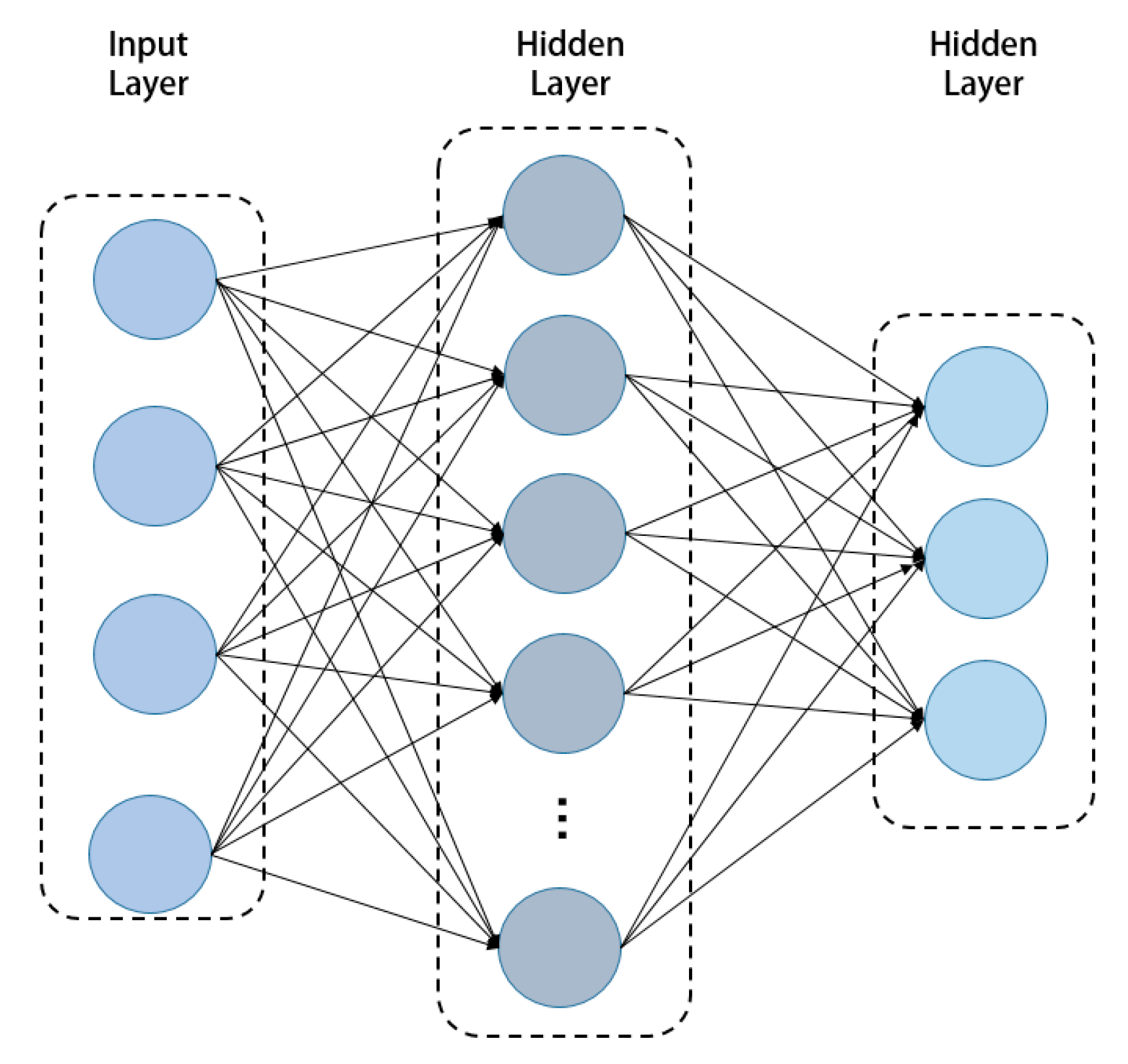
Figure 17: BP neural network structure.
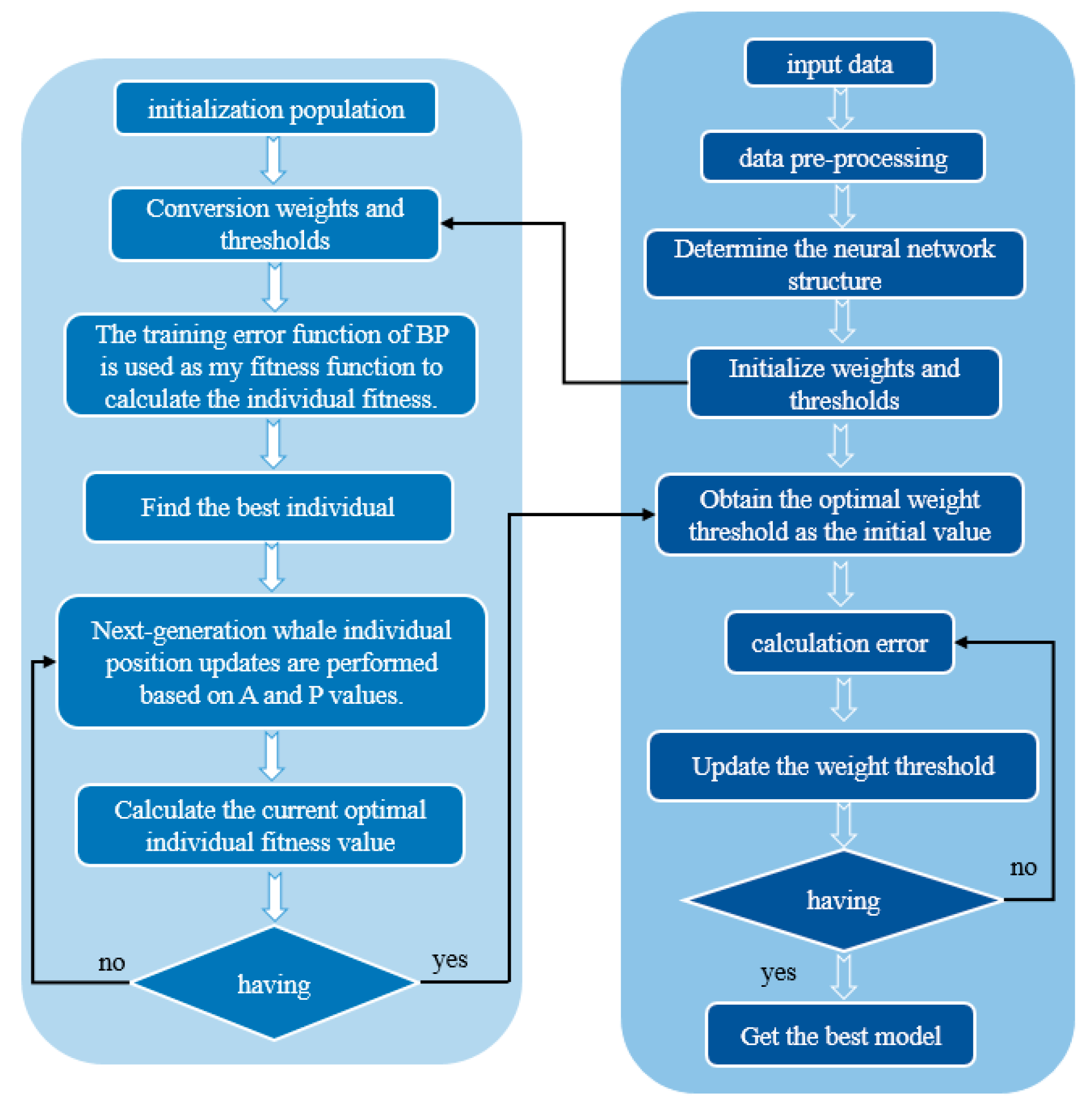
Figure 18: Flow chart of BP neural network optimized by L-TIWOA.
The comparison of output effects between the L-TIWOA-BP predicted values, the original BP predicted values, and the true values is shown in Fig. 19a,c,e. The L-TIWOA-BP predicted values are much closer to the true values than the original BP predicted values. The error comparison between the L-TIWOA-optimized BP neural network and the original BP neural network is shown in Fig. 19b,d,f. The prediction error of the BP neural network optimized by L-TIWOA is much smaller than that of the original BP neural network. As shown in Fig. 19, the L-TIWOA-BP surrogate model improves prediction accuracy compared to the original BP surrogate model and is more suitable for simulation optimization.
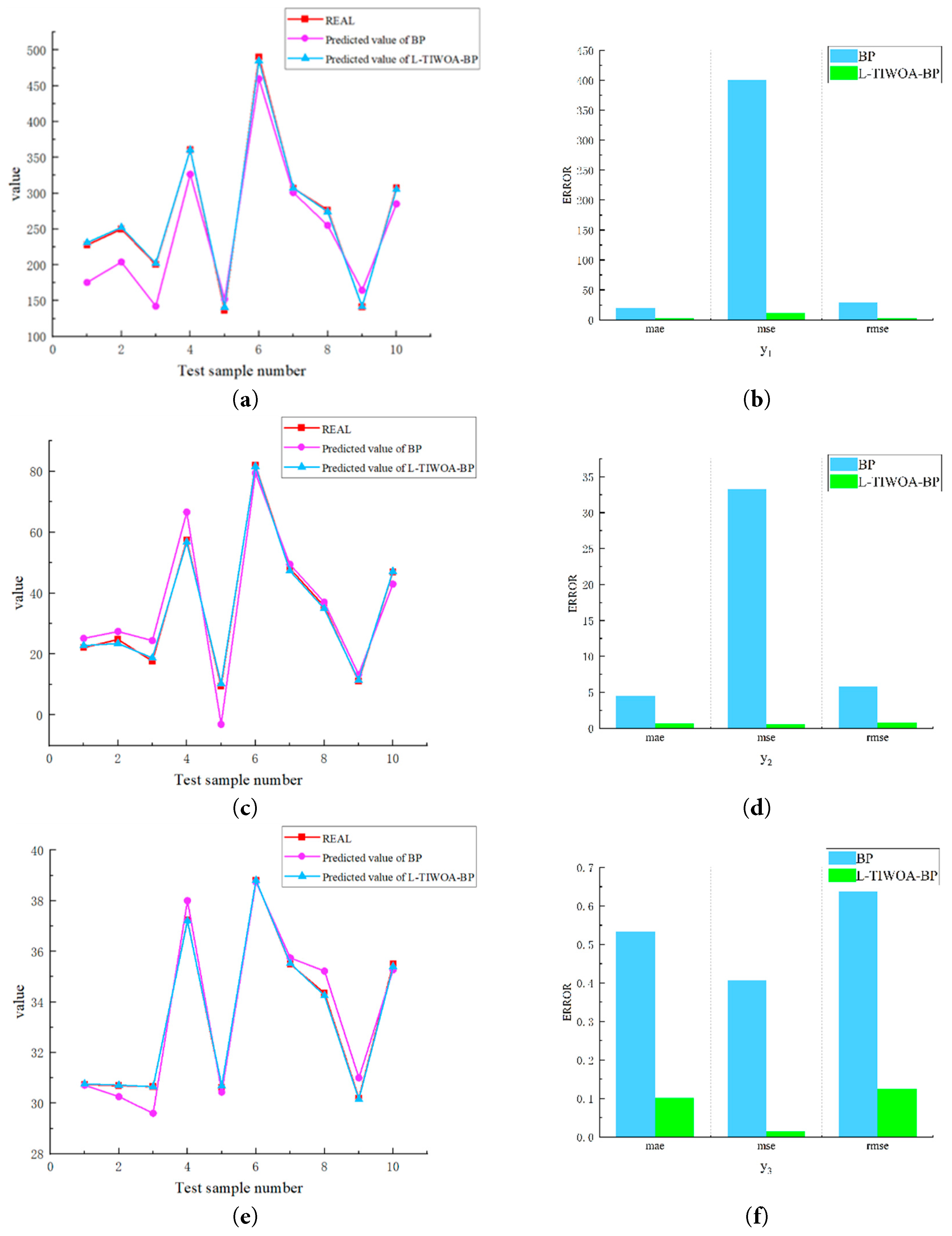
Figure 19: (a,c,e) Comparison of output effects between the L-TIWOA-BP predicted values, the original BP predicted values, and the actual values; (b,d,f) The error comparison between the optimized L-TIWOA BP neural network and the original BP neural network.
4.3 Multi-Objective Coati Optimization Algorithm (COA)
MOCOA is an optimization algorithm that optimizes multiple targets simultaneously on the basis of retaining COA’s efficient optimization. Although the basic single-objective COA of MOCOA has better optimization effect, for complex optimization problems, COA still has problems such as poor population diversity and insufficient local search ability. In order to improve the optimization performance of MOCOA, an improved multi-objective raccoon optimization algorithm is proposed [26].
The raccoon algorithm mainly consists of two stages: the exploration stage that simulates the hunting process of the coati to the iguana; the exploration stage that simulates the hunting process of the coati to the iguana.
In the multi-objective raccoon optimization algorithm, the initial population is first generated. After analysis, the initial population generated by COA in a random manner will lead to insufficient population ergodicity in the early stage of algorithm optimization, and it is difficult to effectively obtain high-quality information in the solution space, and the population diversity in the later stage will decrease, and it is easy to fall into local optimum. Therefore, this paper uses the Tent chaotic mapping method to initialize the population, increase the uncertainty, unrepeatability and unpredictability of the population, and generate uniformly distributed initial particles to increase the coverage of the population. The formula is as follows:
Exploration stage: Suppose an iguana is resting on a tree, and a group of coati intends to hunt the iguana. First, half of the coati began to creep up the treetops, forcing the iguana to fall to the ground. The process of climbing a tree is as follows:
Front1,j—The position of the j-th dimension of the iguana.
Inspired by the particle swarm optimization algorithm, an adaptive inertia weight strategy is adopted. When the coati is close to the prey, the smaller adaptive weight changes the position of the optimal coati and enhances the local optimization ability of the coati. The formula of adaptive weight is as follows:
The adaptive inertia weight is used to update xi,j, and the updated is
Development phase: When predators attack the raccoon, the raccoon will flee its position. Therefore, the raccoon position update formula in the development phase is as follows:
ubj, lbj—Local upper and lower limits in the j-th dimension.
The research shows that compared with the current solution, the reverse solution has a greater probability of approaching the global optimum. Therefore, this paper uses the reverse learning strategy to improve the optimization performance of COA, that is, the reverse learning strategy is applied to the location update of coati individuals to avoid the algorithm falling into local optimum. The reverse learning strategy formula is as follows:
k—Scaling factor.
After two stages, the newly completed individual is the offspring, and the individual before the update is the parent. The updated parent individual is merged with the offspring individual, and the fast non-dominated sorting is performed together, and the non-dominated frontier Frontl, l = 1, 2, …, K under each level is determined. Finally, the crowding distance of each raccoon in Frontl is calculated. The calculation formula of multi-target crowding distance is as follows:
M—Number of objective functions.
Select a new population, the selection process is as follows:
P0—Set of selected solutions.
When the number of individuals in the set is less than N, successively add the front individuals of Frontl to P0. When |P0 + Frontl| > N, select individuals with the largest values based on the crowding distance until the number of individuals in P0 is N.
Compared to the traditional multi-objective Coati algorithm, the improved version alters the population initialization method, increasing the uncertainty, non-repetitiveness, and unpredictability of the population. Generating uniformly distributed initial particles enhances population coverage and diversity. It adopts an adaptive inertia weight strategy to strengthen the raccoon’s local search capability and avoid falling into local optima. The flow chart based on the improved multi-objective raccoon algorithm is shown in Fig. 20.
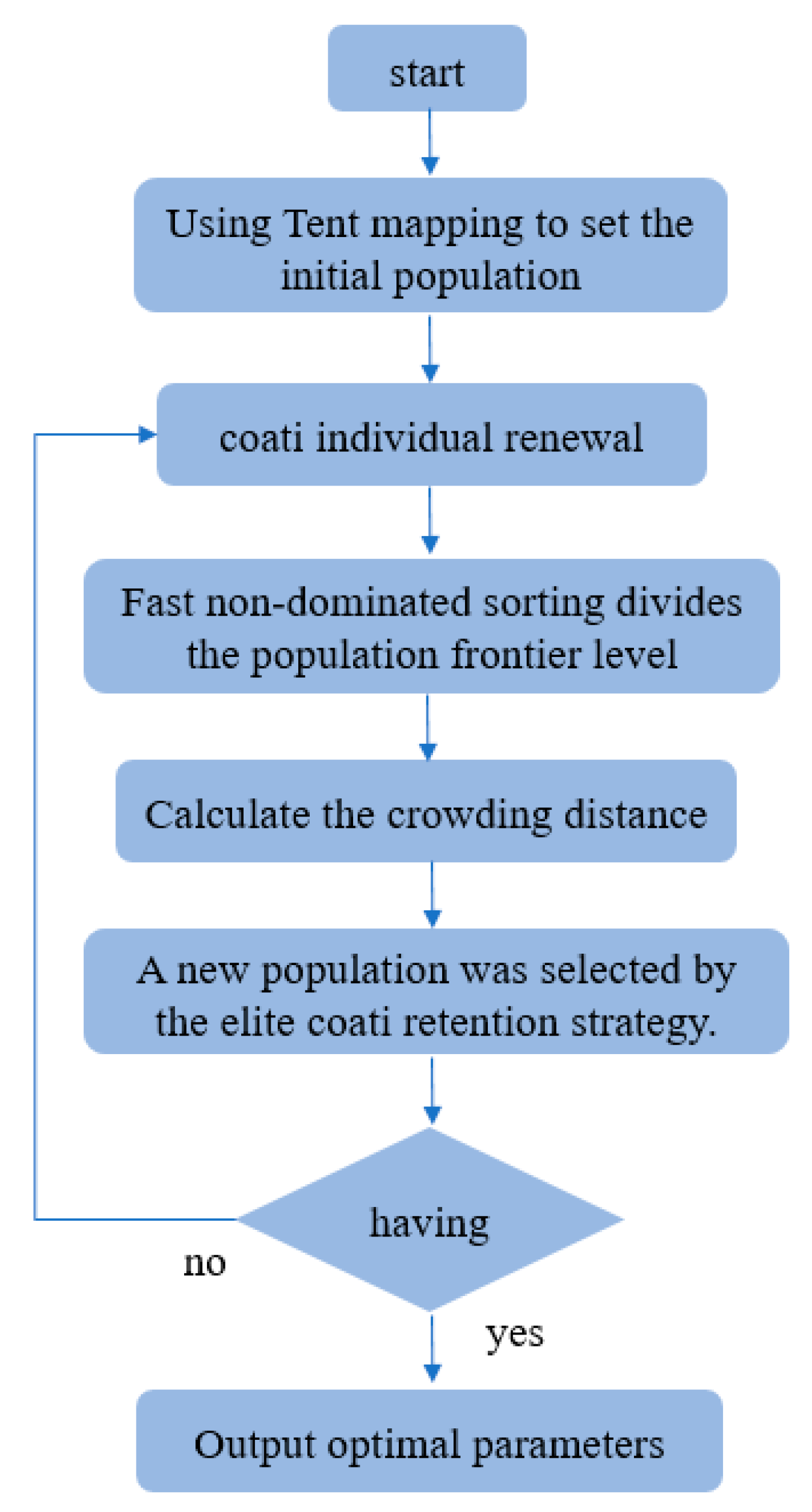
Figure 20: Improved multi-objective raccoon algorithm flow chart.
The L-TIWOA optimized BP neural network is used as the surrogate model. The Pareto front solution set of the improved MOCOA for the pilot hydraulic control valve optimization problem is shown in Fig. 21. The points in the figure represent the response values of the objective function of a set of design schemes. It can be seen that there is a certain distribution difference in the advantages and disadvantages of the response values of the three objective functions, and there is no design scheme with the three indicators all optimal.
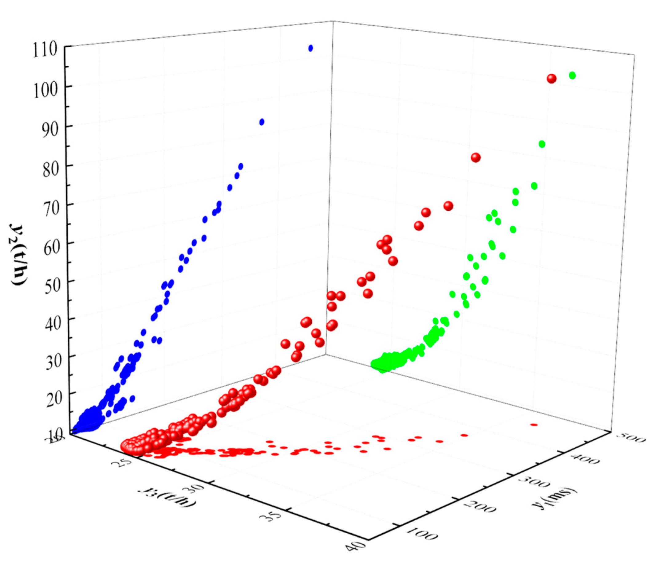
Figure 21: Pareto front solution set diagram.
According to the Pareto frontier solution set in Fig. 19, scheme A with the shortest flow response time, scheme B with the smallest response peak and scheme C with the closest flow to the design index can be obtained. Considering the design schemes of the pilot hydraulic control valve, the optimal combination of structural parameters is obtained. The evaluation indexes of each scheme are shown in Table 4. After optimization, the indexes of the valve are optimized to varying degrees, indicating that the improved algorithm has good effectiveness.
The optimal structural parameter combination of the Pilot hydraulic valves obtained through a multi-objective optimization algorithm is as follows: main valve spring stiffness of 12.5 N/mm, main valve diaphragm outer diameter of 98 mm, main valve spool mass of 3.8 kg, and pilot valve spring stiffness of 4.2 N/mm. Replace the corresponding structural parameters in the collaborative simulation platform, and use the platform to perform dynamic characteristic numerical simulation on the optimized valve. As shown in Fig. 22, the response peak of the optimized pilot-operated hydraulic control valve is significantly reduced, the response time is shortened, the stable flow rate is closer to the design specifications, and the flow control accuracy is greatly improved.
Table 4: Comparison of evaluation indexes before and after optimization.
| Compute | Structural Parameter | Required Value | |||||
|---|---|---|---|---|---|---|---|
| K1 (N/mm) | D1 (mm) | m (kg) | K2 (N/mm) | y1 (ms) | y2 (t/h) | y3 (t/h) | |
| A | 13.2 | 92.10 | 3.69 | 5.72 | 58.61 | 9.75 | 24.23 |
| B | 12.8 | 90.74 | 3.57 | 6 | 59.17 | 9.52 | 23.97 |
| C | 11.33 | 95.56 | 3.85 | 4.03 | 254.28 | 43.75 | 30.05 |
| initialization value | 12.2 | 100 | 3.5 | 4 | 226.8 | 38.35 | 31.75 |
| optimized | 12.5 | 97 | 3.8 | 4.2 | 178.5 | 36.20 | 29.94 |
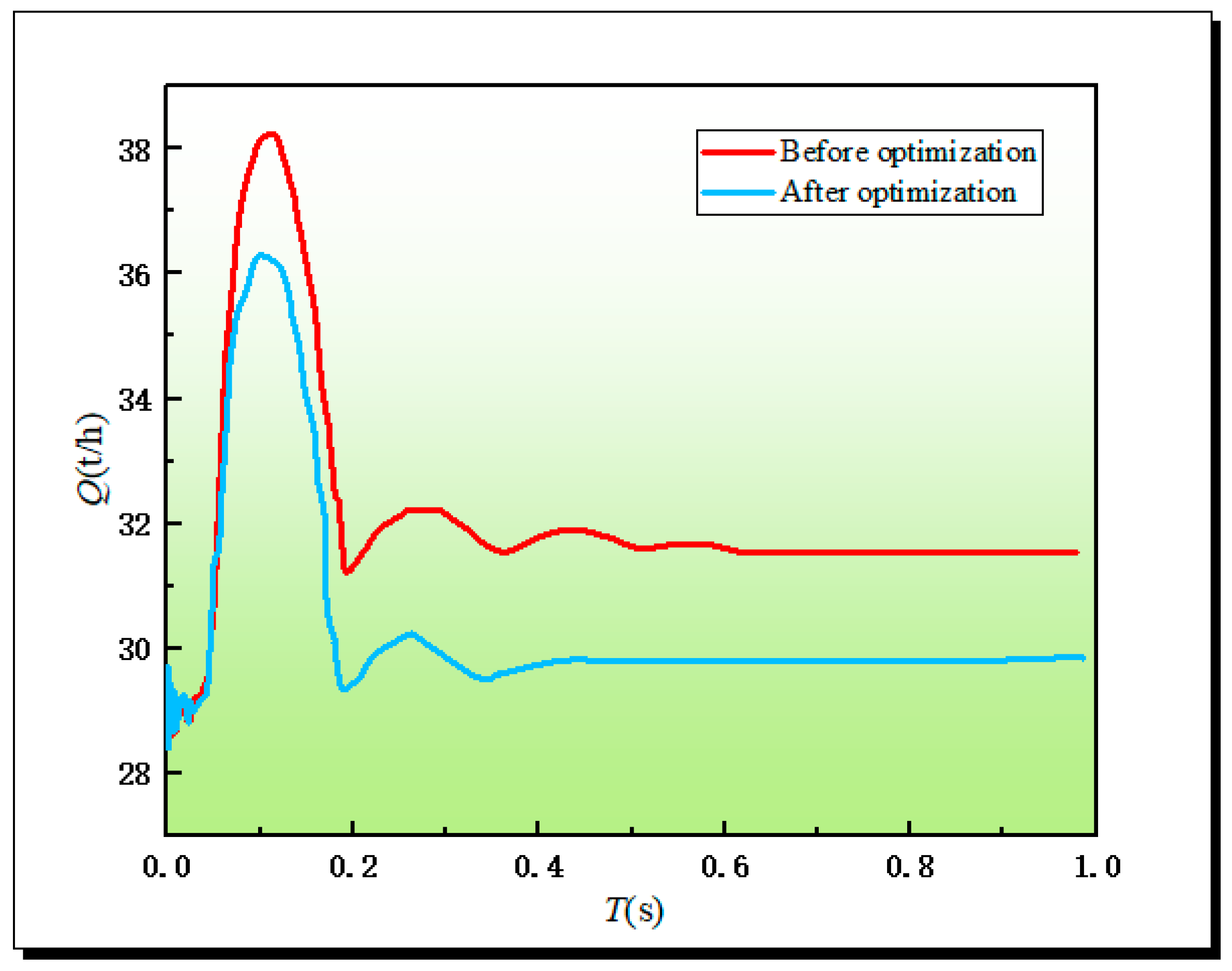
Figure 22: Comparison of dynamic characteristics of Pilot hydraulic valves before and after optimization.
4.4 Algorithm Complexity Analysis
This study conducted a calculation complexity analysis for cases containing 4 design parameters (D = 4) and 3 optimization goals (response time, flow bias, and overshoot).
In terms of proxy model, a BP neural network with 4 input nodes, 16 hidden layer neurons and 3 output nodes is used, which contains about K = 100 trainable parameters (hidden layer 4 × 16 weight + 16 bias; output layer 16 × 3 weight + 3 bias). Its prediction complexity is O(K × M) = O(300) floating point operations/time, because the output value of three targets needs to be calculated simultaneously.
The complexity of the Improved Multi-Objective Raccoon Optimization Algorithm (IMOMLOA) primarily stems from the non-dominated sorting operation, which requires O(M × N2) = O(3 × 2500) = O(7500) comparisons per generation (with a population size N = 50). By incorporating a surrogate model pre-screening mechanism, the number of high-fidelity simulation calls (each taking approximately 10 min) has been reduced from over 1000 to 200 selected evaluations.
Experimental results demonstrate the method’s good computational efficiency:
Total optimization time: approximately 30 h
Surrogate model prediction error: RMSE < 5% on the test set
Final solution quality:
Flow control accuracy: 3.7% deviation
Pressure overshoot: <5% of the set value
Response time: ≤0.2 s
The analysis confirms that, although the three objectives increase the theoretical complexity, the optimization framework based on the surrogate model effectively achieves multi-objective optimization while maintaining computational feasibility.
Aiming at the problem that the existing hydraulic control valve has insufficient flow and pressure regulation ability in a wide range of system pressure, a Pilot hydraulic valves with wide adjustable pressure range, high flow control accuracy, and anti-turbulence and cavitation is improved and designed. By investigating the research progress of domestic and foreign scholars in the research methods of dynamic characteristics of self-operated valves and multi-objective optimization algorithms, the numerical simulation research and multi-objective optimization of the dynamic characteristics of Pilot hydraulic valvess are carried out. The main conclusions are:
- (1)The mathematical model of urban water supply system pipeline is established by introducing the electrohydraulic simulation method, which provides theoretical support for the design improvement of pilot hydraulic control valve and the subsequent establishment of MATLAB/Simulink dynamic characteristics simulation model of pilot hydraulic control valve in urban water supply system pipeline.
- (2)By studying the internal flow of the valve in the dynamic characteristics simulation platform, a high-precision dynamic characteristics numerical simulation method considering both one-dimensional system and three-dimensional flow is developed, and a collaborative simulation platform is established. The simulation results show that as the system inlet pressure increases from 0.7 MPa to 1.6 MPa, the main valve opening gradually decreases, and the stable system flow increases from 29.65 t/h to 31.85 t/h. Compared with the design index of 30 t/h, the maximum deviation is 1.85 t/h, and the flow control accuracy is 6.17%, which does not meet the design requirements of ±5% control accuracy. The valve needs to be optimized.
- (3)Logistic-Tent (L-T) chaotic map and adaptive sine factor are introduced to optimize WOA algorithm, which improves the search ability of WOA algorithm. The L-TIWOA algorithm with global search ability is used to optimize the BP neural network, which improves the fitting accuracy and stability of the traditional BP model. Tent chaotic map, adaptive weight and reverse learning strategy are introduced to optimize MOCOA, which enhances the global and local search ability of the algorithm and avoids falling into local optimal solution.
- (4)The L-TIWOA-BP neural network is used to construct the surrogate model of the processing optimization target value and serve as the fitness function of the multi-objective optimization model. The improved MOCOA algorithm is used to iteratively solve the multi-objective optimization model. The optimal parameter combination of the pilot hydraulic control valve is: the spring stiffness of the main valve is 12.5 N/mm, the outer diameter of the main valve diaphragm is 97 mm, the mass of the main valve spool is 3.8 kg, and the spring stiffness of the guide valve is 4.2 N/mm. The optimal solution set is substituted into the collaborative simulation platform for simulation. The maximum flow deviation value is 1.11 t/h, and the flow control accuracy is 3.7%, which meets the design requirements of 5% flow control accuracy. It can be seen that the flow control accuracy is improved by 2.13% compared with that before optimization. The optimized pilot hydraulic control valve improves the stability and control accuracy of the system.
The Pilot hydraulic valves can be regarded as a nonlinear dynamic system with real-time varying parameters in the water supply pipeline system. When the input signal fluctuates or the system is disturbed, the stability of parameters such as displacement and pressure changes accordingly, leading to unstable flow regulation of the valve. The force balance state of the moving components is disrupted, resulting in instability phenomena such as vibration. Section 3 investigated various performance indicators of the dynamic characteristics of the Pilot hydraulic valves using a co-simulation platform. However, due to differences in theoretical methods and numerical simulation software, the stability of its dynamic system was not analyzed. Analyzing the bifurcation characteristics and stability of the dynamic system can be a future direction. In addition, future research will incorporate systematic comparisons with newly proposed optimization algorithms in recent years to further validate the universal applicability of the proposed optimization algorithm.
Acknowledgement:
Funding Statement: Gansu Provincial Department of Education (Industrial Support Plan Project: 202CYZC-048).
Author Contributions: Shuxun Li made contributions through review, modification, amendment, supervision. Xinhao Liu was responsible for the design of the work plan, numerical simulation, data analysis, chart drawing, and article writing. Yu Zhang performed data review and guidance. Yu Zhao revised and supervised the article. All authors reviewed the results and approved the final version of the manuscript.
Availability of Data and Materials: The datasets generated and/or analyzed during the current study are available from the corresponding author on reasonable request.
Ethics Approval: Not applicable.
Conflicts of Interest: The authors declare no conflicts of interest to report regarding the present study.
References
1. Shadloo MS , Oger G , Le Touzé D . Smoothed particle hydrodynamics method for fluid flows, towards industrial applications: motivations, current state, and challenges. Comput Fluids. 2016; 136: 11– 34. doi:10.1016/j.compfluid.2016.05.029. [Google Scholar] [CrossRef]
2. Alberto MB , Jesús Manuel FO , Andrés MF . Numerical methodology for the CFD simulation of diaphragm volumetric pumps. Int J Mech Sci. 2019; 150: 322– 36. doi:10.1016/j.ijmecsci.2018.10.039. [Google Scholar] [CrossRef]
3. Kalita A , Rao T . An overview of fluid-structure interaction: modelling, finite element method and applications. Ann Multidiscip Res Innov Technol. 2023; 2( 2): 93– 105. [Google Scholar]
4. Kim W , Choi H . Immersed boundary methods for fluid-structure interaction: a review. Int J Heat Fluid Flow. 2019; 75: 301– 9. doi:10.1016/j.ijheatfluidflow.2019.01.010. [Google Scholar] [CrossRef]
5. Straus J , Skogestad S . Minimizing the complexity of surrogate models for optimization. In: Proceedings of the 26th European Symposium on Computer Aided Process Engineering; 2016 Jun 12–15; Portorož, Slovenia. p. 289– 94. doi:10.1016/b978-0-444-63428-3.50053-9. [Google Scholar] [CrossRef]
6. Lee W , Jung TY , Lee S . Dynamic characteristics prediction model for diesel engine valve train design parameters based on deep learning. Electronics. 2023; 12( 8): 1806. doi:10.3390/electronics12081806. [Google Scholar] [CrossRef]
7. Diaz-Ibarra OH , Sargsyan K , Najm HN . Surrogate construction via weight parameterization of residual neural networks. Comput Meth Appl Mech Eng. 2025; 433: 117468. doi:10.1016/j.cma.2024.117468. [Google Scholar] [CrossRef]
8. Stosiak M , Karpenko M , Skačkauskas P , Deptuła A . Identification of pressure pulsation spectrum in a hydraulic system with a vibrating proportional valve. J Vib Control. 2024; 30( 21–22): 4917– 30. doi:10.1177/10775463231215103. [Google Scholar] [CrossRef]
9. Stosiak M , Karpenko M , Ivannikova V , Maskeliūnaitė L . The impact of mechanical vibrations on pressure pulsation, considering the nonlinearity of the hydraulic valve. J Low Freq Noise Vib Act Control. 2025; 44( 2): 706– 19. doi:10.1177/14613484241300753. [Google Scholar] [CrossRef]
10. Aissa-Berraies A , van Brummelen EH , Auricchio F . Numerical investigation of fluid–structure interaction in a pilot-operated microfluidic valve. J Fluids Struct. 2025; 132: 104226. doi:10.1016/j.jfluidstructs.2024.104226. [Google Scholar] [CrossRef]
11. Zhao L , Chang Z , Mai C , Ran H , Jiang J . Experimental and numerical investigation on dynamic characteristic of nozzle check valve and fluid-valve transient interaction. Nucl Eng Des. 2024; 416: 112737. doi:10.1016/j.nucengdes.2023.112737. [Google Scholar] [CrossRef]
12. Xie S , Song Z , Huang J , Zhao J , Ruan J . Characterization of two-dimensional cartridge type bidirectional proportional throttle valve. Flow Meas Instrum. 2023; 93: 102434. doi:10.1016/j.flowmeasinst.2023.102434. [Google Scholar] [CrossRef]
13. Håkansson A , Fuchs L , Innings F , Revstedt J , Trägårdh C , Bergenståhl B . Experimental validation of k–ε RANS-CFD on a high-pressure homogenizer valve. Chem Eng Sci. 2012; 71: 264– 73. doi:10.1016/j.ces.2011.12.039. [Google Scholar] [CrossRef]
14. Awad H , Parrondo J . Nonlinear dynamic performance of the turbine inlet valves in hydroelectric power plants. Adv Mech Eng. 2023; 15( 1): 1– 16. doi:10.1177/16878132221145269. [Google Scholar] [CrossRef]
15. Kou C , Alghassab MA , Abed AM , Alkhalaf S , Alharbi FS , Elmasry Y , et al. Modeling of hydrogen flow decompression from a storage by a two-stage Tesla valve: a hybrid approach of artificial neural network, response surface methodology, and genetic algorithm optimization. J Energy Storage. 2024; 85: 111104. doi:10.1016/j.est.2024.111104. [Google Scholar] [CrossRef]
16. Li SX , Lian C , Pan WL , Hou JJ , Wang ZH , Liu JW . Dynamic characteristics analysis and optimization of safety valve based on improved NSGA-II algorithm. J Vib Shock. 2023; 42( 13): 66– 74. (In Chinese). doi:10.13465/j.cnki.jvs.2023.13.008. [Google Scholar] [CrossRef]
17. Afatsun AC , Tuna Balkan R . A mathematical model for simulation of flow rate and chamber pressures in spool valves. J Dyn Syst Meas Control. 2019; 141( 2): 021004. doi:10.1115/1.4041300. [Google Scholar] [CrossRef]
18. Kozlov L . Experimental research characteristics of counterbalance valve for hydraulic drive control system of mobile machine. Przegląd Elektrotech. 2019; 95( 4): 104– 9. doi:10.15199/48.2019.04.18. [Google Scholar] [CrossRef]
19. Sciatti F , Tamburrano P , Distaso E , Amirante R . Digital hydraulic valves: advancements in research. Heliyon. 2024; 10( 5): e27264. doi:10.1016/j.heliyon.2024.e27264. [Google Scholar] [CrossRef]
20. Zou H . Nonlinear dynamic analysis of pipeline-regulating valve system based on transfer matrix method [ master’s thesis]. Xi’an, China: Xi’an University of Technology; 2021. (In Chinese). [Google Scholar]
21. Hou J , Li S , Pan W , Yang L . Co-simulation modeling and multi-objective optimization of dynamic characteristics of flow balancing valve. Machines. 2023; 11( 3): 337. doi:10.3390/machines11030337. [Google Scholar] [CrossRef]
22. Heinz S , Fagbade A . Evaluation metrics for partially and fully resolving simulations methods for turbulent flows. Int J Heat Fluid Flow. 2025; 115: 109867. doi:10.1016/j.ijheatfluidflow.2025.109867. [Google Scholar] [CrossRef]
23. Dicholkar A , Lønbæk K , Madsen MHA , Zahle F , Sørensen NN . From bluff bodies to optimal airfoils: numerically stabilized RANS solvers for reliable shape optimization. Aerosp Sci Technol. 2025; 161: 110153. doi:10.1016/j.ast.2025.110153. [Google Scholar] [CrossRef]
24. Tayebi A , Dehkordi BG . Development of a PISO-SPH method for computing incompressible flows. Proc Inst Mech Eng Part C J Mech Eng Sci. 2014; 228( 3): 481– 90. doi:10.1177/0954406213488280. [Google Scholar] [CrossRef]
25. Seyedali M , Andrew L . The whale optimization algorithm. Adv Eng Softw. 2016; 95: 51– 67. [Google Scholar]
26. Yang K , Su Y , Du Q , Ma L , Yang J . BiLSM neural network prediction based on multi-objective COA. Comput Meas Control. 2025; 33( 1): 36– 44. (In Chinese). doi:10.16526/j.cnki.11-4762/tp.2025.01.005. [Google Scholar] [CrossRef]
Cite This Article
 Copyright © 2025 The Author(s). Published by Tech Science Press.
This work is licensed under a Creative Commons Attribution 4.0 International License , which permits unrestricted use, distribution, and reproduction in any medium, provided the original work is properly cited.
 Downloads
 Citation Tools