Vortex-Induced Vibration Prediction in Floating Structures via Unstructured CFD and Attention-Based Convolutional Modeling

1 Introduction

As a key carrier in the development of deep-sea oil and gas resources and the utilization of renewable energy, the vortex-induced vibration response of floating structures during their service is directly related to the fatigue life of the structure and operational safety. Under the influence of complex marine environments, changes in incoming flow velocity and the interaction of multi-scale vortex structures cause floating structures to exhibit strong nonlinear vibration behavior, making the accurate prediction of this behavior of great engineering significance [1,2,3]. CFD-based methods can reconstruct the fluid-structure coupling process with high precision and serve as a crucial technical means for current analyses of floating structure responses. However, under the influence of a high-dimensional parameter space and complex boundary conditions, the problems of heavy computational burden and low efficiency restrict the extensiveness of engineering applications, promoting the research demand for efficient prediction models [4,5,6].

In the process of modeling vortex-induced vibration responses, there are difficulties such as complex model construction, difficulty in extracting flow field features, and an unclear interaction mechanism for time series information. The environment in which floating structures are located has strong unsteady characteristics. Its vortex-induced vibration response is not only affected by the local flow velocity and vortex shedding frequency, but also accompanied by multi-scale vibration mode coupling, which makes it difficult for single-scale modeling methods to fully reflect the dynamic behavior of the system [7,8]. Although the numerical discretization method under unstructured grids has improved the boundary fitting ability, it still has accuracy limitations in capturing transient flow disturbances and local response details [9,10]. Traditional feature extraction algorithms struggle to characterize the nonlinear relationship between key areas of flow field disturbances and the amplitude of structural vibration, which limits the construction of high-precision prediction models [11,12].

Existing studies have applied data-driven methods to construct models for predicting vortex-induced vibration responses, thereby improving modeling efficiency and generalization capabilities. CNN extracts spatial features from flow field images through local receptive fields and has achieved certain results in two-dimensional cross-sectional modeling [13,14,15]. Some methods combine long short-term memory networks (LSTM) to process time series data to model the dynamic mapping relationship between flow evolution and structural response. At the same time, some studies have attempted to apply graph neural networks (GNNs) to feature propagation modeling on unstructured grids [16,17,18]. The above methods do not fully apply the attention mechanism to weight key area features during the modeling process, and fail to effectively enhance the recognition ability of multi-scale response features in channel information fusion, resulting in limited prediction accuracy of the model under complex boundary conditions [19,20].

To address the issue of unclear expression of vortex-induced vibration response characteristics in unstructured grid CFD data, this paper applies SE-CNN to enhance feature extraction and channel weighting capabilities. The method first constructs a high-resolution fluid-solid coupling simulation system based on the unstructured grid finite volume method to obtain high-dimensional feature data such as velocity, pressure, and gradient of the external flow field of the structure. Then, a multi-channel input structure is constructed to fuse and encode the original physical quantity and structural response information. Local features are extracted through shallow convolution, and the SE module is applied. The channel attention mechanism is embedded in each convolution stage to dynamically adjust the expression intensity of different features in the channel and improve the perception of key vibration response areas. The output of the convolutional layer is connected to the regression prediction network to achieve modeling of the amplitude and frequency of the structural response. This method combines the geometric flexibility of unstructured grids with the feature enhancement capability of SE-CNN, providing an effective approach for the efficient prediction of vortex-induced vibration responses, while improving prediction accuracy, considering computational efficiency and model scalability.

2 Related Work

In the study of using unstructured grid CFD methods for simulating vortex-induced vibration of floating structures, scholars have conducted several explorations aimed at improving the accuracy of fluid-structure interaction modeling, elucidating the vibration response mechanism, and integrating data-driven methods. Fu et al. developed a fluid-structure interaction framework based on the Reynolds-Averaged Navier-Stokes (RANS) model and the Euler-Bernoulli beam theory. They verified the effectiveness of the simulation method by comparing it with three steady-state flow experimental data sets, and conducted an in-depth analysis of the response characteristics and traveling wave phenomenon of vortex-induced vibration, providing an open-source reference for the study of complex fluid-structure interaction problems [21]. This type of numerical strategy exhibits strong adaptability in fluid-solid interaction modeling and provides an analytical foundation for studying response control mechanisms under various structural geometric conditions [22,23]. Zou et al. systematically analyzed the effects of different surface protrusion coverage and height on the vortex-induced vibration of a flexible cylinder through a two-way fluid-solid coupling simulation combining the finite volume method and the finite element method. They found that a 20% coverage rate and a protrusion height of 0.01 times the cylinder diameter effectively suppressed the vibration. The mechanism lies in altering the shear layer separation and vortex shedding frequency, providing a theoretical basis for optimizing the VIV (Vortex-Induced Vibration) suppression device [24]. Based on the stable prediction capability achieved by traditional numerical methods, intelligent modeling strategies that integrate physical constraints have gradually become an important path to improve the accuracy of VIV response characterization [25,26]. Zhu et al. effectively balanced the training speed of multi-physical constraint loss terms by constructing an adaptive weighted physical information neural network based on the gradient normalization method, thereby improving VIV prediction accuracy, enhancing data efficiency, and achieving comprehensive performance improvement with better peak characteristic capture [27]. The above research has achieved the coordinated advancement of model accuracy improvement and physical mechanism identification based on unstructured grid CFD; however, there is still room for improvement in the scalability of the unified coupling model and its robustness under complex flow conditions.

In recent years, CNN and attention mechanisms have been widely used to model complex spatial-temporal characteristics in dynamic response prediction research, showing good fitting ability and high prediction accuracy for nonlinear dynamic processes. Chen et al. proposed a deep learning model that integrated convolutional neural networks and gated recurrent units. By capturing the coupling relationship and time dependency of multi-environment input features, it achieved efficient and accurate prediction of the dynamic response of floating offshore wind turbines, verifying its superior computational efficiency and explanatory power over traditional methods in various sea conditions and models [28]. This type of method reflects the potential of deep feature expression and multi-physics field coupling mechanisms in dynamic response modeling. It shows obvious advantages in processing complex boundary conditions and nonlinear response patterns [29,30,31]. Wang et al. combined the attention mechanism with a convolutional neural network to construct a three-dimensional multi-field coupled finite element model. They designed a scaled prototype for verification, achieving improved accuracy and stability in predicting the vibration characteristics of converter transformers [32]. The application of the attention mechanism can enhance the model’s ability to focus on key dynamic features, resulting in higher modeling accuracy and structural adaptability in dealing with coupled vibration problems characterized by strong nonlinearity and large-scale spans [33,34]. Lu et al. proposed a CNN-LSTM model that integrated a dual attention mechanism. By integrating spatial feature extraction, temporal pattern learning, and key information focusing capabilities, they achieved high-precision prediction of nonlinear surface deformation in the Turpan Basin, significantly reducing the prediction error compared to traditional methods, and providing an innovative technical means for geological disaster early warning [35]. The above method has achieved certain results in multi-source coupling, nonlinear mapping, and prediction accuracy; however, current research still faces challenges such as insufficient model scalability, limited domain adaptability, and inadequate explanatory power for physical correlations between high-dimensional input features.

3 Flow-Aware Modeling Approach

3.1 Unstructured Grid CFD Simulation and Characteristic Tensor Construction

In response to the modeling requirements of the vortex-induced vibration response of floating structures under complex flow fields, the unstructured finite volume method is used to construct a high-resolution fluid-solid coupling numerical simulation system. The simulation area selects a typical semi-submersible floating structure model, adopts a three-dimensional control volume partitioning strategy, uses the Delaunay triangulation method to generate an unstructured grid, and performs boundary layer encryption on the near-wall area to capture the fine-scale vortex structure and its coupling characteristics with the structural boundary. The studied structure is a simplified semi-submersible column with a square pontoon base and four vertical cylindrical columns, each 1.0 m in diameter and 4.0 m in height, connected by a 0.8 m thick deck plate. The draft is set to 2.5 m, ensuring a partially submerged configuration under static equilibrium. The overall computational domain extends 20D in the streamwise direction, 10D in the lateral direction, and 10D in the vertical direction to minimize boundary reflection.

To quantitatively evaluate the influence of the unstructured grid configuration on simulation accuracy, a comparative verification is conducted between structured and unstructured grid arrangements under the same flow condition at Reynolds number 2.0 × 105. The unstructured mesh provides superior adaptability near curved interfaces and ensures higher resolution in the near-wall region without significantly increasing total element count. Table 1 presents the comparison of pressure coefficient and vortex shedding frequency predicted by both grid types.

The results demonstrate that the unstructured grid captures pressure gradients and vortex shedding frequency with less than 2% deviation relative to the structured mesh, while maintaining smoother boundary-layer resolution near complex hull surfaces. The irregular connectivity of unstructured elements avoids artificial anisotropy observed in structured meshes, improving the numerical stability of the fluid–structure coupling solution. Therefore, the use of unstructured grids is not merely a meshing preference but a computational enhancement that directly improves the physical fidelity of the CFD simulation.

To verify grid independence, three mesh densities are tested under identical inflow and boundary conditions, and the resulting hydrodynamic coefficients are compared. The coarse, medium, and fine grids contain 1.20 × 106, 1.95 × 106, and 3.10 × 106 elements, respectively. The variation of the mean pressure coefficient Cp and Strouhal number St among the three cases is less than 1.5%, confirming the adequacy of the medium grid for subsequent analyses. The convergence results are listed in Table 2.

The convergence behavior indicates that mesh refinement beyond the medium level yields negligible improvement in key hydrodynamic parameters, confirming that the adopted grid resolution provides reliable and computationally efficient CFD solutions.

The time-marching method adopts a multi-step time integration method based on the explicit Runge-Kutta format; the fluid motion control equation adopts the incompressible Navier-Stokes equations; the SIMPLE algorithm is used to realize velocity-pressure coupling:

In Formula (1), u is the velocity vector; p is the pressure; ρ is the fluid density; μ is the dynamic viscosity; f is the volume force term. Formula (1) includes the divergence of the turbulent Reynolds stress, the body force term, and the interfacial surface force to fully describe the momentum transport in the two-phase flow. The complete form can be expressed as: ∂ρu∂t+∇⋅ρuu=−∇p+∇⋅μ∇u+∇uT−ρu'u'¯+ρg+Fst(2) ρ is the local density; μ is the dynamic viscosity; ρ u ' u ' ¯ denotes the turbulent Reynolds stress tensor; ρ g is the gravitational body force; F s t represents the surface tension force at the air-water interface. The surface tension force is modeled as: Fst=σκ∇α(3) σ is the surface tension coefficient; κ = − ∇ ⋅ ∇ α ∣ ∇ α ∣ is the local curvature; α is the volume fraction of the liquid phase. In the Volume of Fluid (VOF) formulation, density and viscosity are expressed as the volume-fraction-weighted averages of the two phases:

The evolution of α follows the transport equation: ∂α∂t+∇⋅αu=0(5) α = 1 and α = 0 correspond to the liquid and gas phases, respectively. These expressions ensure the correct representation of interfacial dynamics and the conservation of mass and momentum across the free surface [36,37].

The CFD solution in this study is established under the Reynolds-Averaged Navier–Stokes (RANS) framework. The turbulence closure employs the realizable k-ε model, which effectively captures the energy transfer between mean flow and turbulent fluctuations in high-Reynolds-number regimes. The wall treatment uses enhanced wall functions to ensure stable calculation of near-wall gradients, and the y+ value of the first grid layer is controlled within the range of 30–60. The time step Δt is set to 1.0 × 10−3 s to ensure a Courant number lower than 0.5 throughout the flow domain. These settings maintain numerical stability while preserving the fidelity of transient vortex shedding representation. The CFD model explicitly includes the free surface between the air and water phases using a volume-of-fluid (VOF) method. The interface is captured by solving the volume fraction transport equation to ensure accurate representation of surface deformation and wave-induced pressure variation. The dynamic boundary condition is applied on the free surface to account for the interaction between the water surface motion and the floating body’s vertical displacement, maintaining mass and momentum conservation during the coupling process. To capture the structural vibration response, a two-way fluid-structure coupling solution is adopted, and the structural motion equation is expressed as:

In Formula (6), m is the structural mass; c is the damping coefficient; k is the stiffness coefficient; x is the structural displacement response; F f l u i d is the fluid force applied to the structural surface in the CFD simulation, which is obtained by integrating the boundary grid. The single-degree-of-freedom simplification considers the vertical heave motion of the floating structure. The structural mass is derived from the total buoyant mass of the semi-submersible model. The stiffness coefficient k is calculated from the hydrostatic restoring force per unit displacement, expressed as k = ρgAw, where ρ is the fluid density, g is the gravitational acceleration, and Aw is the waterplane area of the structure. The damping coefficient C is determined by matching the logarithmic decrement of free-decay oscillations obtained from preliminary CFD simulations. These parameters ensure dynamic equivalence between the numerical model and the physical heave response. The interaction between the CFD solver and the structural dynamics solver adopts a strong coupling strategy. Within each time step, iterative sub-cycling is executed until the residual of interface forces and displacements falls below a convergence threshold of 10−4. This strong coupling approach guarantees dynamic equilibrium at the fluid–structure interface, preventing phase lag between the hydrodynamic load and structural motion, and ensuring numerical stability in the transient solution. The coupled boundary processing employs the ALE (Arbitrary Lagrangian-Eulerian) method to dynamically adjust the grid node positions, ensuring the conservation of fluid mass, thereby achieving synchronous updates of grid deformation and structural response.

To further clarify the modeling scope, Fig. 1 is supplemented with a three-dimensional schematic diagram illustrating the fluid domain and the floating body. The x, y, and z axes are explicitly marked, representing the streamwise, spanwise, and vertical directions, respectively. The floating body has a single translational degree of freedom along the z-axis, corresponding to the heave motion of the structure on the water surface. This configuration ensures that the coupling between the fluid field and the structure remains limited to vertical motion, consistent with Formula (6).

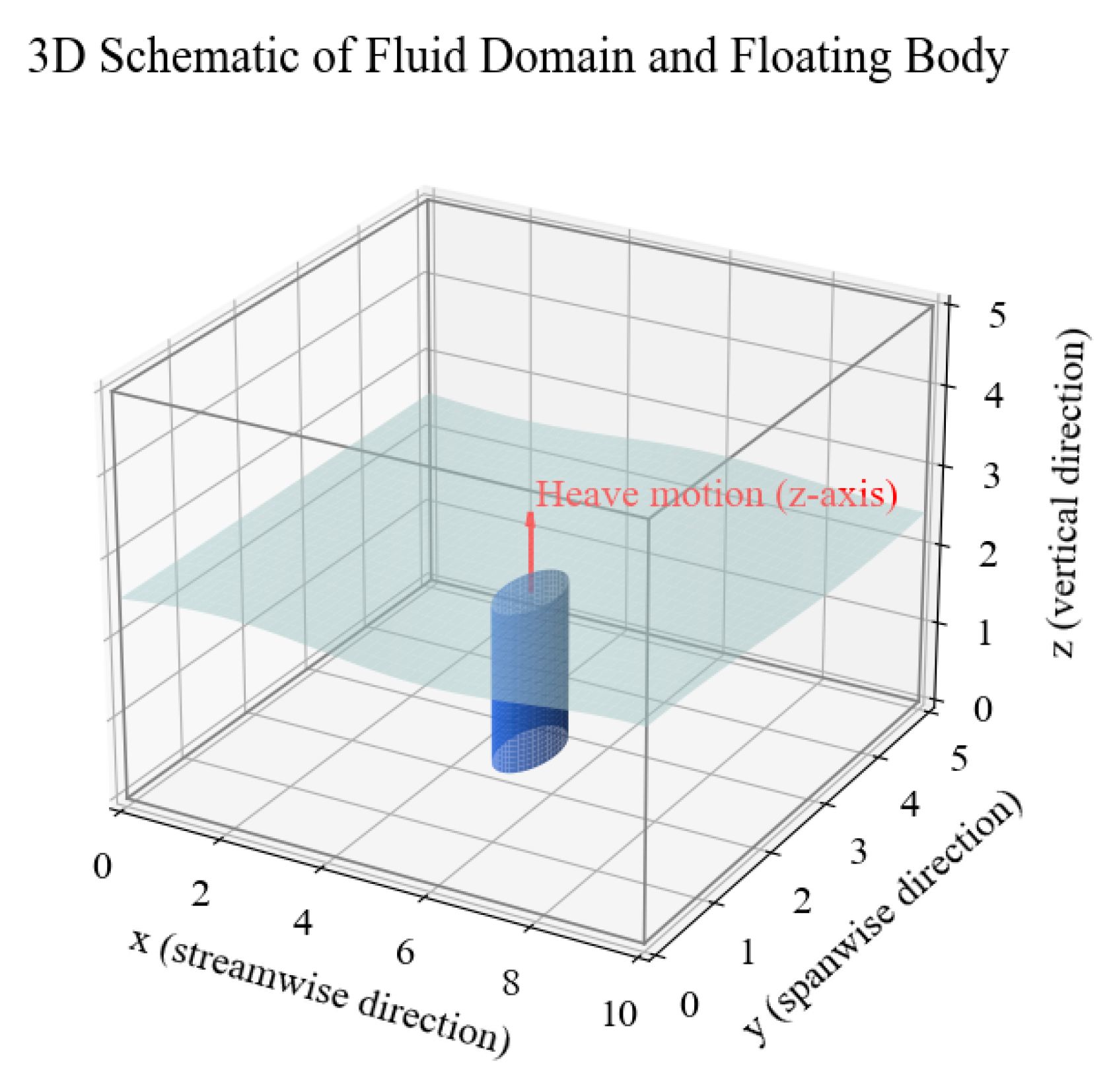
Figure 1: Three-dimensional schematic of the computational domain and floating body with defined coordinate axes and single degree of freedom.

To systematically characterize the vortex-induced vibration characteristics under different flow velocities and incident angles, the simulation conditions are designed concerning the marine environmental load classification scheme for typical semi-submersible floating structures in the DNV-RP-C205 and API RP 2A standards, and the common working condition combinations in typical representative wind, wave, and current combined action scenarios are selected, from which 5 groups of typical working conditions are extracted for simulation. The total number of working conditions in actual engineering applications far exceeds the number selected in this simulation; however, the following parameters cover the common operating environment and extreme environment range, and their settings are shown in Table 3.

According to the simulation calculation results, a significant periodic vortex shedding phenomenon occurs in the wake vortex area of the floating structure, and the vortex street frequency and the lateral vibration response of the structure form a locking area. Its spatiotemporal evolution process is shown in Fig. 2, which demonstrates the formation mechanism of the periodic response of the structure under high Reynolds number conditions and provides a temporal flow characteristic basis for the subsequent input construction of the neural network model.

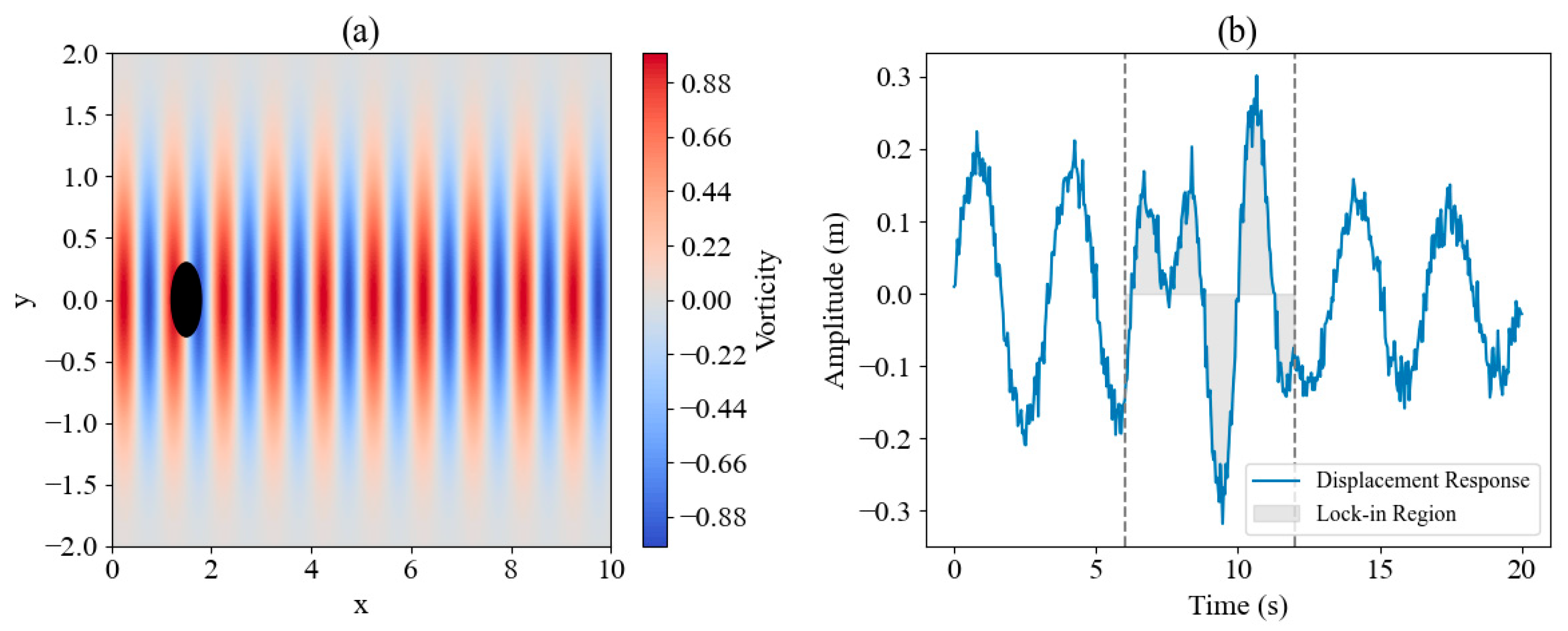
Figure 2: Schematic diagram of transient vortex-induced response in non-structural CFD simulation. (a): Vorticity field distribution; (b): Structural displacement response.

Fig. 2 shows the fluid-structure interaction response characteristics under typical vortex-induced vibration conditions. The left side shows the instantaneous vorticity distribution near the wake region, highlighting the alternating shedding of coherent vortices downstream of the structure. This flow pattern represents the initiation of the periodic wake formation process rather than a fully developed Kármán vortex street. The right side displays the corresponding displacement response curve, in which the middle section identifies a quasi-steady amplitude region where the response frequency remains synchronized with the dominant vortex shedding frequency, denoting a frequency-locking interval caused by vortex–structure resonance.

After completing the CFD simulation, the time series features such as the flow field pressure distribution P x , y , z , t , the velocity vector field U i x , y , z , t , i = 1 , 2 , 3 , and the structural response displacement x t are extracted to construct a three-dimensional input tensor X ∈ ℝ T × C × L , where T represents the number of time steps, C represents the number of input channels (pressure, velocity components and structural response), and L represents the number of discrete nodes in the structural space. The displacement x t obtained from the structural response is a scalar quantity representing the heave motion amplitude at each time step. To maintain dimensional consistency across the input tensor, this scalar value is spatially broadcast across all corresponding [x, y, z] nodes of the fluid field at the same time instant. This ensures that each tensor frame contains synchronized information on local flow quantities and the global structural motion, allowing the convolutional layers to learn the spatial correlation between flow fluctuation and displacement evolution. The tensor is normalized and used as the input of the deep neural network model, where each channel value is uniformly mapped to the interval [0, 1], and the normalization method is:

Each sample contains 100 consecutive frames of transient response data, and the prediction target is the peak amplitude and main frequency value at the end of the corresponding time window. To ensure that the input of model training maintains high information density, the effective frame interval of CFD output is screened by spectral entropy analysis to eliminate the initial stage of stable flow state and the unresponsive disturbance section. Through high-resolution modeling of unstructured grids and extraction of multi-dimensional physical feature tensors of CFD simulation data, the input construction process required for vortex-induced vibration response prediction is completed, providing an input basis with spatial coupling and temporal dynamics for the subsequent attention convolutional network model, and effectively retaining the key information distribution of structure-flow field interaction.

It should be noted that the role of CFD in this study is confined to the generation of high-fidelity physical data for network training and validation. Once the SE-CNN model is trained, it serves as a surrogate model that directly predicts the vibration amplitude and dominant frequency for new flow conditions without rerunning CFD simulations. This substitution eliminates the repeated cost of numerical computation, as the trained network performs inference within milliseconds for each new input tensor. Consequently, the proposed hybrid approach achieves substantial computational efficiency while preserving the physical interpretability provided by CFD-derived data.

3.2 SE-CNN Structure Design and Attention Mechanism Integration

This section elaborates on the structural implementation process of the constructed SE-CNN and its mechanism of action in the prediction task of vortex-induced vibration response of floating structures. The network uses a multi-layer convolutional structure to extract the spatial and temporal features of the input three-dimensional time series feature tensor, and embeds a channel attention module at each stage to strengthen the weight expression of key response features, thereby improving the model’s ability to recognize the nonlinear relationship between high-frequency disturbances and low-frequency ground state responses.

The input tensor is set to the three-dimensional feature tensor X ∈ ℝ T × H × W × C , where T represents the number of time frames, H and W are the two-dimensional spatial dimensions of each frame, and C is the number of channels. The input channel consists of the pressure field, velocity gradient field, and structural displacement field generated by CFD simulation. The convolution operation is defined as a standard three-dimensional convolution:

In Formula (8), ∗ represents the convolution operation; W is the convolution kernel weight tensor; b is the bias term; δ is the nonlinear activation function ReLU. The above convolution layer configuration uses a 3 × 3 × 3 convolution kernel, a step size of 1, and a padding strategy of the same size to maintain the spatial dimension unchanged.

The SE module is applied after the output of the convolutional layer to adaptively redistribute the importance weights of each channel. The SE module first performs global average pooling on the channel dimension to obtain the statistical feature vector z c of each channel:

The compressed channel description vector z ∈ ℝ C is input into the activation function structure consisting of two fully connected layers, and the attention weight of each channel is obtained through a nonlinear mapping:

In Formula (10), σ represents the ReLU activation function; δ represents the Sigmoid function; W 1 ∈ ℝ C / r × C and W 2 ∈ ℝ C × C / r are the weight matrices of the dimension reduction and dimension increase operations, respectively; r is the compression scale factor, which is set to 16 to balance the model’s expressiveness and parameter scale. Finally, the feature map of each channel is scaled channel by channel according to the weight s to enhance the key response channel:

The SE module is inserted after each group of convolutional modules to achieve hierarchical enhancement of multi-scale response information. Fig. 3 illustrates the overall network structure of SE-CNN, highlighting the insertion path and action area of the SE module in each convolutional layer.

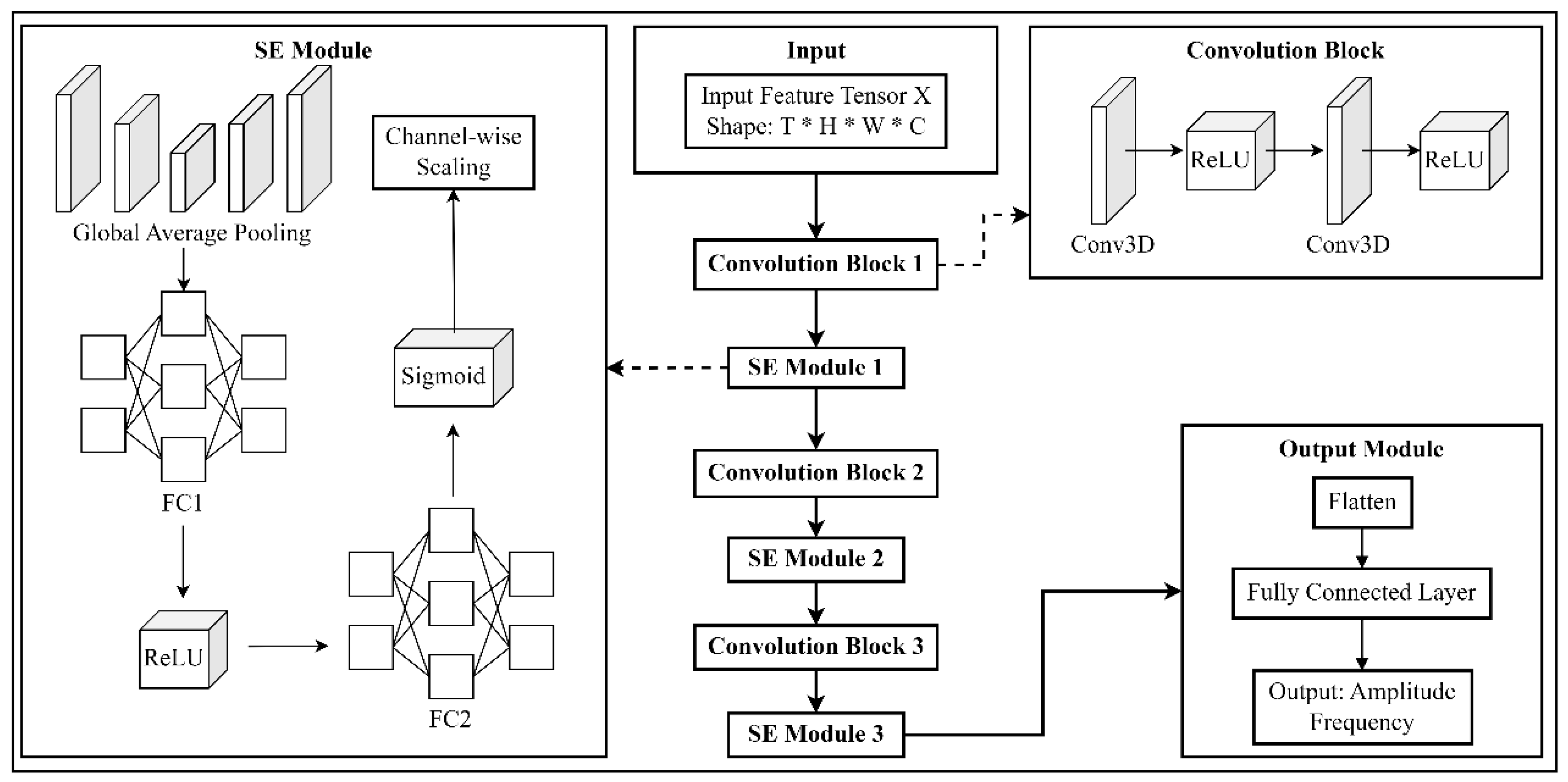
Figure 3: Schematic diagram of SE-CNN network structure.

The network consists of three convolutional blocks (each block contains two convolutional layers), and each convolutional block is embedded with a set of SE modules. After the extraction is complete, the response prediction regression is performed using a fully connected layer. The model structure uses Mean Squared Error (MSE) as the loss function, which is defined as:

In Formula (12), y i and y ^ i are the true value and predicted value of the i -th sample, respectively, and N is the number of samples.

To verify the enhancement effect of the attention mechanism on the intermediate features of the model, Table 4 lists the comparison results of SE-CNN and ordinary CNN under the entropy index of the feature map output of the intermediate convolution layer. The feature map entropy is used to measure the quality of the distribution of channel information extracted by the model. The larger the entropy value, the more dispersed the information and the weaker the channel recognition. The lower the entropy value, the more concentrated the channel recognition and the more effective the attention enhancement.

The results in Table 4 show that after the application of the SE module, the entropy of the output feature map of each layer has decreased significantly, indicating that the model effectively focuses on a few key response channels, improves the ability to identify structural vibration response characteristics, and enhances the response accuracy to high-frequency disturbance information. The overall network structure and attention path design significantly optimize the response mapping relationship between multi-dimensional input features through structural reinforcement and channel reconstruction, providing stable and accurate feature extraction support for subsequent vortex-induced vibration prediction tasks.

3.3 Model Training and Prediction Process Description

The model training phase utilizes the constructed three-dimensional time series feature tensor as input, mapping the output to the vortex-induced vibration response value of the floating structure within the corresponding time window, which includes the lateral amplitude and the main vibration frequency [38]. The input tensor is in the form of X ∈ ℝ T × H × W × C , where T represents the number of time frames, H × W is the spatial dimension of the feature map, and C is the number of channels, corresponding to the three physical quantities of pressure field, velocity gradient field, and structural response field. The network output is y ∈ ℝ 2 , which corresponds to the maximum response amplitude A m a x and the main vibration frequency f d o m in the time window.

The training process uses the Adam optimizer, and the loss function is designed as a weighted regression loss to jointly minimize the amplitude error and frequency deviation. Defining the predicted output as A ^ m a x , f ^ d o m and the actual value as A m a x , f d o m , then the total loss function L t o t a l is expressed as:

In Formula (13), α and β are loss weight hyperparameters, and the MSE L A of the amplitude is calculated by Formula (14):

The MSE L f of frequency is calculated by Formula (15):

The values are set to α = 0.6 and β = 0.4 after cross-validation. The training data is divided into a 70% training set, a 15% validation set, and a 15% test set to maintain consistency across various working conditions within the data subsets, thereby avoiding sample bias that can cause model overfitting.

The input data is standardized in the preprocessing stage to a zero mean unit variance form, and the normalization operation is defined as:

In Formula (16), x represents the single-point value of the original data tensor, and μ x and σ x are the mean and standard deviation of all samples of the channel, respectively. The normalization operation maintains the stability of the gradient propagation of each input channel in the network and improves the efficiency of model training.

The neural network training employs the batch gradient descent strategy, with a batch size of 64, 200 total training rounds, and an initial learning rate of 10−3. The learning rate is dynamically adjusted by a factor of 0.5 when the validation set loss does not decrease. To improve the training stability, the L2 regularization term is applied to suppress model overfitting, and its expression is:

In Formula (17), L represents the total number of network layers; W l is the weight tensor of the convolution kernel of the l -th layer; λ is the regularization coefficient, which is set to 10−4. The final training goal is to minimize the total loss in the following formula:

After each round of training, the model is evaluated on the validation set, and the Mean Relative Error (MRE) is calculated. The expression of MRE is:

The frequency prediction deviation is defined as the absolute difference Δ f = f ^ d o m − f d o m , which is an important indicator for evaluating the accuracy of high-frequency disturbance recognition. During the training process, the loss value and error index change curve of each round are recorded to analyze the model convergence speed and training stability.

During the test phase, the three-dimensional tensor sequence in the test set is input, and the model outputs the corresponding response value. The overall error and deviation distribution are then statistically analyzed. Under the premise of ensuring the consistency of the input scale, all predicted values are denormalized physical quantities to ensure the engineering interpretability of the results and the feasibility of subsequent visual analysis. The model prediction results are used as data support for the subsequent response control strategy formulation and fatigue life assessment module.

4 Experimental Design and Configuration

4.1 Dataset Construction and Annotation Instructions

This section constructs a dataset of floating structure vortex-induced vibration responses based on the unstructured grid CFD simulation results. The simulation encompasses various flow velocities, incident angles, and structural damping conditions to determine the flow field and structural dynamic response under typical working conditions. All data samples are derived from CFD numerical simulations, based on a typical semi-submersible floating body model, combined with the DNV-RP-C205 and API RP 2A environmental specifications to ensure that the data has engineering representativeness and physical consistency. This paper adopts a local encrypted unstructured grid division strategy to obtain high-resolution pressure field, velocity gradient field, and structural displacement sequence. All output data are uniformly time-series aligned and standardized to form a three-dimensional feature tensor as neural network input. The response annotation targets are the maximum displacement and main vibration frequency of the structure, which reflect the amplitude change trend and spectrum characteristics, respectively, and are annotated using steady-state segment extraction and frequency domain analysis methods.

To study the coverage and response characteristics of the sample library in the dimensions of the main physical parameters, the statistical distribution of the VIV data set under typical simulation conditions is given in Table 5, including flow velocity, incident angle, damping ratio, number of grids, maximum displacement and main frequency range, and number of samples. The data is derived from CFD simulation results under various boundary condition configurations, ensuring that all response modes are fully represented in the training set.

As can be seen from Table 5, the data set covers the low, medium, and high speed vortex-induced vibration flow field characteristic intervals commonly seen in marine engineering. The structural damping ratio setting covers typical engineering requirements. The maximum displacement and main frequency show an obvious segmentation trend in each group. The number of grids increases with the increase of flow velocity, reflecting the simulation’s need to capture local vortex structures in scenarios of different complexity. The number of samples remains relatively balanced between groups, effectively supporting the generalization modeling capabilities of neural networks under a variety of input conditions. The construction method and annotation standards of the data set ensure that subsequent model training has sufficient stability, representativeness, and consistency with prediction targets.

4.2 Experimental Environment and Training Parameter Settings

The neural network model constructed in this section employs a multi-channel convolutional residual structure to efficiently extract and map the response of the flow field time series features, which are input in the form of three-dimensional tensors. The overall structure consists of an input module, a local perception module, a global perception module, and an output mapping module. The core is to apply a multi-scale convolution kernel combination and a cross-channel attention mechanism to collaboratively model local disturbances and global flow trends. The input layer accepts a standardized three-dimensional tensor, which contains three physical quantity dimensions: pressure field, velocity gradient field, and structural boundary surface displacement, and is expanded on the time axis to form a frame sequence. The local perception module consists of two 3 × 3 × 3 convolution blocks, utilizing ReLU and BatchNorm for nonlinear enhancement and feature normalization. The global perception module uses a hole convolution and residual connection superposition method to expand the receptive field while suppressing the risk of gradient vanishing. The output mapping module includes a two-layer fully connected structure, which is used to map the fused deep semantic features to two scalar outputs: maximum displacement and main frequency.

To ensure the stability and generalization ability of model training, all convolutional layers are initialized using the He method. The optimizer is Adam; the loss function is weighted MSE; the maximum displacement prediction deviation is penalized. The Dropout ratio is set to 0.2 to control overfitting. The batch size is 32; the upper limit of the training round is set to 300; the Early Stop strategy is used to prevent invalid iterations. Table 6 lists the specific configuration parameters of each module.

The network structure fully integrates temporal dynamics and spatial disturbance information while ensuring a balance between depth and width. The channel attention mechanism effectively enhances the expression coupling between feature dimensions, and the dilated convolution expands the ability to model the impact of far-field vortices on structural responses. The parameter configuration has been verified through multiple rounds of ablation experiments, and the current structure shows better convergence speed and prediction accuracy on the validation set.

5 Result Analysis

5.1 Comparative Analysis of Amplitude Prediction Accuracy

To evaluate the prediction accuracy of the SE-CNN model for the amplitude response of floating structures under various typical working conditions, this paper designs a comparative experiment for five groups of representative incoming flow velocity ranges. The experiment obtains the real vibration response sequence through unstructured grid CFD simulation, corresponding to the velocity ranges of 0.4–0.8 m/s, 0.8–1.2 m/s, 1.2–1.4 m/s, 1.4–1.6 m/s and 1.6–1.8 m/s, and uses the trained SE-CNN model for parallel prediction, records the real and predicted amplitude curves, and calculates the relative error index under each working condition, to realize the visual analysis of the vibration response prediction ability under multi-speed conditions. The relevant results are shown in Fig. 4.

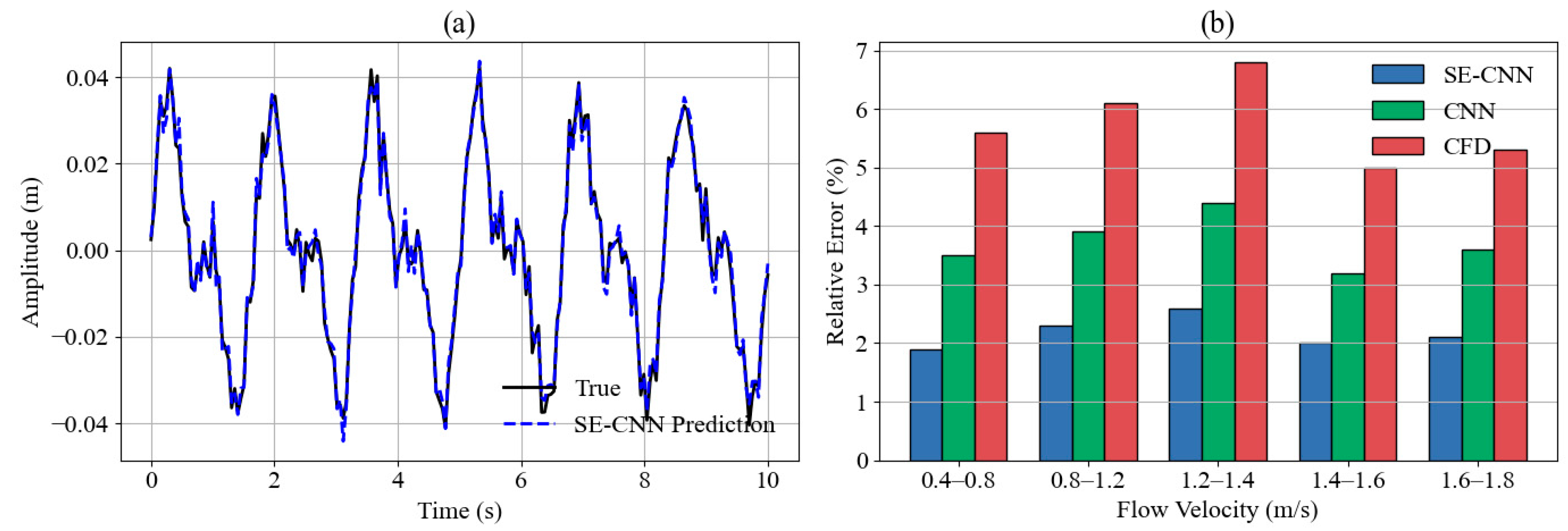
Figure 4: Comparison of amplitude response prediction results. (a): Actual and predicted amplitude response curves under typical working conditions; (b): Relative error of amplitude prediction under different flow rate ranges.

The SE-CNN prediction curve in Fig. 4a is highly consistent with the actual vibration response, and the amplitude change is consistent with the periodic trend as a whole, with only slight offsets at some peaks and valleys. The model has a strong fitting ability in modeling the dynamic evolution law of structural response. The main reason for the stable prediction accuracy is that the channel attention mechanism enhances the model’s selective response to key components of the flow disturbance, allowing it to extract the primary modal features while suppressing non-target noise interference. Fig. 4b shows that SE-CNN has the lowest error in the range of 0.4–0.8 m/s, achieving an error rate of 1.9%. Within this range, the flow pattern is relatively regular, and the structural response frequency remains stable, which is conducive to model convergence. The error is as high as 2.6% in the range of 1.2–1.4 m/s. In this range, the vortex excitation frequency is close to the natural frequency of the structure, inducing a strong resonance effect that enhances vibration amplitude fluctuations and disturbs the model’s channel weight distribution, resulting in a decrease in output accuracy. In comparison, CNN and CFD exhibit higher errors in all intervals, with the lowest error of CNN reaching 3.2%, indicating obvious frequency drift and amplitude deviation, primarily due to their limited ability to distinguish local disturbance components. The analysis results show that SE-CNN has higher adaptability and robustness in multi-scale response modeling tasks under different flow velocity fields.

5.2 Evaluation of the Control Capability of Main Frequency Prediction Error

To evaluate the error control ability of different methods in the main frequency prediction task, a typical flow velocity segment is selected to construct a frequency domain test set, and the performance of SE-CNN, CNN, and traditional CFD methods in terms of main frequency prediction accuracy is compared. In the experiment, the inherent main frequency of the structure is set to 1.20 Hz as a reference standard for evaluating the accuracy of each method’s output. Each method outputs the corresponding predicted main frequency in five flow velocity intervals, and the frequency error distribution is obtained by calculating the difference between it and the true value, which further characterizes the robustness and accuracy retention ability of different methods under changing flow velocities. The corresponding error results are shown in Fig. 5.

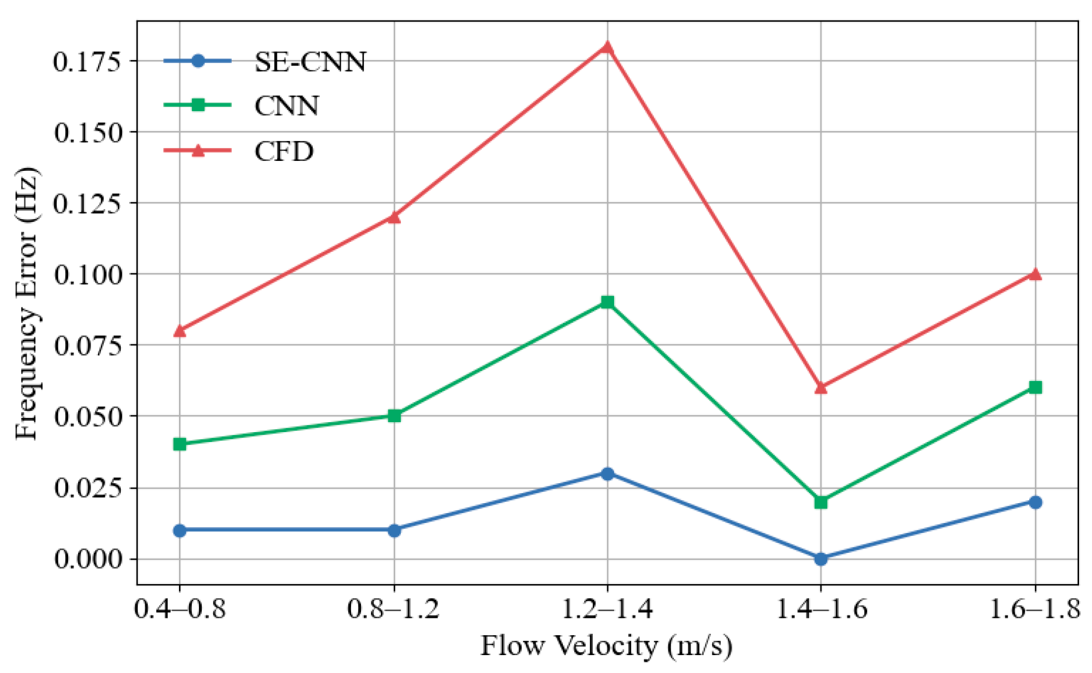
Figure 5: Comparison of main frequency prediction deviation.

Fig. 5 shows that in the flow velocity range of 1.2–1.4 m/s, the frequency prediction error of the CFD method is 0.18 Hz, which is significantly higher than those of CNN (0.09 Hz) and SE-CNN (0.03 Hz). The primary reason is that the CFD solution lacks a noise suppression mechanism for frequency extraction in the transient response, resulting in a shift in the positioning of the main spectral peak. Although CNN alleviates some fluctuations through end-to-end learning, it is still limited by the insufficient frequency density of training samples in this range, and the deviation is aggravated. In contrast, SE-CNN achieves zero error in the flow velocity range of 1.4–1.6 m/s, primarily due to its enhanced modeling ability of the residual signal structure in the low-frequency band, which improves the stability and accuracy of spectrum extraction. Across the entire range, the frequency error of the SE-CNN method is consistently controlled within 0.03 Hz, demonstrating strong consistency in frequency domain fitting and anti-interference ability.

5.3 Visualization of Feature Channel Weight Distribution and Model Attention Area

In the process of modeling the channel attention mechanism, to explore the distribution changes of the response characteristics of different depth convolutional layers to the input physical quantity, this study constructs the channel average activation heat map of the three network node positions of the shallow, middle and deep layers, extracts the feature maps of the corresponding convolution output, and calculates the average activation value after normalizing the response intensity of each channel to form a 9-channel matrix input thermal analysis module. Considering the sensitivity of the SE module to the channel-weighted allocation, this process enables the observation of the selective enhancement trend of the network across different channel dimensions as it evolves with depth, thereby revealing its preference distribution for different input types during the feature extraction stage, as shown in Fig. 6.

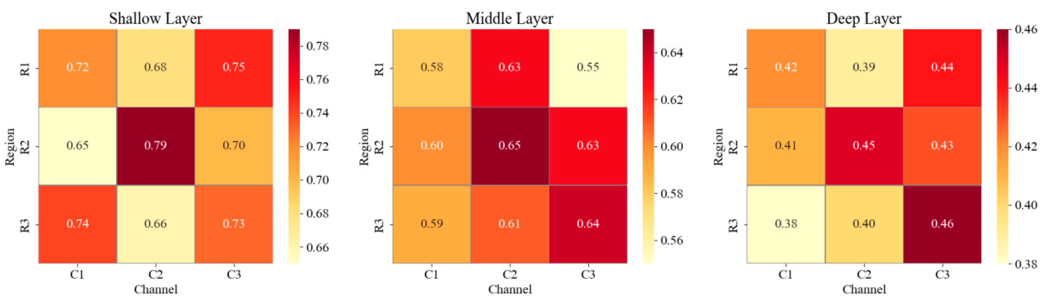
Figure 6: Heat map of channel response strength of different convolutional layers.

In Fig. 6, the overall activation level of the shallow convolution feature map is maintained in a high range, with an average response value between 0.65 and 0.79, among which the C2 channel reaches a maximum value of 0.79 at the R2 position, indicating that the activation level of all input physical fields is generally strong in the early stage of the network. This is mainly because the shallow convolution weights have not yet formed a significant difference distribution, and the primary features of the structural displacement and velocity gradient are widely captured. After entering the middle layer, the response intensity is significantly weakened, and the activation value decreases to a range of 0.55 to 0.65 overall. Among them, the C2 channel maintains a relatively dominant position, with an average value of 0.63. This trend of feature concentration is related to the SE module’s increasing emphasis on the dominant channel response, and the distinction between physical inputs gradually deepens as the level advances. In deep convolution, the channel activation value further shrinks to the range of 0.38 to 0.46, and the C3 channel maintains the highest response of 0.46 at the R3 position. The activation distribution of other channels tends to be sparse. This phenomenon is caused by the high abstractness of deep convolution features, which only respond to a small number of key physical variables. It is the result of the network compressing redundant inputs and strengthening dominant features. The overall trend indicates that the attention of network channels exhibits selective convergence as the level of depth increases.

The experiment selects the channel weight coefficient of the middle layer in SE-CNN as the key indicator. It extracts the model’s attention weight distribution for different input channels at continuous time steps, thereby analyzing the channel attention behavior of the attention convolution model during the processing of multimodal physical input. By setting an input window containing 20 time steps, the weight evolution trend of the three physical channels—Pressure, Velocity Gradient, and Displacement—in the time dimension is tracked, and then the dynamic adjustment strategy of the model to the response characteristics of various input physical quantities is revealed. The relevant results are shown in Fig. 7. Pressure represents the instantaneous pressure distribution in the flow field; Velocity Gradient reflects the spatial change rate of the local velocity field; Displacement represents the response displacement of the structure under vortex excitation.

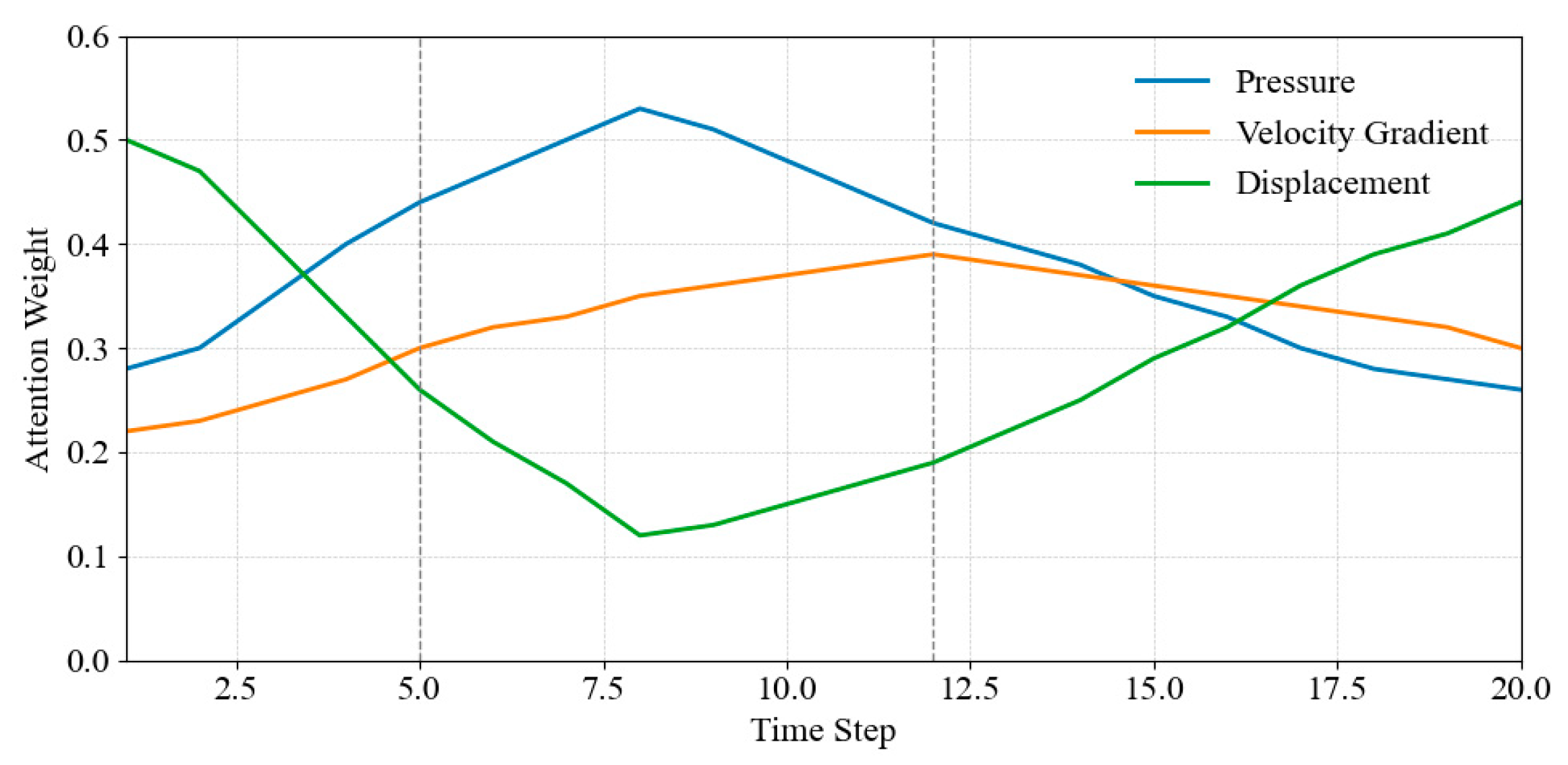
Figure 7: Weighted trend of attention channel evolution over time.

Fig. 7 shows that, in the first 8 time steps, the attention weight of the Pressure channel gradually increases from 0.28 to 0.53 and reaches a peak at the 8th step, indicating that the model pays more attention to the pressure change during the rising stage of the flow field disturbance. This trend is closely related to the significant fluctuations in the pressure gradient during the early stage of vortex structure formation. The weight of the Displacement channel decreases from 0.50 to 0.12 in the early stage and then gradually increases, reaching 0.44 by the 20th step. This distribution pattern of first depression and then rise is due to the significant enhancement of the structural displacement response in the later stage of vortex excitation, which guides the model to refocus on this channel. The channel weight of Velocity Gradient is at a medium level overall, with a fluctuation range of 0.22 to 0.39, indicating that it maintains a stable contribution throughout the process but does not significantly influence the model decision. The weighted changes in the SE mechanism on the physical channel reflect the response and adjustment capabilities of the stage characteristics in fluid-solid evolution, thereby improving the model’s time series identification accuracy of input information.

5.4 Verification of Multi-Condition Adaptability and Generalization Ability

The experiment establishes experimental conditions encompassing six typical structural damping ratios. It obtains corresponding vibration response data, based on a unified flow velocity and flow direction input configuration, to evaluate the model’s response prediction robustness under varying damping conditions. The prediction results of the SE-CNN model and the conventional CNN model, without the attention mechanism, are statistically analyzed at each damping ratio, with MRE used as the evaluation index. The response consistency and error concentration of the model under each condition are analyzed through distribution patterns. The results are presented in Fig. 8, which illustrates the distribution characteristics of the prediction error for the two types of models in multi-damping scenarios.

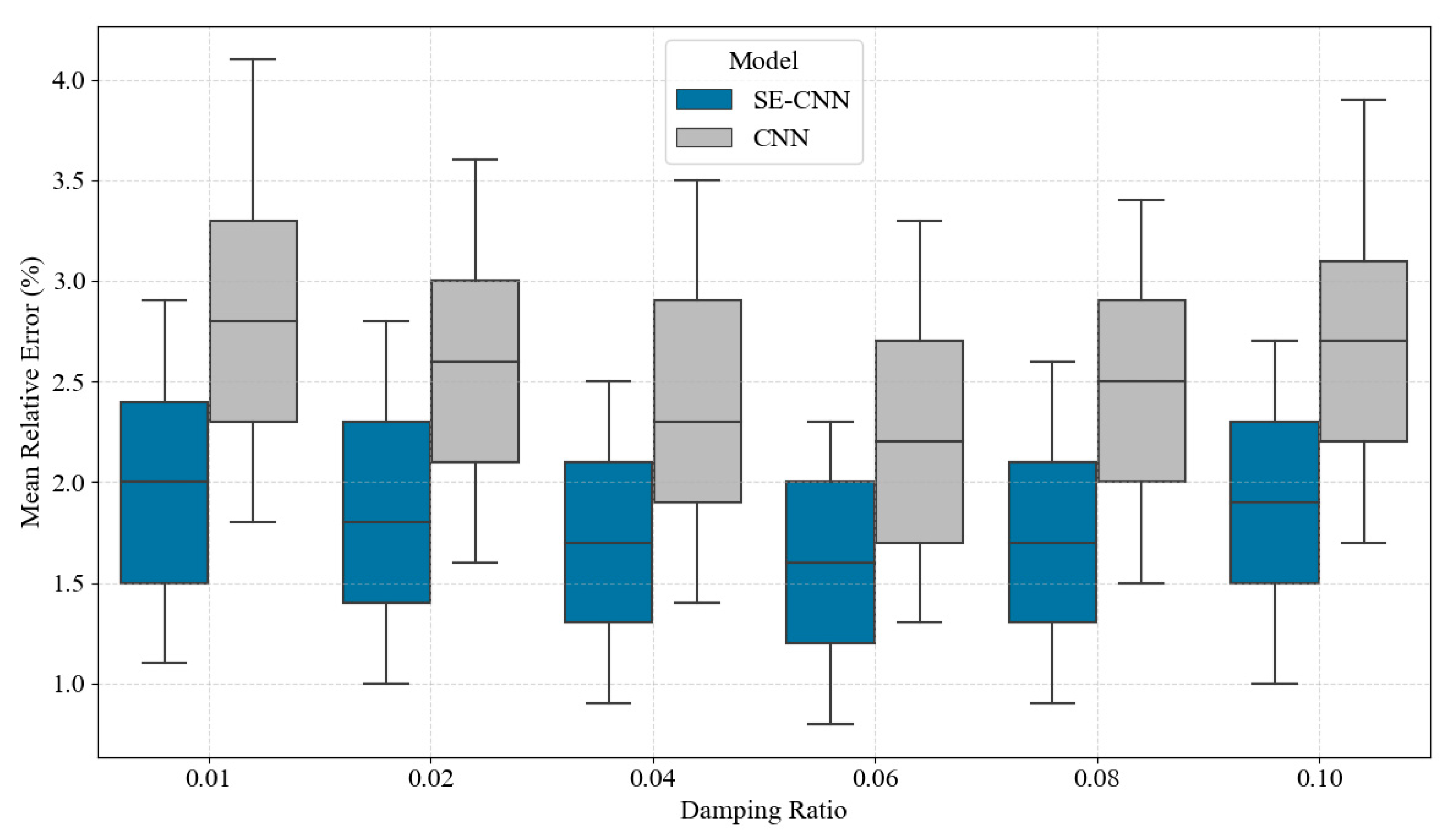
Figure 8: Comparison of prediction error distribution under different damping ratios.

Fig. 8 shows that under the condition of a low damping ratio of 0.01, the median prediction error of the SE-CNN model is 2.0%, and the maximum error does not exceed 2.9%. In comparison, the median error of the ordinary CNN under the same conditions reaches 2.8%, and the upper limit of the error is expanded to 4.1%. This difference is primarily influenced by the channel enhancement effect of the SE module on the high-frequency perturbation response, which enables it to better extract small vibrations under low energy consumption. When the damping ratio increases to 0.06, the error range of SE-CNN is further tightened, with a median of 1.6% and a maximum value of 2.3%. In contrast, the maximum error of the ordinary CNN under this damping reaches 3.3%. This trend indicates that the attention mechanism exhibits stronger selective sensitivity to the area where the response signal energy is concentrated, thereby suppressing the influence of non-main modes on the output error and ultimately demonstrating higher prediction consistency and error control ability under various damping conditions.

5.5 Comparison of Model Convergence and Training Efficiency

During the training process, to comprehensively evaluate the learning ability and efficiency performance of the model, this experiment compares SE-CNN, the standard CNN structure, and the simplified model (No Attention) after removing the attention module, focusing on the differences in the training error convergence speed and the growth trend of training time. In the model convergence experiment, the loss function value of each round of training is used as the basis for horizontal comparison; in the training efficiency test, the total time accumulated in different rounds of training is recorded, and the same hardware environment and optimizer configuration are used to ensure the fairness of the comparison. The experimental results are presented in Fig. 9, which illustrates the changes in Loss with Epoch during the training process of each model, along with the corresponding cumulative training time.

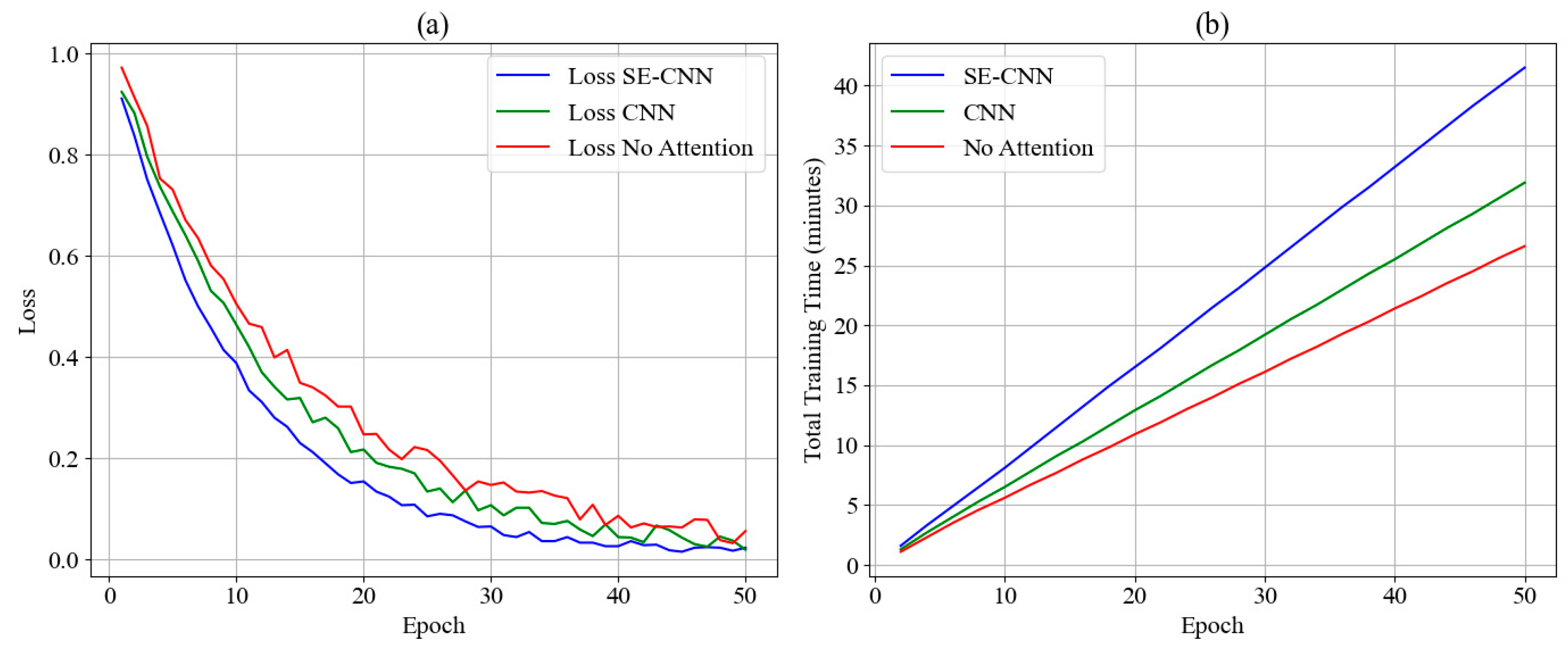
Figure 9: Comparison of model training process. (a): Loss convergence curves of different models; (b): Training time growth trend of different models.

Throughout the entire training process, from the 1st round to the 50th round, the loss value of the SE-CNN model decreases from 0.911 to 0.023, resulting in an overall decrease of 0.888, exhibiting a stable and rapid convergence trend. In contrast, the Loss of the CNN model drops from 0.924 to 0.019. Although the final value is slightly lower, the fluctuation range is large during the decline, and the platform experiences multiple stages. The No Attention model drops from 0.972 to 0.056, and the overall convergence curve is relatively gentle. The fundamental reason for this performance gap is that the SE module effectively enhances the correlation modeling ability between feature channels, improves the expression efficiency of high-dimensional semantic features through the weight recalibration mechanism, and thus accelerates the compression process of model errors. In terms of training time, the cumulative training time of SE-CNN in 50 rounds is 41.5 min, which is significantly higher than the 31.9 min of the CNN model and the 26.6 min of the No Attention model. Its main cost comes from the calculation delay caused by the compression and activation operations applied by channel attention. Overall, SE-CNN has more advantages in terms of convergence performance; however, the increase in computing cost requires weighing the deployment strategy according to the specific application scenario.

6 Conclusion

The unstructured grid CFD and SE-CNN fusion modeling method proposed in this paper obtains the high-dimensional time series feature tensor of multi-physical field coupling through the finite volume method, constructs a multi-channel input structure, takes pressure, velocity gradient, and structural response as input, applies the channel attention mechanism in the convolution stage to strengthen the expression of key response areas, and improves the accuracy of vortex-induced vibration modeling. The experimental results show that the relative error of amplitude prediction in the flow velocity range of 0.4–0.8 m/s is 1.9%, and the main frequency prediction error in the range of 1.2–1.4 m/s is as low as 0.03 Hz. The entropy value of the third-layer feature map of the model is reduced by 0.58 compared with the traditional CNN, reflecting the improvement of channel recognition ability and the effective enhancement of key disturbance characteristics by the attention mechanism. This method significantly enhances the model’s ability to characterize nonlinear responses under complex flow conditions. While improving the accuracy of structural vibration prediction, it has high adaptability to multiple working conditions and training convergence efficiency, providing stable and efficient technical support for the safety assessment and design optimization of floating structures in complex marine environments.

References

1. Fujarra ALC , Cenci F , Silva LSP , Hirabayashi S , Suzuki H , Gonçalves RT . Effect of initial roll or pitch angles on the vortex-induced motions (VIM) of floating circular cylinders with a low aspect ratio. Ocean Eng. 2022; 257: 111574. doi:10.1016/j.oceaneng.2022.111574. [Google Scholar] [CrossRef]
2. Naqash TM , Alam MM , Naqash TM , Alam MM . A state-of-the-art review of wind turbine blades: principles, flow-induced vibrations, failure, maintenance, and vibration suppression techniques. Energies. 2025; 18( 13): 3319. doi:10.3390/en18133319. [Google Scholar] [CrossRef]
3. Alkarem YR , Ozbahceci BO . A complemental analysis of wave irregularity effect on the hydrodynamic responses of offshore wind turbines with the semi-submersible platform. Appl Ocean Res. 2021; 113: 102757. doi:10.1016/j.apor.2021.102757. [Google Scholar] [CrossRef]
4. Ijaz A , Manzoor S . Vortex induced vibration prediction through machine learning techniques. AIP Adv. 2024; 14( 11): 115025. doi:10.1063/5.0236511. [Google Scholar] [CrossRef]
5. Habibnia Rami M , Carlos Pascoa J . Coupled active control technique for oscillating blades in a cycloidal rotor using CFD and ANN analysis by including 3D end wall effects. J Aerosp Eng. 2021; 34( 6): 04021089. doi:10.1061/(asce)as.1943-5525.0001332. [Google Scholar] [CrossRef]
6. Malliotakis G , Alevras P , Baniotopoulos C . Recent advances in vibration control methods for wind turbine towers. Energies. 2021; 14( 22): 7536. doi:10.3390/en14227536. [Google Scholar] [CrossRef]
7. Amaechi CV , Reda A , Butler HO , Ja’e IA , An C . Review on fixed and floating offshore structures. Part I: types of platforms with some applications. J Mar Sci Eng. 2022; 10( 8): 1074. doi:10.3390/jmse10081074. [Google Scholar] [CrossRef]
8. Ahmad Azlan NH , Shaharuddin NMR , Ali A . Influence of connector forces on the expansion configuration of a hexagonal modular floating structure. Chall J Struct Mech. 2025; 11( 2): 89. doi:10.20528/cjsmec.2025.02.003. [Google Scholar] [CrossRef]
9. Bai XD , Zhang W . Machine learning for vortex induced vibration in turbulent flow. Comput Fluids. 2022; 235: 105266. doi:10.1016/j.compfluid.2021.105266. [Google Scholar] [CrossRef]
10. Misaka T . Estimation of vortex-induced vibration based on observed wakes using computational fluid dynamics-trained deep neural network. J Fluids Eng. 2021; 143( 10): 104501. doi:10.1115/1.4050974. [Google Scholar] [CrossRef]
11. Yan Z , Zheng S , Yang F , Tai X , Chen Z . A simplified approach to recognize vortex-induced vibration response using machine learning. Struct Eng Int. 2024; 34( 4): 670– 82. doi:10.1080/10168664.2023.2287460. [Google Scholar] [CrossRef]
12. Schubert Y , Sieber M , Oberleithner K , Martinuzzi R . Towards robust data-driven reduced-order modelling for turbulent flows: application to vortex-induced vibrations. Theor Comput Fluid Dyn. 2022; 36( 3): 517– 43. doi:10.1007/s00162-022-00609-y. [Google Scholar] [CrossRef]
13. Rahimilarki R , Gao Z , Jin N , Zhang A . Convolutional neural network fault classification based on time-series analysis for benchmark wind turbine machine. Renew Energy. 2022; 185: 916– 31. doi:10.1016/j.renene.2021.12.056. [Google Scholar] [CrossRef]
14. Liu T , Huang Z , Tian L , Zhu Y , Wang H , Feng S . Enhancing wind turbine power forecast via convolutional neural network. Electronics. 2021; 10( 3): 261. doi:10.3390/electronics10030261. [Google Scholar] [CrossRef]
15. Stone E , Giani S , Zappalá D , Crabtree C . Convolutional neural network framework for wind turbine electromechanical fault detection. Wind Energy. 2023; 26( 10): 1082– 97. doi:10.1002/we.2857. [Google Scholar] [CrossRef]
16. Choe DE , Kim HC , Kim MH . Sequence-based modeling of deep learning with LSTM and GRU networks for structural damage detection of floating offshore wind turbine blades. Renew Energy. 2021; 174: 218– 35. doi:10.1016/j.renene.2021.04.025. [Google Scholar] [CrossRef]
17. Li Z , Luo X , Liu M , Cao X , Du S , Sun H . Short-term prediction of the power of a new wind turbine based on IAO-LSTM. Energy Rep. 2022; 8: 9025– 37. doi:10.1016/j.egyr.2022.07.030. [Google Scholar] [CrossRef]
18. Zhang F , Zhu Y , Zhang C , Yu P , Li Q . Abnormality detection method for wind turbine bearings based on CNN-LSTM. Energies. 2023; 16( 7): 3291. doi:10.3390/en16073291. [Google Scholar] [CrossRef]
19. Qin S , Tao J , Zhao Z . Fault diagnosis of wind turbine pitch system based on LSTM with multi-channel attention mechanism. Energy Rep. 2023; 10: 4087– 96. doi:10.1016/j.egyr.2023.10.076. [Google Scholar] [CrossRef]
20. Wang A , Pei Y , Zhu Y , Qian Z . Wind turbine fault detection and identification through self-attention-based mechanism embedded with a multivariable query pattern. Renew Energy. 2023; 211: 918– 37. doi:10.1016/j.renene.2023.05.003. [Google Scholar] [CrossRef]
21. Fu X , Fu S , Niu Z , Zhao B , Shen J , Deng P . A validated fluid-structure interaction simulation model for vortex-induced vibration of a flexible pipe in steady flow. Mar Struct. 2025; 104: 103895. doi:10.1016/j.marstruc.2025.103895. [Google Scholar] [CrossRef]
22. Bao J , Chen ZS . Vortex-induced vibration characteristics of multi-mode and spanwise waveform about flexible pipe subject to shear flow. Int J Nav Archit Ocean Eng. 2021; 13: 163– 77. doi:10.1016/j.ijnaoe.2021.02.003. [Google Scholar] [CrossRef]
23. Xiao ZJ , Yang SH , Yu C , Zhang Z , Sun L , Lai J , et al. Effects of cavitation on vortex-induced vibration of a flexible circular cylinder simulated by fluid-structure interaction method. J Hydrodyn. 2022; 34( 3): 499– 509. doi:10.1007/s42241-022-0038-z. [Google Scholar] [CrossRef]
24. Zou J , Zhou B , Liu H , Yi W , Lu C , Luo W . Numerical study of vortex-excited vibration of flexible cylindrical structures with surface bulge. J Mar Sci Eng. 2024; 12( 11): 1894. doi:10.3390/jmse12111894. [Google Scholar] [CrossRef]
25. Lin H , Xiang Y , Yang Y , Gao C . Fluid-vehicle-tunnel coupled vibration analysis of a submerged floating tunnel based on a wake oscillator model. J Waterway Port Coastal Ocean Eng. 2022; 148: 04021037. doi:10.1061/(asce)ww.1943-5460.0000677. [Google Scholar] [CrossRef]
26. Kharazmi E , Fan D , Wang Z , Triantafyllou MS . Inferring vortex induced vibrations of flexible cylinders using physics-informed neural networks. J Fluids Struct. 2021; 107: 103367. doi:10.1016/j.jfluidstructs.2021.103367. [Google Scholar] [CrossRef]
27. Zhu P , Liu Z , Xu Z , Lv J . An adaptive weight physics-informed neural network for vortex-induced vibration problems. Buildings. 2025; 15( 9): 1533. doi:10.3390/buildings15091533. [Google Scholar] [CrossRef]
28. Chen R , Zhang K , Luo M , An Y , Guo L . Deep learning-based prediction of pitch response for floating offshore wind turbines. J Mar Sci Eng. 2024; 12( 12): 2198. doi:10.3390/jmse12122198. [Google Scholar] [CrossRef]
29. Barooni M , Sogut DV , Barooni M , Sogut DV . Forecasting pitch response of floating offshore wind turbines with a deep learning model. Clean Technol. 2024; 6( 2): 418– 31. doi:10.3390/cleantechnol6020021. [Google Scholar] [CrossRef]
30. Roh C , Roh C . Deep-learning-based pitch controller for floating offshore wind turbine systems with compensation for delay of hydraulic actuators. Energies. 2022; 15( 9): 3136. doi:10.3390/en15093136. [Google Scholar] [CrossRef]
31. Li J , Hou G . Data-driven modeling and MPPT control of offshore wind turbines based on machine learning approach. Ocean Eng. 2025; 329: 121121. doi:10.1016/j.oceaneng.2025.121121. [Google Scholar] [CrossRef]
32. Wang H , Zhang L , Sun Y , Zou L , Wang H , Zhang L , et al. A convolutional neural network based on attention mechanism for designing vibration similarity models of converter transformers. Machines. 2023; 12( 1): 11. doi:10.3390/machines12010011. [Google Scholar] [CrossRef]
33. Alias F , Rahman MAA . A bibliometric analysis on energy harvesting from vortex-induced vibration. Cogent Eng. 2024; 11: 2386095. doi:10.1080/23311916.2024.2386095. [Google Scholar] [CrossRef]
34. Guo J , Mao R , Ma K , Chen D . Deep learning-based approach for identifying vortex-induced vibrations in stay cables. Adv Struct Eng. 2025; 28( 4): 690– 715. doi:10.1177/13694332241295594. [Google Scholar] [CrossRef]
35. Lu J , Wang Y , Zhu Y , Liu J , Xu Y , Yang H , et al. DACLnet: a dual-attention-mechanism CNN-LSTM network for the accurate prediction of nonlinear InSAR deformation. Remote Sens. 2024; 16( 13): 2474. doi:10.3390/rs16132474. [Google Scholar] [CrossRef]
36. Wang B , Cleary MJ , Masri AR . Modeling of interfacial flows based on an explicit volume diffusion concept. Phys Fluids. 2021; 33( 6): 062111. doi:10.1063/5.0053452. [Google Scholar] [CrossRef]
37. Shaheed R , Mohammadian A , Yan X , Shaheed R , Mohammadian A , Yan X . Numerical simulation of turbulent flow in bends and confluences considering free surface changes using the volume of fluid method. Water. 2022; 14( 8): 1307. doi:10.3390/w14081307. [Google Scholar] [CrossRef]
38. Bublík O , Heidler V , Pecka A , Vimmr J . Neural-network-based fluid–structure interaction applied to vortex-induced vibration. J Comput Appl Math. 2023; 428: 115170. doi:10.1016/j.cam.2023.115170. [Google Scholar] [CrossRef]
Cite This Article
Copyright © 2025 The Author(s). Published by Tech Science Press.
This work is licensed under a Creative Commons Attribution 4.0 International License , which permits unrestricted use, distribution, and reproduction in any medium, provided the original work is properly cited.
Downloads
Citation Tools