
 Submit a Paper
 Propose a Special lssue
 Open Access
ARTICLE

A Dynamic IPR Framework for Predicting Shale Oil Well Productivity in the Spontaneous Flow Stage
1 College of Petroleum Engineering, Yangtze University, Wuhan, 430100, China
2 Western Research Institute, Yangtze University, Karamay, 834000, China
3 State Key Laboratory of Low Carbon Catalysis and Carbon Dioxide Utilization, Yangtze University, Wuhan, 430100, China
* Corresponding Author: Guanglong Sheng. Email:
(This article belongs to the Special Issue: Multiphase Fluid Flow Behaviors in Oil, Gas, Water, and Solid Systems during CCUS Processes in Hydrocarbon Reservoirs)
Fluid Dynamics & Materials Processing 2025, 21(12), 3011-3031. https://doi.org/10.32604/fdmp.2025.073802
Received 25 September 2025; Accepted 11 December 2025; Issue published 31 December 2025
 View Full Text
 Download PDF
Abstract
This study investigates the unsteady flow characteristics of shale oil reservoirs during the depletion development process, with a particular focus on production behavior following fracturing and shut-in stages. Shale reservoirs exhibit distinctive production patterns that differ from traditional oil reservoirs, as their inflow performance does not conform to the classic steady-state relationship. Instead, production is governed by unsteady-state flow behavior, and the combined effects of the wellbore and choke cause the inflow performance curve to evolve dynamically over time. To address these challenges, this study introduces the concept of a “Dynamic IPR curve” and develops a dynamic production analysis method that integrates production time, continuity across multi-stage state fields, and the interactions between tubing flow and choke flow. This method provides a robust framework to characterize the attenuation trend of reservoir productivity and to accurately describe wellbore flow behavior. By applying the dynamic IPR approach, the study overcomes the limitations of conventional methods, which are unable to capture the temporal variations inherent in shale reservoir production. The proposed methodology offers a theoretical foundation for improved production forecasting, optimization of choke size, and analysis of wellbore tubing characteristics, thereby supporting more effective operational decision-making across different stages of shale reservoir development.Keywords
After undergoing fracturing and a subsequent shut-in period, shale oil production enters the depletion development stage. During this phase, the well begins to produce, relying on reservoir energy and rock elasticity. The choke, which functions as the throttling device at the wellhead, is critical; the selection of its size will directly affect the well’s production rate within a given stage and has a profound impact on the productivity and ultimate recovery factor over the entire production life cycle.
Once the reservoir enters the depletion production stage, the high-pressure field previously established in the formation, combined with the elastic energy of the rock, drives crude oil from the reservoir toward the wellbore bottom. It is then lifted to the surface through the wellbore by the action of bottomhole pressure and is ultimately produced through a surface throttling device. Therefore, the entire production process is initiated by the flow from the reservoir to the wellbore bottom. This process is typically described using the well’s Inflow Performance Relationship (IPR), which characterizes the relationship between the flow rate (Q) and the bottomhole flowing pressure (Pwf), commonly known as the IPR curve. Physically, the IPR reflects the reservoir’s fluid deliverability to the well under a given state. The study of IPRs has a long history, dating back to 1935 when Rawlins and Schellhardt established the back-pressure equation, which relates gas production rate to flowing pressure [1]. In 1966, Weller first established the IPR for solution-gas drive reservoirs, deriving the relationship curve between production rate and flowing pressure and providing a new method for calculating the productivity index [2]. In 1968, Vogel et al., by studying the PVT parameters of solution-gas drive reservoirs, calculated the IPR relationship using Weller’s method. They discussed the inflow performance relationship for conditions where the reservoir pressure falls below the bubble point pressure and subsequently established the Vogel equation [3]. This equation enables the plotting of a well’s IPR curve and the prediction of its production rate at various flowing pressures without requiring data on reservoir parameters or fluid properties. While it is convenient to use, it does require that some test data from the well be obtained beforehand. From this point on, a relatively mature theoretical framework for inflow performance began to take shape. Subsequently, numerous scholars built upon Vogel’s research to further investigate and modify the method, developing inflow performance equations applicable to various conditions. Building on Vogel’s work, Standing accounted for the skin effect by incorporating “flow efficiency”—a parameter correlated with the skin factor—into the Vogel equation [4]. This modification allowed for a more accurate representation of production changes resulting from wellbore damage or stimulation. The aforementioned studies, however, were all focused on gas wells, with corresponding research on oil wells lagging behind. Later, Fetkovich proposed applying the production analysis methods used for gas wells to oil wells [5]. He asserted that the inflow performance relationship for both oil and gas wells could be calculated using the same method, and that an exponential equation could be used for both. Based on the Vogel equation, Cheng et al. conducted research on deviated and horizontal wells. They pointed out that the inflow performance relationship exhibited by wells with different degrees of inclination is very similar to the behavior described by the Vogel equation and can be adjusted through parameter correction [6].
The aforementioned studies on the inflow performance of oil and gas wells were all based on steady-state flow. As the demand for unconventional resources grows, shale reservoirs have been increasingly developed. Compared to conventional reservoirs that follow classic inflow performance relationships under steady-state conditions, these unconventional reservoirs typically exhibit rapid production decline and fluctuating reservoir energy once production begins. Their unsteady-state flow characteristics are prominent, rendering traditional inflow performance relationships not entirely applicable. When studying low-permeability gas wells, Cullender observed that production struggled to reach a stable state [7]. Consequently, he employed the isochronal test method, which enabled a combined calculation of steady-state and transient flow by using multiple short-duration time steps and one extended time step. Inspired by this, Brar et al. discovered while studying tight gas wells that production could be accurately predicted using only transient flow production data, eliminating the need for long-term stabilized flow tests [8].
In 2012 and 2013, respectively, Stalgorova and Mattar proposed analytical models for calculating the IPR of unconventional reservoirs, which could generate transient IPR curves [9,10]. In 2015, Shahamat et al. established a transient inflow performance relationship by fitting historical data to predict future production [11]. Moreover, in the application of production capacity prediction methods for shale reservoirs, the methods that have been used in recent years still focus on production capacity prediction based on the method of production decline and production capacity prediction based on machine learning and intelligent algorithms. Among them, the former mainly applies the Decline Curve Analysis (DCA) method. By fitting the law of oil well production decline over time with empirical formulas and extrapolating from existing dynamic data to predict future production, the final recoverable reserves are obtained. The most common production decline model is the Arps model (including exponential decline/hyperbolic decline/harmonic decline). Many scholars have improved and refined this model. Ilk [12] et al. modified the hyperbolic decline model for tight gas reservoirs and shale gas reservoirs and proposed the power-law decline ratio model. Duong et al. [13,14] modified the Arps model for fractured shale reservoirs and established a decrement analysis model suitable for shale reservoirs through the relationship between production/cumulative production and time. Ambrose et al. proposed a method of piecewise fitting of production decline curves to calculate production capacity [15]; In addition to the production decline model, Bai et al. established an unstable production prediction method for multiphase flow in gas reservoirs based on seepage mechanism and phase change theory [16]. Li et al. analyzed the dynamic production data of shale oil reservoirs based on the speed-transient analysis (RTA) method, evaluated the effects of multiphase flow, reservoir heterogeneity and abnormal diffusion on the behavior of production decline, and established a production capacity prediction model [17]. In addition to such data analysis or analytical/semi-analytical productivity prediction methods, machine learning methods have gradually become a focus of researchers’ attention in recent years. The basic principle of these algorithms is to train models using a large amount of data generated during reservoir development, including production dynamic data, well test data, micro seismic monitoring data, etc., to continuously improve the accuracy of productivity prediction. The mainstream Machine learning algorithms for this type of problem mainly include Support Vector Machine (SVM) algorithm, Decision Tree algorithm, Random Forest algorithm, and Naive Bayes algorithm Algorithms such as Bayes have the advantage of transforming a large amount of cumbersome data analysis and processing work into computer training and learning, and improving accuracy while constantly making predictions. A large number of such studies have been conducted. For instance, Wang et al. established a productivity prediction model for multi-stage fractured horizontal Wells based on data statistics theory and support vector machine algorithm [18]. Guo et al. established a productivity prediction model for the Eagle Ford reservoir by using random forest and deep neural network algorithms [19]. Lee et al. also used the Bayesian method to estimate the production decline curve for the Eagle ford reservoir and established the subsequent production capacity prediction model [20]. Li et al. used the random forest algorithm to evaluate the influencing factors of production capacity and conduct production capacity prediction for the Jimusar shale oil reservoir in Xinjiang [21]. Wang et al. proposed using a convolutional neural network based on physical constraints combined with long short-term memory and attention mechanisms (CNN-LSTM-AM) to predict the production dynamics of shale oil [22]. Bhattacharyya et al. developed an innovative model based on machine learning (ML) (random forest (RF)) for rapid rate decline and EUR prediction of Bakken shale oil wells [23]. A large number of similar related works have been carried out in recent years. This article will not list them one by one.
In this paper, when calculating the production of shale oil reservoirs during the production stage, inspired by the above-mentioned research work, the long duration of the entire production cycle is split, and the unsteady flow in the entire time dimension is transformed into several steady-state flows on small time scales for study. Meanwhile, under the combined effect of the wellbore and the choke, the energy field of the reservoir continuously decays, the liquid supply capacity decreases, and the inflow dynamic law changes over time. Therefore, it is necessary to comprehensively consider the time-varying nature of the flow curves of each flow process at different times. At the same time, in view of the commonly adopted equal-interval division method in the division of production cycle time steps in the above studies, the author believes that there are imperfections. Firstly, in the extraction of shale reservoirs, due to the influence of surface throttling devices, there are usually sharp fluctuations in production and pressure within a short period after the replacement of the choke. The production calculation in traditional methods generally does not involve the factor of the choke, so the above phenomenon is difficult to avoid. Secondly, in the divided sub-stages, if the steady-state flow characteristics are to be met, it is necessary to ensure that the attenuation range of production and pressure is not too large. This is also a problem that needs to be considered when calculating the production rate. Therefore, the production calculation idea for the unsteady flow of shale oil constructed in this paper takes into account the changes in the reservoir’s liquid supply capacity, the actual lifting capacity of the wellbore, and the nozzle limitations, thereby enhancing the rationality and engineering applicability of the calculation results.
Due to the reservoir’s low-permeability, porous nature, and strong heterogeneity, it exhibits typical unsteady-state flow characteristics, rendering traditional steady-state methods inapplicable. Therefore, the core idea of this method is to discretize the continuous development process into several time stages. The flow within each stage can be treated as pseudo-steady-state, allowing for calculations using steady-state methods within each partitioned stage. This approach preserves the essential unsteady-state nature of the flow across the entire time dimension while significantly reducing computational complexity.
Within each stage, a dynamic inflow performance relationship (IPR curve) is established based on the reservoir’s pressure and production rate. This curve accurately reflects the reservoir’s fluid supply capacity for the current time period. It is worth noting that, unlike the traditional steady-state inflow performance relationship, the IPR curve in this model is continuously updated as development progresses. This allows it to accurately characterize the reservoir’s energy depletion and the changing pattern of its fluid supply capacity. The overall approach is illustrated in Fig. 1.
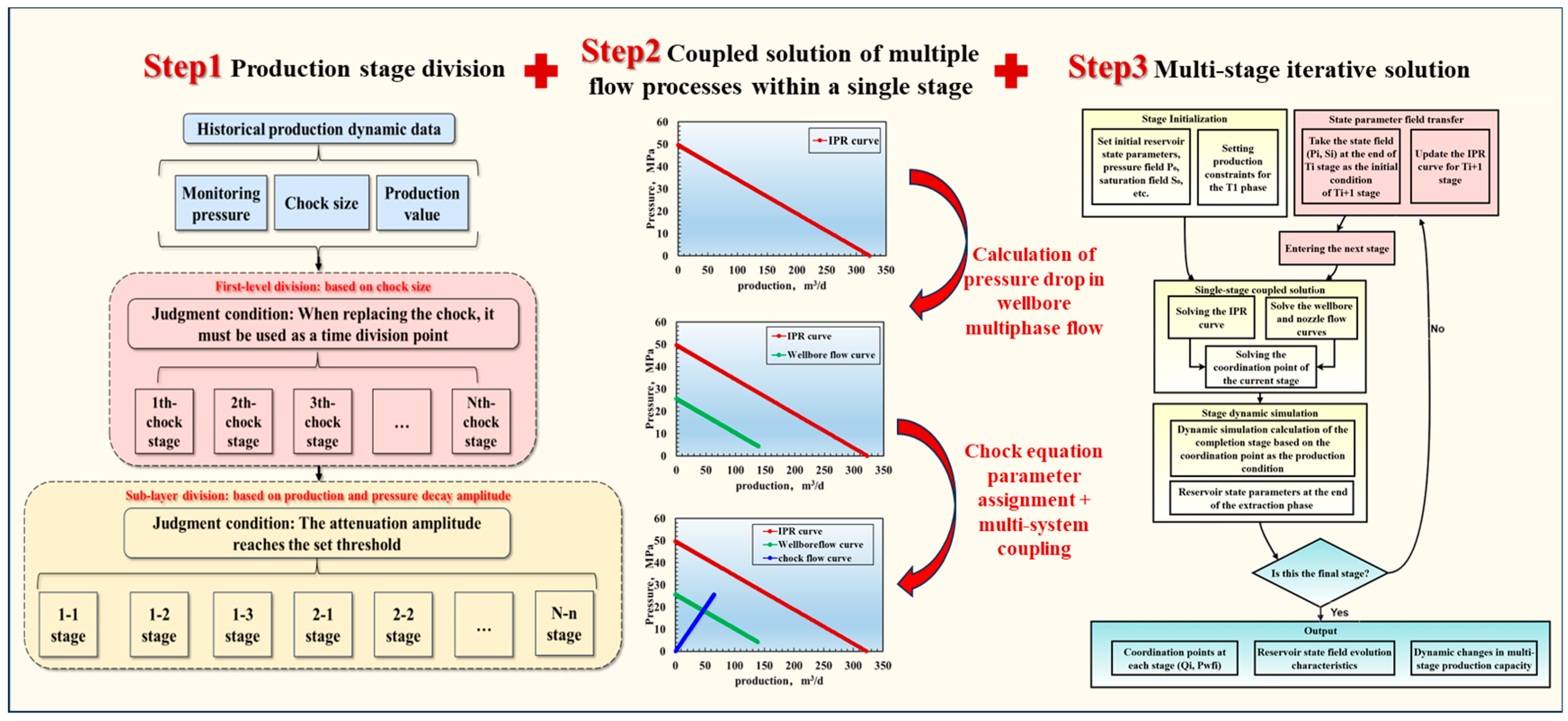
Figure 1: The basic ideas for model establishment.
The duration of the pseudo-steady-state periods is determined by analyzing the trends of key parameters within the historical production data. The main criteria are as follows: (1) The most apparent inflection points in the historical production data should correspond to the moments when the choke size was changed. Therefore, a primary principle of this method must be followed: all sub-stages must be divided based on a constant choke size; a single stage cannot span across a change in choke size. Consequently, all time points at which the choke was changed are treated as mandatory division points in this method. (2) After completing the first-level stage division based on choke size, a second level of division is required for the production periods under a single choke size. In field operations, production with a single choke size can often last for several months. During this time, even though the choke is not changed, the reservoir energy gradually depletes due to the continuous production of subsurface fluids, causing both the wellhead pressure and the production rate to decline. Therefore, a secondary division of the time period is necessary, based on the magnitude of decline of these two parameters. In the corresponding algorithm settings of this paper, the data analyst can customize the required decline threshold. Based on this threshold, the production period is further divided to obtain the final iterative solution scheme. The specific division process is as follows:
Let the time series T over the well’s production period be represented as:
Then, at each time point
From the above equation, the first-level time stages derived from the choke size division are as follows:
Building upon this, we further subdivide each stage
The respective decline magnitudes for the production rate and pressure, which are the criteria for partitioning this sub-stage, are defined as:
When either of the two reaches a set threshold, a new sub-stage is demarcated, i.e.,
In the above formula,
As shown in Fig. 2. Taking the choke size, production rate, and monitored pressure curves of a well as an example, the differently colored regions represent the primary time stages, which are partitioned based on choke size. The areas delineated by dashed lines represent the partitioning into secondary time stages within a single choke size setting. The analysis within each production stage obtained through this method can be treated as a steady-state flow. It should be noted that the 15% marked in the figure is not a fixed value. In actual calculations, the size of this threshold can be adjusted according to different working conditions. Moreover, for more precise calculation, each time period here can even be divided into one day or even one hour. However, it should be noted that this will result in a relatively long calculation time.
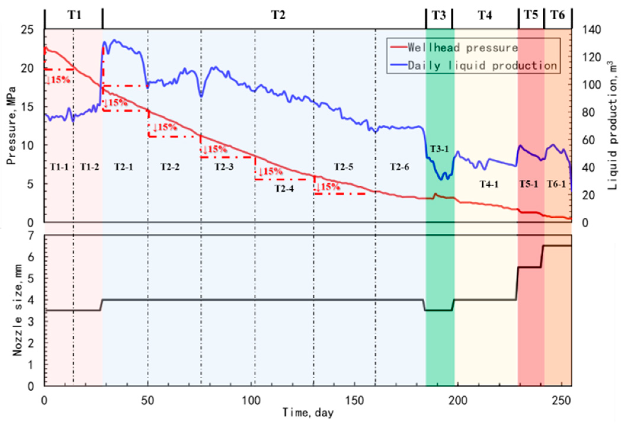
Figure 2: Schematic of production stage division.
2.2.2 Production Rate Calculation
At any given time, the production of an oil well involves three processes: flow from the reservoir to the wellbore, flow from the bottomhole to the wellhead, and outflow from the wellhead. The corresponding relationships between pressure and production rate for these three processes are as follows:
The above equation represents the Inflow Performance Relationship for the process of flow from the reservoir to the wellbore. In this equation:
Subsequently, during the flow from the bottomhole to the wellhead, the fluid’s energy is expended to overcome the hydrostatic pressure and frictional pressure drops. The relationship between the wellhead and bottomhole pressures is accordingly expressed as:
In this formula,
The choke flow curve is typically highly empirical. The applicable calculation formulas for choke flow vary with different regions and reservoir types. Currently, a widely used general formula can be expressed as:
In this formula,
In summary, Eqs. (9), (10), (11) respectively describe the three key flow processes of the reservoir, wellbore and choke in the production system. These three flow processes do not exist in isolation in actual production but are interrelated and mutually restrictive, jointly determining the production rate and pressure. When an oil well is in a stable production state, the entire flow system must simultaneously satisfy the principles of mass conservation and energy conservation of the fluid, that is, the inflow volume of the reservoir, the conveying capacity of the wellbore, and the throttling capacity of the choke need to reach a dynamic balance. The characteristic curves of the above three flow systems were plotted in the same coordinate system to study the intrinsic relationship between output and pressure corresponding to the three. During the production period of T1 stage, the gas/oil ratio R was set to 150 m3/m3 and the choke diameter d was set to 2 mm. The results are shown in Fig. 3.
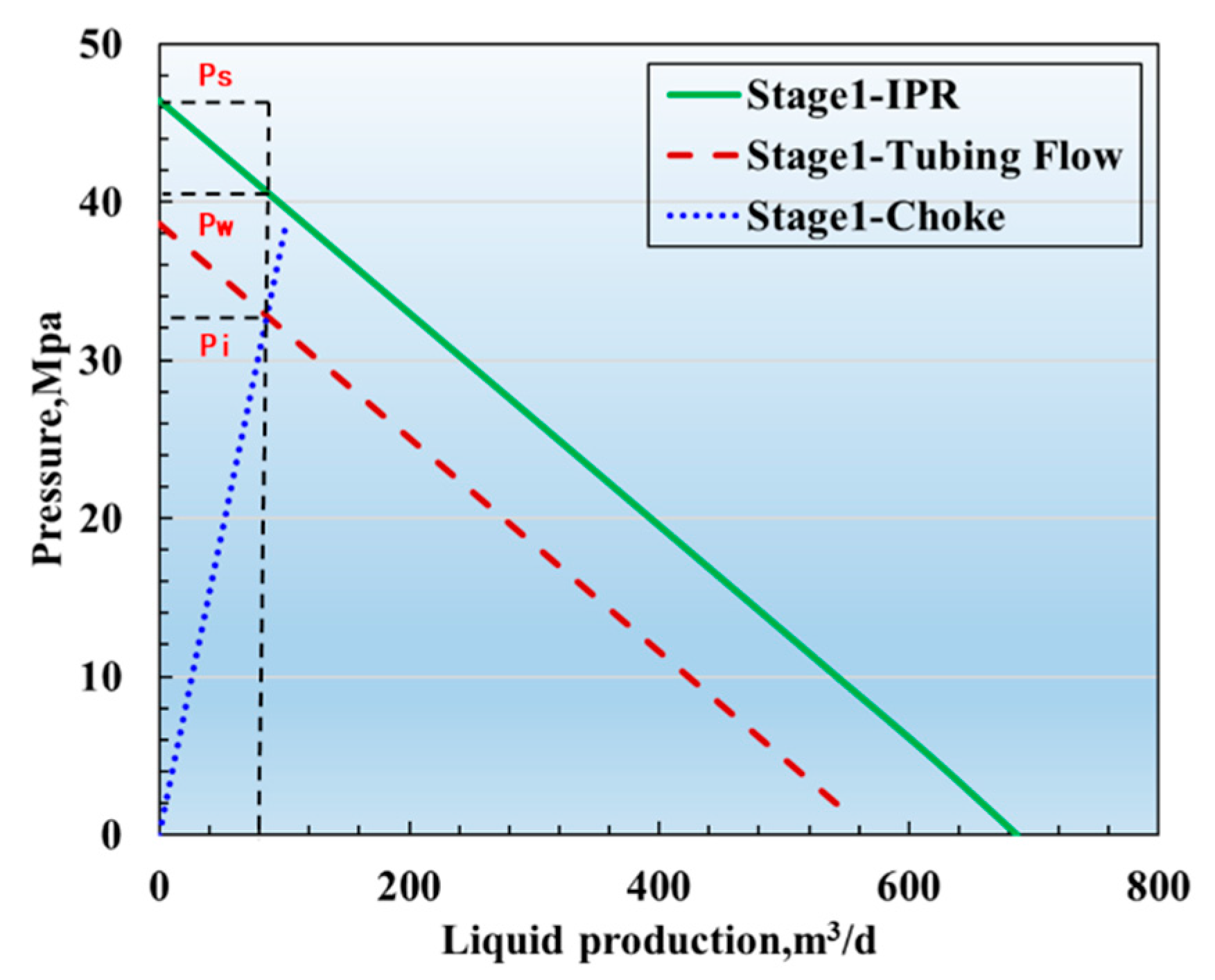
Figure 3: Three flow curves in stage T1.
It can be seen from Fig. 3 that in the T1 production stage, at the intersection of the choke flow curve (blue) and the tubing flow curve (red), the actual production rate at a 2 mm choke in this stage is 85.8 m3/d, the wellhead and bottomhole pressures corresponding to actual production are Pi and Pwf. Therefore, Ps-Pwf represents the pressure consumed by the fluid flowing from the reservoir to the wellbore, and Pwf-Pi represents the pressure consumed by the fluid flowing from the bottomhole to the wellhead in the tubing. Under the conditions of this production volume and corresponding pressure, the production of the oil well is stable, and the three flows are interconnected and coordinated. At this time, the point corresponding to the production volume is the coordination point of the T1 stage.
Based on the single-stage flow solution model, the multi-stage dynamic iterative solution process is constructed as follows:
- (1)Stage initialization:
- I.Set initial reservoir state parameters (pressure field P0, saturation field S0, etc.);
- II.T1 stage (0–20 days) production constraints;
- (2)Single-stage coupled solution:
- I.Based on the current reservoir state, solve the correspondence between different bottomhole pressure and production rate to build the IPR curve at the current stage;
- II.Build the tubing flow curve and choke flow curve based on the wellbore parameters and choke size;
- III.Solve the coordination point of the current stage (Q1, Pwf1);
- (3)Stage dynamic simulation:
- I.Complete the dynamic simulation calculation of the current stage (0–20 days) with the coordination point (Q1, Pwf1) as the production condition;
- II.Reservoir state parameters (P1, S1) at the end of the extraction stage time point (t = 20 d);
- (4)State parameter field transfer:
- I.The state field (P1, S1) at the end of T1 stage is taken as the initial condition of T2 stage;
- II.Update the IPR curve of stage T2 to reflect the dynamic changes of the reservoir;
- (5)Multi-stage iteration solution:
- I.Repeat step (2) to solve the coordination point (Q2, Pwf2) in T2 stage;
- II.Repeat step (3) to simulate T1 stage with (Q1, Pwf1) and simulate T2 stage with (Q2, Pwf2), and extract the reservoir state parameters (P2, S2) at the end of the phase (t = 40 d) time point;
- III.Repeat the steps (4) and redirect them to the subsequent production stages (T3, …, Tn);
- (6)Dynamic output:
- I.Coordination points at each stage (Qi, Pwfi);
- II.Reservoir state field evolution characteristics;
- III.Dynamic changes in multi-stage production capacity.
This solving process achieves full-cycle coupling calculation of the reservoir-wellbore-choke system through dynamic transmission and updating of inter-stage state parameters, enabling accurate characterization of the dynamic response characteristics in multi-stage production processes of shale oil reservoirs.
3 Analysis of the Necessity of Adjusting the Size of the Choke
By building a multi-stage iterative model, the previous article reveals the dynamic evolution of production capacity during the development process. In light of the actual production characteristics of shale reservoirs, during the long-term depletion development process, the application strategies of different choke sizes will lead to different production capacity performances. For instance, the use of large-sized choke can achieve a relatively high production rate in the short term, but it may lead to rapid energy consumption in the reservoir and a quick decline in production rate. Conversely, although the production of small-sized choke is limited, it can delay the pressure attenuation of the reservoir and improve the later performance. However, a single static choke system often fails to balance the dual goals of rapid initial production capacity release and stable production rate in the later stage. Therefore, the dynamic adjustment of choke is regarded as an important control measure in the optimization of shale oil reservoir development systems.
In order to further utilize the application advantages of the model and verify its response characteristics to different choke size usage strategies, this paper designs three choke management scenarios. (1) employing a large choke size throughout the entire production period for maximum-rate extraction; (2) adopting a small choke size throughout for conservative, pressure-stabilized extraction; (3) Use small choke size in the early stage and gradually replacing them with large choke size as production progresses. By comparing the stage-wise production trends and the final cumulative production under these different choke adjustment strategies, a systematic analysis of the comprehensive impact of choke management on reservoir pressure evolution, wellbore flow characteristics, and the well’s ultimate production capacity is conducted. The specific parameter settings and the results of each plan are shown in Table 1 and Table 2.
Table 1: Model parameter settings.
| Parameter | Value | Parameter | Value |
|---|---|---|---|
| Original stratigraphic pressure/MPa | 20 | Pump pressure/MPa | 80 |
| Displacement/m3/min | 15 | Fracture spacing/m | 60 |
| Number of fracturing sections | 20 | Fracture length/m | 300 |
| fracture permeability/D | 100 | Matrix permeability/mD | 0.05 |
| Vertical wellbore length/m | 1000 | Horizontal wellbore length/m | 1500 |
| Water viscosity/cp | 1 | Oil viscosity/cp | 5 |
| Water density/kg/m3 | 1000 | Oil density/kg/m3 | 800 |
| Water compressibility/bar−1 | 1 × 10⁻⁸ | Oil compressibility/bar−1 | 1 × 10⁻⁵ |
| Rock compressibility/bar−1 | 1 × 10⁻⁴ | Single-fracture fracturing time/h | 2 |
| Shut in time/day | 20 | Absolute roughness of tubing/mm | 0.02 |
| Tubing diameter/mm | 114.3 | Production time/day | 100 |
| Model length/m | 1500 | Model width/m | 500 |
Table 2: The usage of choke in different schemes.
| Stage | Production Time | Scheme 1: Extreme Production | Scheme 2: Dynamic Adjustment | Scheme 3: Conservative Production |
|---|---|---|---|---|
| Choke Size (mm) | Choke Size (mm) | Choke Size (mm) | ||
| T1 | 0–30 days | 7.5 | 2.0 | 2.0 |
| T2 | 31–60 days | 7.5 | 2.5 | 2.0 |
| T3 | 61–90 days | 7.5 | 3.0 | 2.0 |
| T4 | 91–120 days | 7.5 | 3.5 | 2.0 |
| T5 | 121–150 days | 7.5 | 4.0 | 2.0 |
| T6 | 151–180 days | 7.5 | 4.5 | 2.0 |
| T7 | 181–210 days | 7.5 | 5.0 | 2.0 |
| T8 | 211–240 days | 7.5 | 5.5 | 2.0 |
| T9 | 241–270 days | 7.5 | 6.0 | 2.0 |
| T10 | 271–300 days | 7.5 | 6.5 | 2.0 |
| T11 | 301–330 days | 7.5 | 7.0 | 2.0 |
| T12 | 331–360 days | 7.5 | 7.5 | 2.0 |
Simulation scheme of the above three groups, respectively, and obtain the following results.
Table 3, Table 4 and Table 5, Fig. 4, Fig. 5, Fig. 6, Fig. 7, Fig. 8 and Fig. 9 present the production and pressure response characteristics of the well under different choke control scenarios. The results indicate that for scheme 1, where a large choke size (7.5 mm) was used continuously, a phenomenon occurred after the T5 stage where the choke performance curve and the tubing performance curve no longer intersected. This signifies that under the prevailing bottomhole flowing pressure conditions of that stage, the reservoir could no longer support spontaneous flow with the installed choke size. Similarly, in scheme 2, despite employing a dynamic choke adjustment strategy, the same condition of no intersection point between the curves occurred after the T10 stage. Therefore, the calculated production and pressure results for the subsequent stages in these two scenarios are considered invalid and are excluded from further statistical analysis.
Table 3: The production situation at each stage of scheme 1.
| Stage | Choke Size (mm) | Production Rate (m3/d) | Bottomhole Pressure (MPa) | Wellhead Pressure (MPa) |
|---|---|---|---|---|
| T1 | 7.5 | 310.22 | 16.3 | 8.44 |
| T2 | 7.5 | 135.94 | 11.55 | 3.69 |
| T3 | 7.5 | 70.05 | 9.75 | 1.90 |
| T4 | 7.5 | 42.30 | 9.00 | 1.15 |
| T5 | - | - | - | - |
| T6 | - | - | - | - |
| T7 | - | - | - | - |
| T8 | - | - | - | - |
| T9 | - | - | - | - |
| T10 | - | - | - | - |
| T11 | - | - | - | - |
| T12 | - | - | - | - |
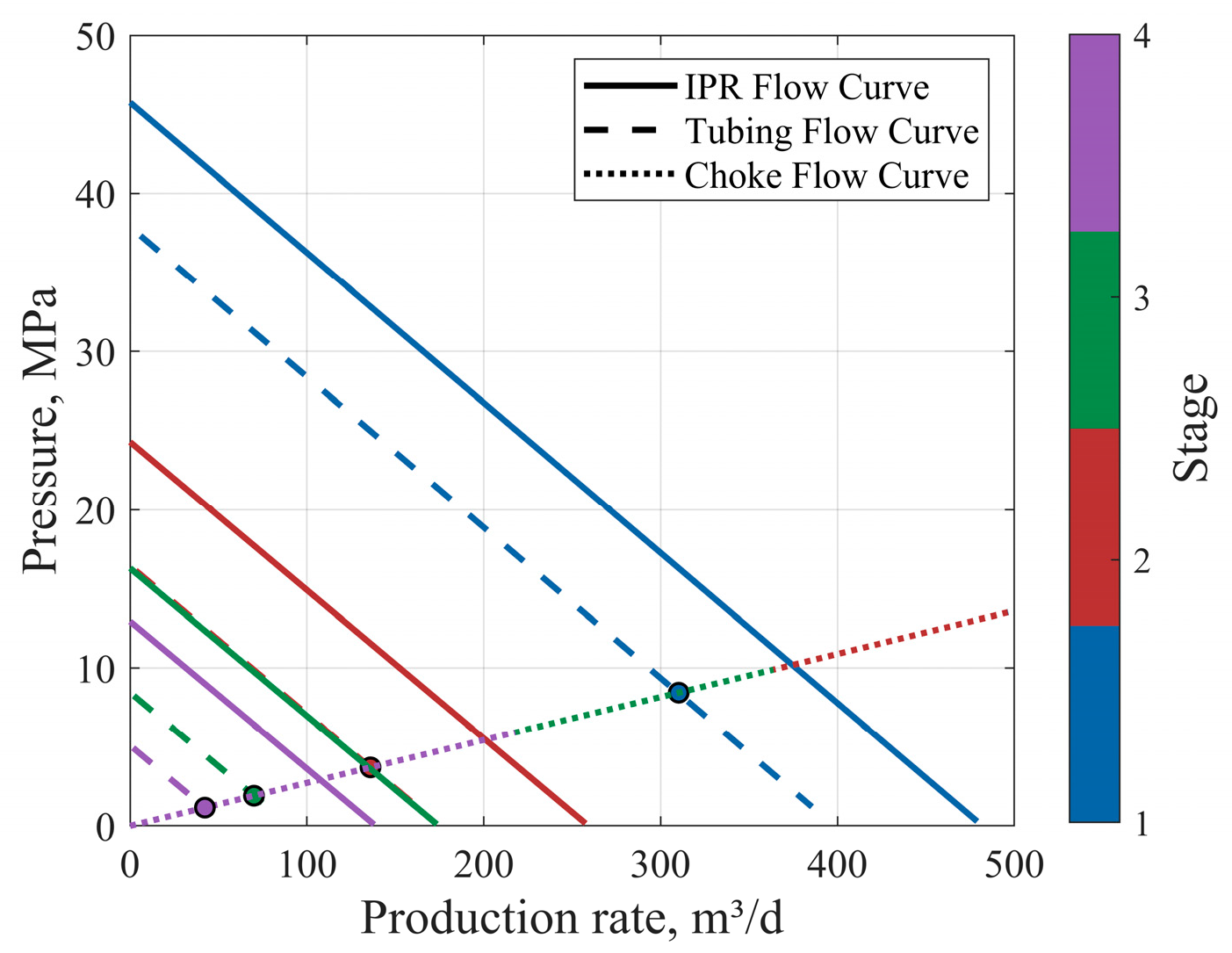
Figure 4: Flow curves at each stage (scheme 1).
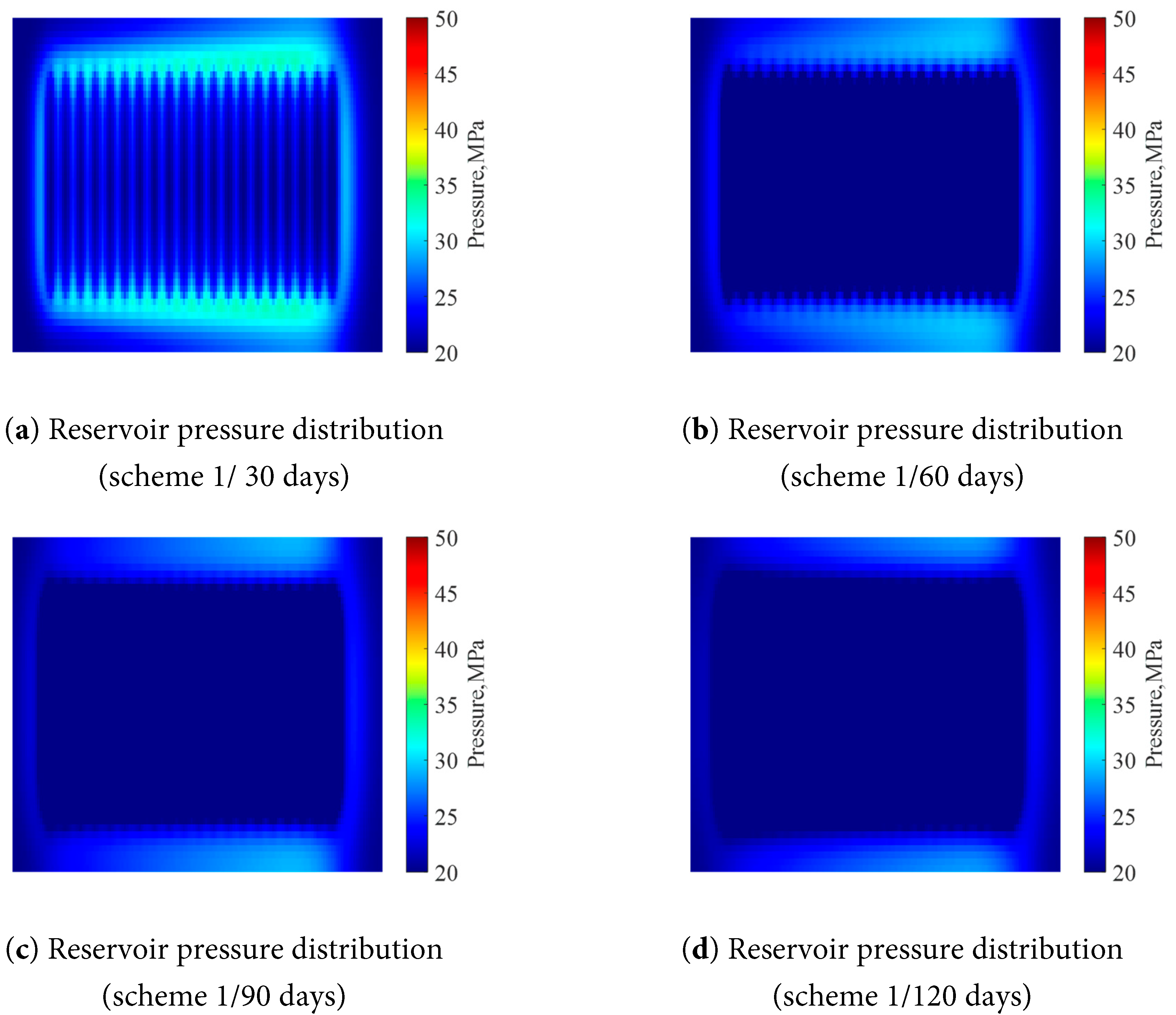
Figure 5: Pressure distribution at different production times (scheme 1).
Table 4: The production situation at each stage of scheme 2.
| Stage | Choke Size (mm) | Production Rate (m3/d) | Bottomhole Pressure (MPa) | Wellhead Pressure (MPa) |
|---|---|---|---|---|
| T1 | 2 | 79.32 | 38.21 | 30.35 |
| T2 | 2.5 | 92.34 | 30.47 | 22.62 |
| T3 | 3 | 93.67 | 23.78 | 15.93 |
| T4 | 3.5 | 85.49 | 18.53 | 10.68 |
| T5 | 4 | 72.18 | 14.75 | 6.91 |
| T6 | 4.5 | 57.94 | 12.23 | 4.38 |
| T7 | 5 | 45.42 | 10.63 | 2.78 |
| T8 | 5.5 | 35.60 | 9.65 | 1.80 |
| T9 | 6 | 28.41 | 9.06 | 1.21 |
| T10 | - | - | - | - |
| T11 | - | - | - | - |
| T12 | - | - | - | - |
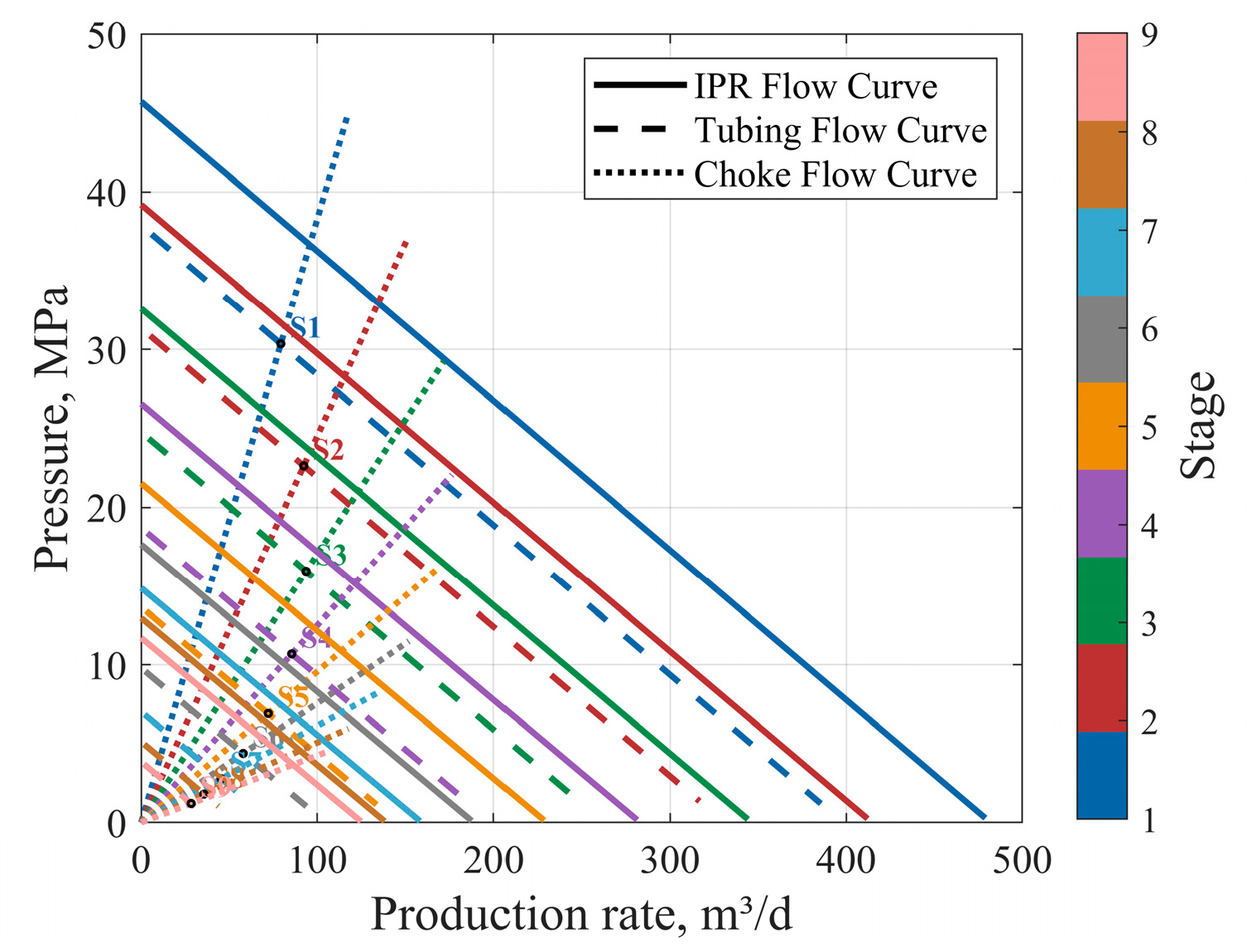
Figure 6: Flow curves at each stage (scheme 2).

Figure 7: Pressure distribution at different production times (scheme 2).
Table 5: The production situation at each stage of scheme 3.
| Stage | Choke Size (mm) | Production Rate (m3/d) | Bottomhole Pressure (MPa) | Wellhead Pressure (MPa) |
|---|---|---|---|---|
| T1 | 2 | 79.32 | 38.21 | 30.36 |
| T2 | 2 | 65.68 | 32.98 | 25.13 |
| T3 | 2 | 55.51 | 29.09 | 21.24 |
| T4 | 2 | 47.65 | 26.08 | 18.23 |
| T5 | 2 | 41.45 | 23.71 | 15.86 |
| T6 | 2 | 36.49 | 21.81 | 13.96 |
| T7 | 2 | 32.45 | 20.27 | 12.42 |
| T8 | 2 | 29.13 | 18.99 | 11.15 |
| T9 | 2 | 26.36 | 17.93 | 10.09 |
| T10 | 2 | 24.03 | 17.04 | 9.19 |
| T11 | 2 | 22.04 | 16.28 | 8.43 |
| T12 | 2 | 20.32 | 15.62 | 7.77 |
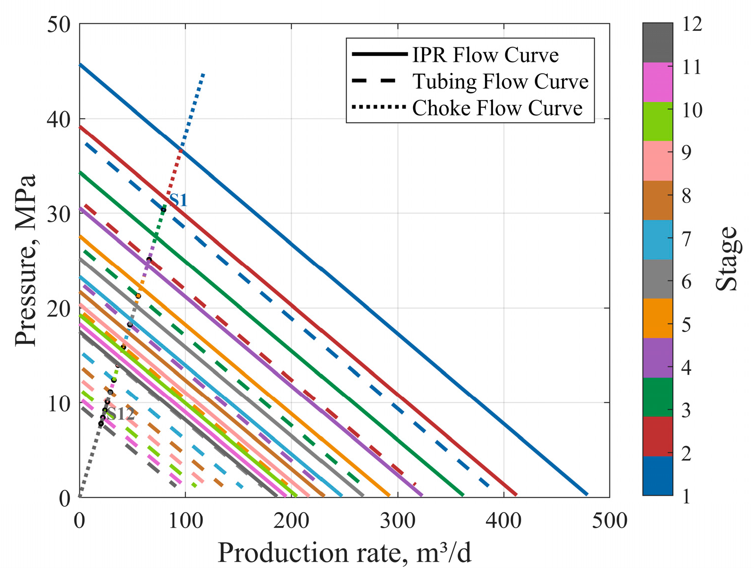
Figure 8: Flow curves at each stage (scheme 3).
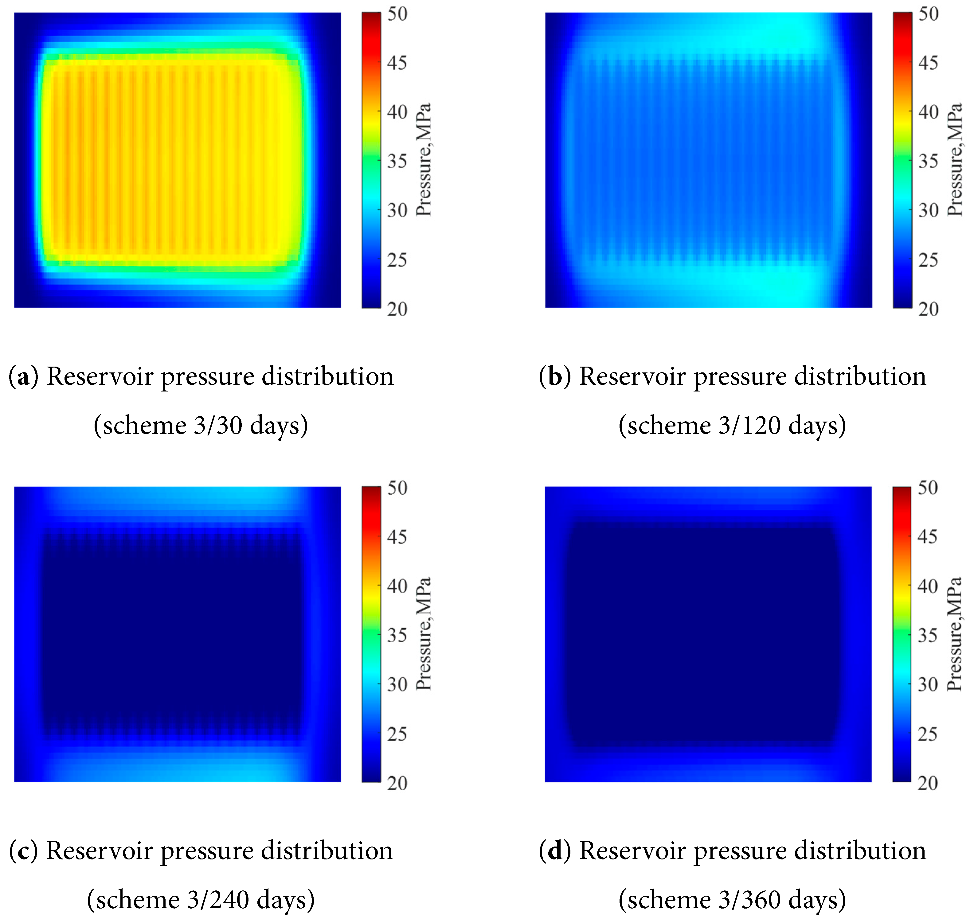
Figure 9: Pressure distribution at different production times (scheme 3).
From Fig. 10, Fig. 11 and Fig. 12, the following patterns can be observed:
- (1)In scheme 1, production was conducted using a large 7.5 mm choke. Although the initial daily production rate was high, the rate of decline was extremely rapid. It achieved a daily rate of 310.22 m3/d in the T1 stage, but in the T4 stage, this had decreased to 42.30 m3/d, after which the well could no longer sustain spontaneous flow. The cumulative effective production time accounted for only about 45% of the total production duration. This indicates that the production capacity was highly concentrated in the initial period, leading to rapid reservoir depletion in the later stages and, consequently, limiting the final cumulative production.
- (2)Scheme 3 utilized a 2 mm small choke size throughout the entire production period. The daily production rate was stable but consistently low, starting at only 79.32 m3/d in the T1 stage and decreasing to 20.32 m3/d by the T12 stage. However, the release of reservoir energy was restricted, which led to a low cumulative production and, consequently, non-ideal economic benefits.
- (3)Scheme 2 adopted a dynamic choke size strategy, which effectively balanced reservoir energy conservation with production capacity release. In the initial stage, a small choke was used to control the production rate, thereby delaying reservoir pressure decline. In the middle stage, the choke size was gradually increased to achieve a phased production enhancement. In the later stage, under conditions of low bottomhole pressure, the choke was moderately enlarged to maintain production fluidity. This approach resulted in the highest cumulative production and a well-balanced capacity release, avoiding the extremes of both “early overdraft” and “later-stage fatigue”. It successfully achieved an excellent balance between production stability and the maximization of production capacity.
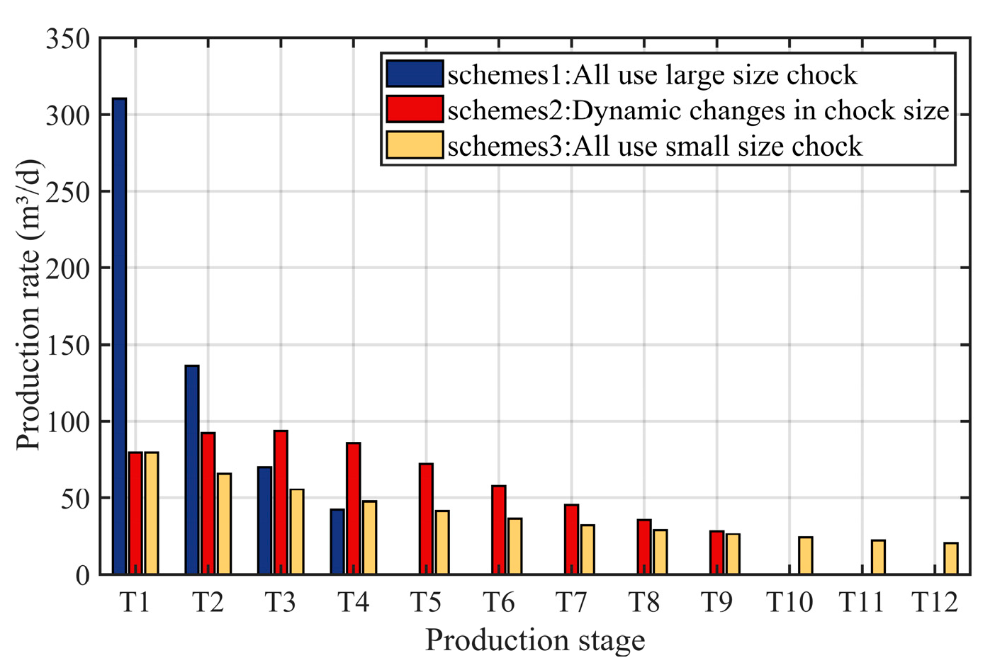
Figure 10: Comparison of daily production rate at each stage under different schemes.
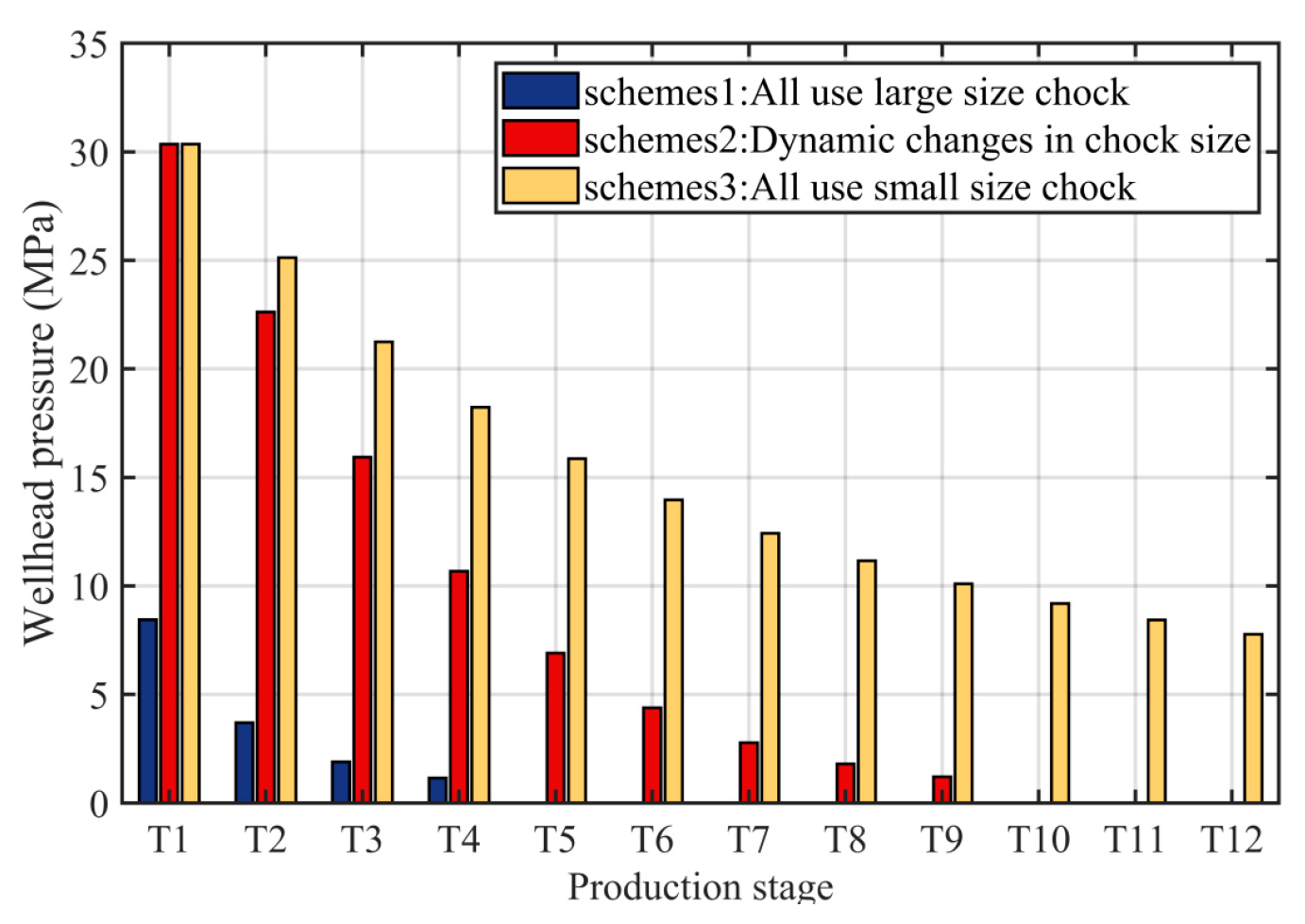
Figure 11: Comparison of wellhead pressure at each stage under different schemes.

Figure 12: Comparison of bottomhole pressure at each stage under different schemes.
We will use the previously established model to predict the dynamic production data of a fractured horizontal well in a shale oil reservoir and validate the predictions by comparing them with actual data. The data for this case were selected from a fractured horizontal well located in the tight oil-rich area of the Jimsar, in the eastern Junggar Basin. The relevant parameters for the reservoir and the hydraulic fracturing operation were sourced from the on-site operational report, as shown in Table 6.
Table 6: Parameter settings (Case 1).
| Parameter | Value | Parameter | Value |
|---|---|---|---|
| Number of fracturing sections | 30 | Number of fractures | 86 |
| Fracture length/m | 150 | Fracture aperture/m | 0.005 |
| Cluster spacing/m | 10~30 | Fracture permeability/D | 40 |
| Matrix permeability/mD | 0.01 | Fracture conductivity/mD·m | 200 |
| Original stratigraphic pressure/MPa | 33.0 | Vertical wellbore length/m | 2720 |
| Displacement/m3/min | 12~18 | Horizontal wellbore length/m | 1348 |
| Water viscosity/cp | 1 | Tubing size | 5–1/2 |
| Water density/kg/m3 | 1000 | Oil viscosity/cp | 5 |
| Water compressibility/bar−1 | 1 × 10⁻⁸ | Oil density/kg/m3 | 800 |
| Rock compressibility/bar−1 | 1 × 10⁻⁴ | Oil compressibility/bar−1 | 1 × 10⁻⁵ |
| Shut in time/day | 10 | Production time/day | 261 |
This well was shut in for 10 days after the completion of fracturing. According to the actual fracturing construction data on site, the distribution of reservoir pressure at two time points of the completion of fracturing and the completion of the shutting in was obtained through simulation, as shown in Fig. 13 and Fig. 14.
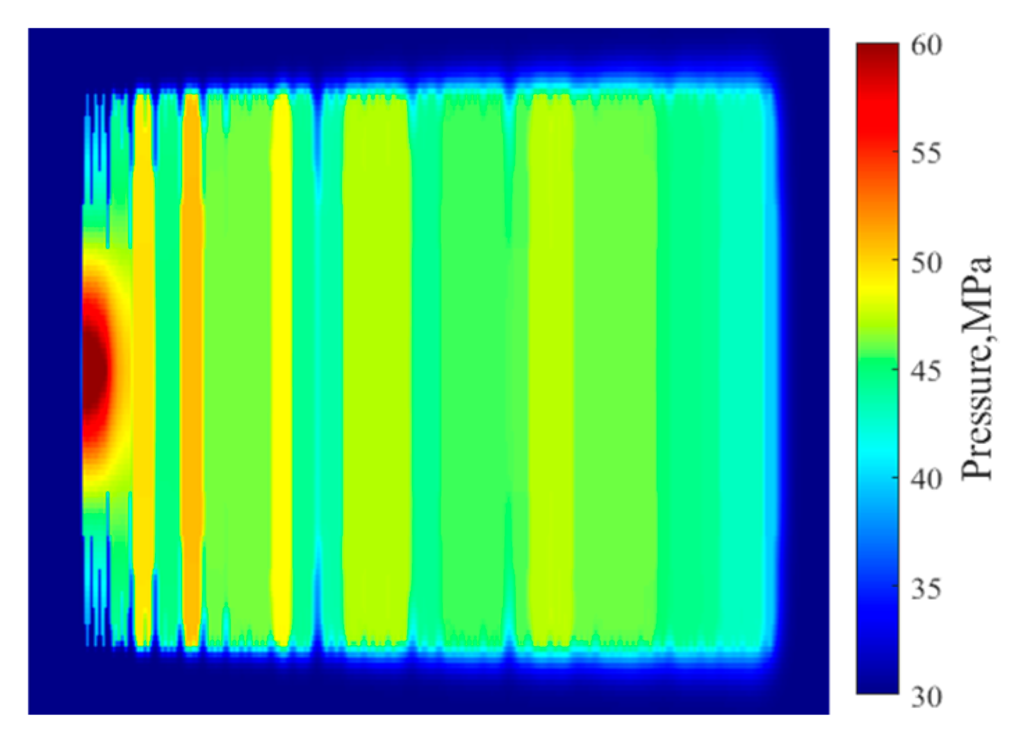
Figure 13: Pressure distribution at the end of fracturing (Case 1).
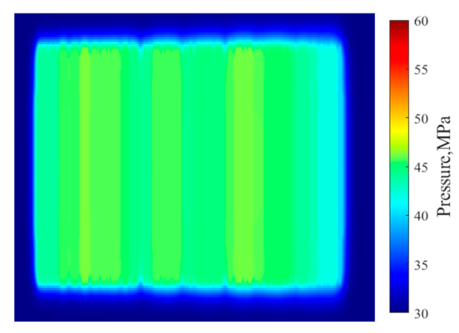
Figure 14: Pressure distribution at the end of shut-in (Case 1).
On this basis, the simulation of the production phase was continued, covering the period from the end of the shut-in until the transition to artificial lift. The spontaneous flow period lasted for 261 days, during which a total of 8 different choke sizes, ranging from 3 mm to 6.5 mm, were utilized. In order to predict and match the production dynamics of this actual reservoir with greater accuracy, this study, after comprehensive consideration, refines the simulation by dividing the entire production cycle into more granular intervals. Each day is treated as a single time step for the solution process. The production dynamics calculated in this manner further reduce the uncertainty associated with unsteady-state flow in the time dimension, ensuring that the obtained results are more consistent with field observations and understanding.
Based on the production stage division described above, the IPR curves and tubing curves were solved for each respective stage. By integrating the flow characteristics of different choke sizes, the production rates for various stages were predicted and subsequently compared with actual production data. The specific calculation results are presented below. Due to the extensive volume of daily production data, Table 7 displays the results as averaged values, calculated according to the actual choke change frequency and production decline rates. The detailed fit of the daily production data can be seen in Fig. 15. To further illustrate the threshold mentioned in the previous text, in this case, two judgment methods, namely the decline in production and the decline in wellhead pressure, were respectively used to divide the time. The reasons for the division of each stage are shown in Table 7.
It is important to note that during each step of the calculation process, the water cut gradually decreases, causing the oil-to-water ratio in the wellbore to change in real-time. Consequently, the hydrostatic pressure and frictional pressure of the fluid column, as it is lifted from the bottom of the well to the surface, also change over the course of production. The primary influencing factor in this dynamic is the density of the oil-water mixture. To accurately reflect the fluctuations in pressure loss caused by this effect, this study updates the mixed-fluid density in real-time during each solution step, corresponding to the changes in water cut.
Table 7: Reasons for the division of different stages (Case 1).
| Main Stage | Sub Stage | Production Time (Day) | Choke Size (mm) | Reasons for Stage Division |
|---|---|---|---|---|
| 1 | 1-1 | 10 | 3.5 | Wellhead pressure dropped by 10% |
| 1 | 1-2 | 10 | 3.5 | Wellhead pressure dropped by 10% |
| 1 | 1-3 | 10 | 3.5 | Replace the choke |
| 2 | 2-1 | 20 | 4.0 | Production rate dropped by 10% |
| 2 | 2-2 | 20 | 4.0 | Production rate dropped by 10% |
| 2 | 2-3 | 20 | 4.0 | Production rate dropped by 10% |
| 2 | 2-4 | 20 | 4.0 | Production rate dropped by 10% |
| 2 | 2-5 | 20 | 4.0 | Production rate dropped by 10% |
| 2 | 2-6 | 20 | 4.0 | Production rate dropped by 10% |
| 2 | 2-7 | 20 | 4.0 | Production rate dropped by 10% |
| 3 | 3-1 | 16 | 4.0 | Replace the choke |
| 4 | 4-1 | 5 | 3.5 | Replace the choke |
| 5 | 5-1 | 9 | 3.0 | Replace the choke |
| 6 | 6-1 | 21 | 4.0 | Replace the choke |
| 7 | 7-1 | 3 | 4.5 | Replace the choke |
| 8 | 8-1 | 7 | 5 | Replace the choke |
| 9 | 9-1 | 15 | 5.5 | Replace the choke |
| 10 | 10-1 | 15 | 6.5 | Production has ended |
It can be seen from the results shown in Table 8 and Table 9, it is evident that the liquid production rates calculated by the model exhibit a small error relative to the actual values throughout the entire spontaneous flow period. In a total of 13 sub-stages, the absolute error was below 5 m3/d, indicating high fitting accuracy, with an overall fitting rate exceeding 90%. A larger deviation was observed during the late production stage, which involved a gradual transition to larger choke sizes. Analysis suggests that the potential causes for this discrepancy are either that the reservoir pressure, having become excessively low after prolonged production, failed to meet the threshold required for spontaneous flow, or that the model’s production calculation was underestimated due to inaccurate parameters in the flow equation for large chokes. From the perspective of cumulative liquid production, the absolute error between the model’s calculation and the actual cumulative volume is 115.75 m3, corresponding to a relative error of only 0.56% and fitting rate reaches 97%, which demonstrates a good fitting effect. Regarding the oil production fit, the model’s performance in matching the high water cut phenomenon during the initial flowback stage was suboptimal. However, the fit normalized after the second stage, with the overall error remaining within 10%, the comprehensive fitting rate is 71%. Furthermore, the calculated cumulative oil production for the entire period was 8865.55 m3, compared to the actual cumulative oil production of 8870.43 m3, resulting in an error of merely 0.06%. Concurrently, the trend of the model-calculated wellhead pressure was highly consistent with the actually monitored wellhead pressure, and the absolute pressure error was successfully controlled to below 1 MPa throughout the entire production period. The specific fitting situations of each production indicator are shown in Fig. 15. On this basis, the author believes that the problem of poor early high water cut fitting should be addressed by starting from several issues: (1) the non-Darcy flow mechanism in the flowback stage, (2) the saturation distribution in the near-wellbore zone at the initial flowback stage, and (3) further refinement of the fracture grid in the near-wellbore zone.
Table 8: Comparison of liquid production rate and error analysis (Case 1).
| Main Stage | Sub Stage | Production Time (day) | Choke Size (mm) | Actual Production Rate (m3/d) | Calculated Production Rate (m3/d) | Absolute Error (m3/d) |
|---|---|---|---|---|---|---|
| 1 | 1-1 | 10 | 3.5 | 69.1 | 83.67 | 14.57 |
| 1 | 1-2 | 10 | 3.5 | 77.2 | 81.49 | 4.29 |
| 1 | 1-3 | 10 | 3.5 | 81.5 | 79.74 | −1.76 |
| 2 | 2-1 | 20 | 4.0 | 126.6 | 129.98 | 3.38 |
| 2 | 2-2 | 20 | 4.0 | 103.0 | 120.61 | 17.61 |
| 2 | 2-3 | 20 | 4.0 | 106.5 | 111.28 | 4.78 |
| 2 | 2-4 | 20 | 4.0 | 100.2 | 101.87 | 1.67 |
| 2 | 2-5 | 20 | 4.0 | 91.7 | 92.32 | 0.62 |
| 2 | 2-6 | 20 | 4.0 | 83.0 | 82.57 | −0.43 |
| 2 | 2-7 | 20 | 4.0 | 70.3 | 72.60 | 2.3 |
| 3 | 3-1 | 16 | 4.0 | 68.7 | 64.27 | −4.43 |
| 4 | 4-1 | 5 | 3.5 | 48.7 | 37.31 | −11.39 |
| 5 | 5-1 | 9 | 3.0 | 34.2 | 32.74 | −1.46 |
| 6 | 6-1 | 21 | 4.0 | 45.0 | 49.47 | 4.47 |
| 7 | 7-1 | 3 | 4.5 | 43.1 | 39.03 | −4.07 |
| 8 | 8-1 | 7 | 5 | 47.6 | 43.12 | −4.48 |
| 9 | 9-1 | 15 | 5.5 | 50.3 | 40.02 | −10.28 |
| 10 | 10-1 | 15 | 6.5 | 48.5 | 24.60 | −23.9 |
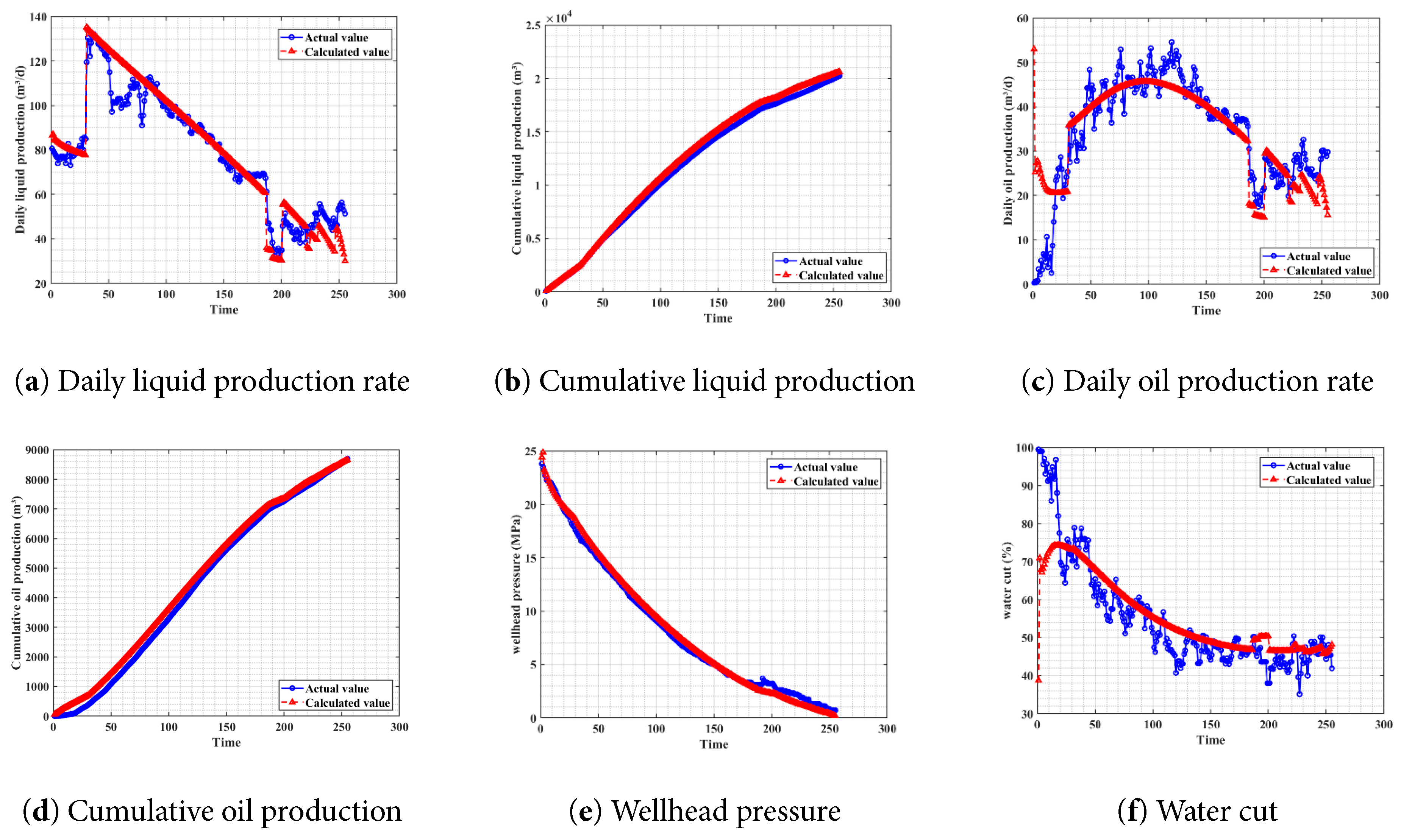
Figure 15: The fitting situation of different production indicators (Case 1).
Table 9: Fitting rates of different production indicators (Case 1).
| Index | Daily Liquid Production Rate | Cumulative Liquid Production | Daily Oil Production Rate | Cumulative Oil Production | Wellhead Pressure | Water Cut |
|---|---|---|---|---|---|---|
| R2 | 0.91 | 0.97 | 0.71 | 0.88 | 0.98 | 0.69 |
To further verify the applicability of this method, we selected another fractured horizontal well within the same oilfield and calculated its production indicators during the natural flow period. Fig. 16 and Fig. 17 show the pressure distribution status of this well at the end of fracturing and the end of shut-in. The results were then compared with the actual monitoring data. Table 10 presents the detailed parameters of Case 2.
Table 10: Parameter settings (Case 2).
| Parameter | Value | Parameter | Value |
|---|---|---|---|
| Number of fracturing sections | 32 | Number of fractures | 93 |
| Fracture length/m | 150 | Fracture aperture/m | 0.005 |
| Cluster spacing/m | 8–20 | Fracture permeability/D | 20 |
| Matrix permeability/mD | 0.01 | Fracture conductivity/mD·m | 100 |
| Original stratigraphic pressure/MPa | 35 | Vertical wellbore length/m | 3000 |
| Displacement/m3/min | 12~18 | Horizontal wellbore length/m | 1390 |
| Water viscosity/cp | 1 | Tubing size | 5-1/2 |
| Water density/kg/m3 | 1000 | Oil viscosity/cp | 5 |
| Water compressibility/bar−1 | 1 × 10⁻⁸ | Oil density/kg/m3 | 800 |
| Rock compressibility/bar−1 | 1 × 10⁻⁴ | Oil compressibility/bar−1 | 1 × 10⁻⁵ |
| Shut in time/day | 48 | Production time/day | 185 |
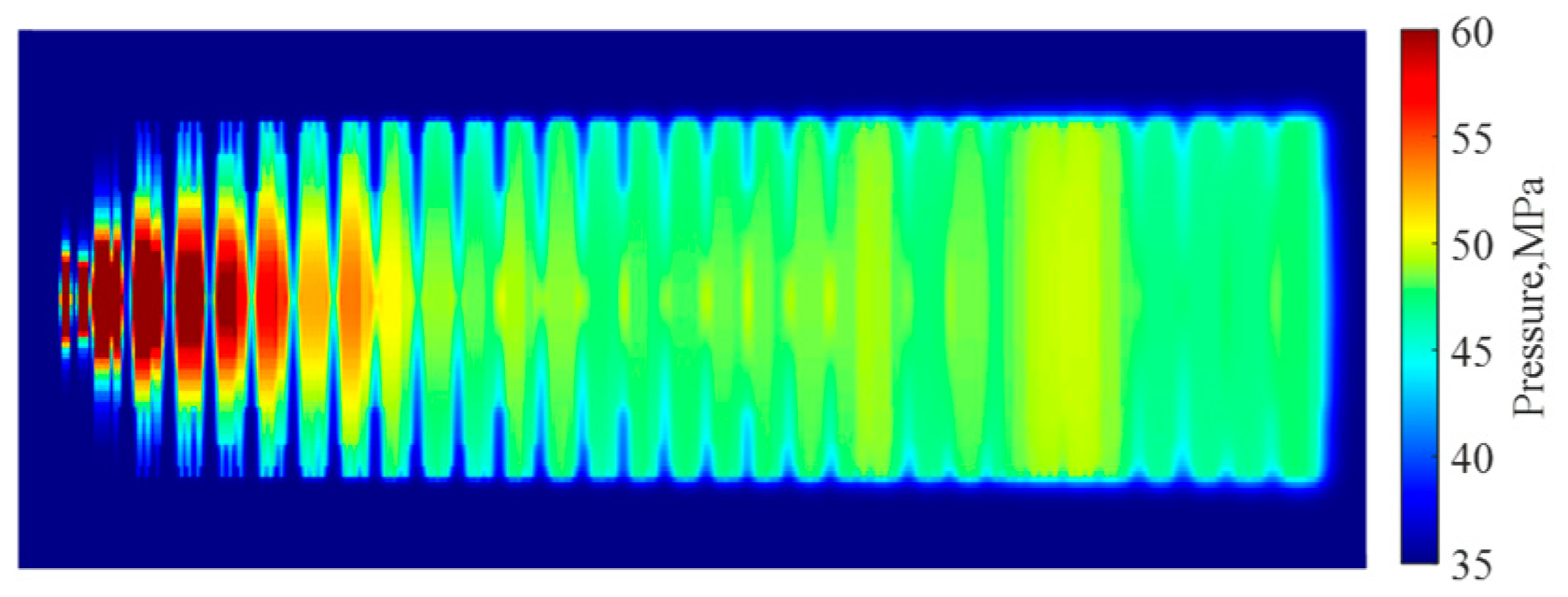
Figure 16: Pressure distribution at the end of fracturing (Case 2).
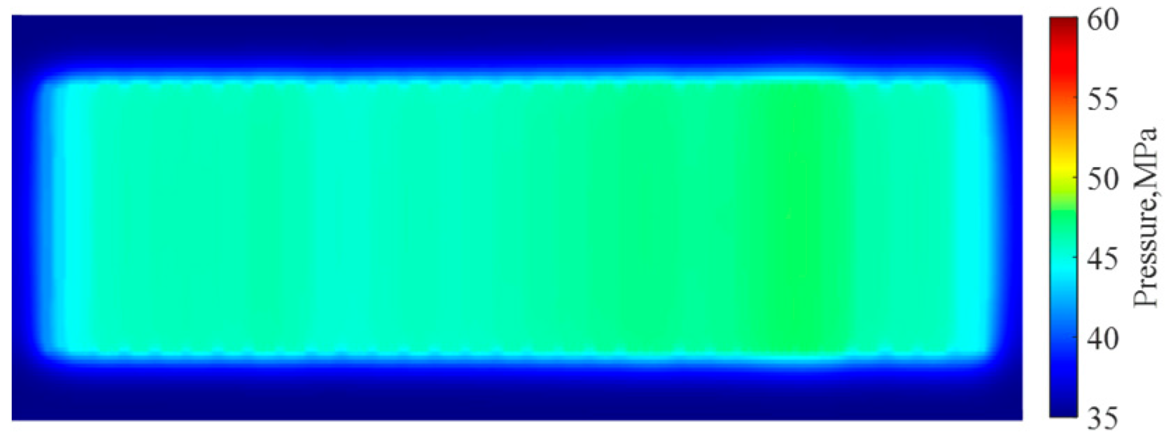
Figure 17: Pressure distribution at the end of shut-in (Case 2).
Fig. 18 and Table 11 illustrate that the fitting accuracy for the daily liquid production rate, cumulative liquid production, cumulative oil production, and wellhead pressure all exceed 90%. Due to significant fluctuations, the fitting rates for daily oil production and water cut are approximately 70%, which may be further optimized in subsequent research. Case 2 further corroborates the applicability of the method proposed in this study.
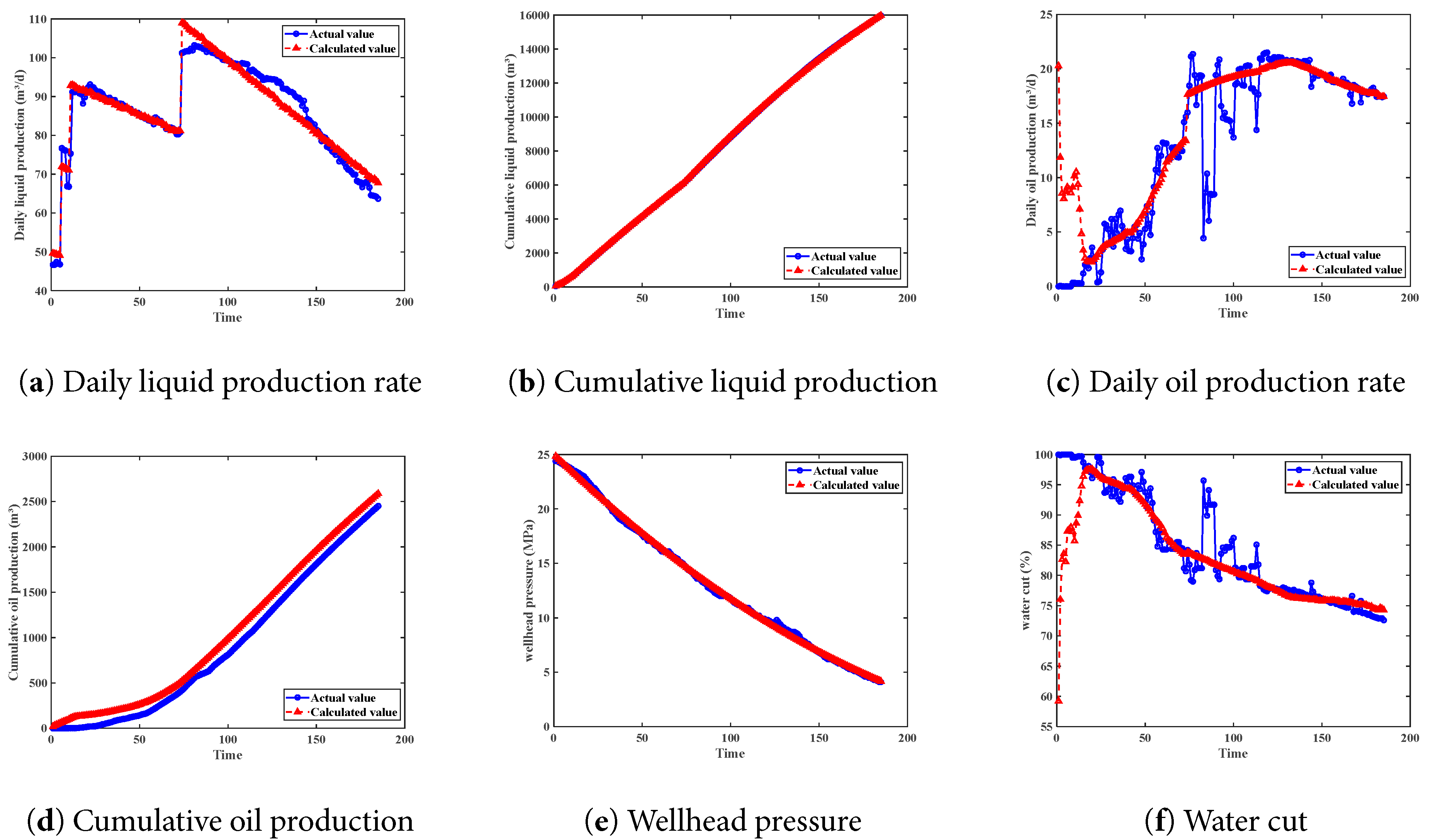
Figure 18: The fitting situation of different production indicators (Case 2).
Table 11: Fitting rates of different production indicators (Case 2).
| Index | Daily Liquid Production Rate | Cumulative Liquid Production | Daily Oil Production Rate | Cumulative Oil Production | Wellhead Pressure | Water Cut |
|---|---|---|---|---|---|---|
| R2 | 0.94 | 0.97 | 0.76 | 0.9 | 0.98 | 0.66 |
- (1)This approach involves dividing the long-term production stage into numerous short-duration sub-stages. Within these brief timeframes, the changes in reservoir fluid and energy distribution are relatively gradual, making it possible to assume that the calculations for each stage follow the principles of steady-state flow.
- (2)The calculation within a single stage should follow the nodal analysis theory. Starting from the inflow performance relationship and obtaining the corresponding relationship between production and pressure. Then, combined with the wellbore pressure calculation method, the corresponding wellhead pressure should be calculated. Finally, the actual production and pressure corresponding to the coordination point of this stage should be determined through the choke flow equation.
- (3)To handle the connection between different production stages, we strictly follow the principle of state continuity. This model uses a multi-stage, iterative simulation approach. Once we calculate the balanced production rate for a given stage, we use that data to run the simulation for that stage again. This second run gives us the true distribution of pressure and fluids in the reservoir at the end of that stage. We then use this true state as the starting point for simulating the next stage.
- (4)For the method proposed in this paper, we selected two horizontal wells in the Jimsar shale oil reservoir, modeled the fracturing period, and completed the production index calculation for the natural flow period. After comparing the calculation results with the real monitoring data, it was found that the overall fitting rates of the two cases could both reach 90%.
Acknowledgement:
Funding Statement: This work was supported by National Natural Science Foundation of China (Grant No. 52474029), National Natural Science Foundation for Young Scientists of China (A) (Grant No. 52525403), National Major Science and Technology Projects under the 14th Five-Year Plan (Grant No. 2024ZD1405105), Science and Technology Innovation Team Project of Xinjiang Uygur Autonomous Region (Grant No. 2024TSYCTD0018), Xinjiang Uygur Autonomous Region.
Author Contributions: The authors confirm contribution to the paper as follows: Related Background Research, Hui Zhao; Data collection, Guanglong Sheng; Algorithm compilation, Sheng Lei; Result analysis, Sheng Lei; Paper writing, Sheng Lei. All authors reviewed the results and approved the final version of the manuscript.
Availability of Data and Materials: The data that support the findings of this study are available upon reasonable request from the authors.
Ethics Approval: Not applicable.
Conflicts of Interest: The authors declare no conflicts of interest to report regarding the present study.
References
1. Rawlins B , Lee E , Schellhardt MA . Back-pressure data on natural-gas wells and their application to production practices. Vol. 7. Baltimore, MD, USA: Lord Baltimore Press; 1935. doi:10.55274/R0010239. [Google Scholar] [CrossRef]
2. Weller WT . Reservoir performance during two-phase flow. J Petrol Technol. 1966; 18( 2): 240– 6. doi:10.2118/1334-pa. [Google Scholar] [CrossRef]
3. Vogel JV . Inflow performance relationships for solution-gas drive wells. J Petrol Technol. 1968; 20( 1): 83– 92. doi:10.2118/1476-pa. [Google Scholar] [CrossRef]
4. Standing MB . Inflow performance relationships for damaged wells producing by solution-gas drive. J Petrol Technol. 1970; 22( 11): 1399– 400. doi:10.2118/3237-pa. [Google Scholar] [CrossRef]
5. Fetkovich MJ . The isochronal testing of oil wells. In: SPE Annual Technical Conference and Exhibition. Richardson, TX, USA: SPE; 1973. doi:10.2118/4529-MS. [Google Scholar] [CrossRef]
6. Cheng AM . Inflow performance relationships for solution-gas-drive slanted/horizontal wells. In: Proceedings of the SPE Annual Technical Conference and Exhibition; 1990 Sep 23–26; New Orleans, LA, USA. doi:10.2118/20720-MS. [Google Scholar] [CrossRef]
7. Cullender MH . The isochronal performance method of determining the flow characteristics of gas wells. Trans AIME. 1955; 204( 1): 137– 42. doi:10.2118/330-g. [Google Scholar] [CrossRef]
8. Brar GS , Aziz K . Analysis of modified isochronal tests to predict the stabilized deliverability potential of gas wells without using stabilized flow data (includes associated papers 12933, 16320 and 16391). J Petrol Technol. 1978; 30( 2): 297– 304. doi:10.2118/6134-pa. [Google Scholar] [CrossRef]
9. Stalgorova E , Mattar L . Analytical model for unconventional multifractured composite systems. SPE Reserv Eval Eng. 2013; 16( 3): 246– 56. doi:10.2118/162516-pa. [Google Scholar] [CrossRef]
10. Stalgorova E , Mattar L . Practical analytical model to simulate production of horizontal wells with branch fractures. In: Proceedings of the SPE Canadian Unconventional Resources Conference; 2012 Oct 30–Nov 1; Calgary, AB, Canada. doi:10.2118/162515-ms. [Google Scholar] [CrossRef]
11. Shahamat MS , Tabatabaie SH , Mattar L , Motamed E . Inflow performance relationship for unconventional reservoirs (transient IPR). In: Proceedings of the SPE/CSUR Unconventional Resources Conference; 2015 Oct 20–22; Calgary, AB, Canada. doi:10.2118/175975-ms. [Google Scholar] [CrossRef]
12. Ilk D , Rushing JA , Perego AD , Blasingame TA . Exponential vs. hyperbolic decline in tight gas sands—understanding the origin and implications for reserve estimates using arps&apos decline curves. In: Proceedings of the SPE Annual Technical Conference and Exhibition; 2008 Sep 21–24; Denver, CO, USA. doi:10.2118/116731-ms. [Google Scholar] [CrossRef]
13. Duong AN . An unconventional rate decline approach for tight and fracture-dominated gas wells. In: Proceedings of the Canadian Unconventional Resources and International Petroleum Conference; 2010 Oct 19–21; Calgary, AB, Canada. doi:10.2118/137748-ms. [Google Scholar] [CrossRef]
14. Duong AN . Rate-decline analysis for fracture-dominated shale reservoirs: part 2. In: Proceedings of the SPE/CSUR Unconventional Resources Conference—Canada; 2014 Sep 30–Oct 2; Calgary, AB, Canada. doi:10.2118/171610-ms. [Google Scholar] [CrossRef]
15. Ambrose RJ , Clarkson CR , Youngblood J , Adams R , Nguyen P , Nobakht M , et al. Life-cycle decline curve estimation for tight/shale reservoirs. In: Proceedings of the SPE Hydraulic Fracturing Technology Conference; 2011 Jan 24–26; The Woodlands, TX, USA. doi:10.2118/140519-ms. [Google Scholar] [CrossRef]
16. Bai W , Cheng S , Wang Y , Cai D , Guo X , Guo Q . A transient production prediction method for tight condensate gas wells with multiphase flow. Petrol Explor Dev. 2024; 51( 1): 172– 9. doi:10.1016/s1876-3804(24)60014-5. [Google Scholar] [CrossRef]
17. Li JC , Yuan B , Clarkson CR , Tian JQ . A semi-analytical rate-transient analysis model for light oil reservoirs exhibiting reservoir heterogeneity and multiphase flow. Petrol Sci. 2023; 20( 1): 309– 21. doi:10.1016/j.petsci.2022.09.021. [Google Scholar] [CrossRef]
18. Wang L , Li Q , Ran H , Pen Y . Prediction of production in multiple clusters stages fracturing horizontal well by support vector machine. In: Proceedings of the 2014 Fifth International Conference on Intelligent Systems Design and Engineering Applications; 2014 Jun 15–16; Changsha, China. p. 722– 5. doi:10.1109/isdea.2014.164. [Google Scholar] [CrossRef]
19. Luo G , Tian Y , Sharma A , Ehlig-Economides C . Eagle ford well insights using data-driven approaches. In: Proceedings of the International Petroleum Technology Conference; 2019 Mar 26–28; Beijing, China. doi:10.2523/iptc-19260-ms. [Google Scholar] [CrossRef]
20. Lee SY , Mallick BK . Bayesian hierarchical modeling: application towards production results in the eagle ford shale of south Texas. Sankhya B. 2022; 84( 1): 1– 43. doi:10.1007/s13571-020-00245-8. [Google Scholar] [CrossRef]
21. Li JH , Qin SL , Wang J , Liang CG , Chen YW , Hu K . Application of random forest algorithm in Jimsar shale reservoir. J Yangtze Univ Nat Sci Ed. 2023; 20( 2): 69– 76. doi:10.16772/j.cnki.1673-1409.20230106.001. (In Chinese). [Google Scholar] [CrossRef]
22. Wang Y , Lei Z , Zhou Q , Liu Y , Xu Z , Wang Y , et al. A physical constraint-based machine learning model for shale oil production prediction. Phys Fluids. 2024; 36( 8): 086624. doi:10.1063/5.0222243. [Google Scholar] [CrossRef]
23. Bhattacharyya S , Vyas A . Application of machine learning in predicting oil rate decline for Bakken shale oil wells. Sci Rep. 2022; 12( 1): 16154. doi:10.1038/s41598-022-20401-6. [Google Scholar] [CrossRef]
Cite This Article
 Copyright © 2025 The Author(s). Published by Tech Science Press.
This work is licensed under a Creative Commons Attribution 4.0 International License , which permits unrestricted use, distribution, and reproduction in any medium, provided the original work is properly cited.
 Downloads
 Citation Tools