Modeling of Thermal Shock-Induced Fracture Propagation Based on Phase-Field Approach

1  Introduction

Hydraulic fracturing is considered the most effective stimulating treatment to enhance gas production in deep shale due to its ultra-low permeability and high in-situ stress characteristics [1,2]. The injection of cold fracturing fluid into high-temperature formations leads to a rapid decrease in downhole temperature, potentially causing mechanical damage and failure in shale rock [3–5]. This thermal shock effect is believed to enhance the propagation of complex hydraulic fractures [6,7], leading to the proposal of cryogenic fracturing techniques in deep shale stimulation and Enhanced Geothermal System (EGS) [8,9].

Scholars have recognized that thermal shock can compromise rock strength and induce numerous micro-cracks within rock samples, as evidenced by rock mechanical experiments [10–16] observed during liquid nitrogen fracturing experiments in Eagle Ford shale that the rapid cooling of nitrogen leads to the formation of micro-cracks, significantly enhancing the permeability of the rock samples. Wu et al. [17] further observed through triaxial experiments that liquid nitrogen can markedly reduce the breakdown pressure under formation temperature conditions. Guo et al. [18] found that thermal shock activates shale bedding and the cracks induced by rapid cooling of fracturing fluid can enhance deep shale gas extraction. Li et al. [19] investigated the thermal shack damage failure modes of shale under varying contact temperature difference, cooling modes and shale bedding conditions, proposing a thermal shock index to assess the extent of thermal shock damage to shale. Lu et al. [20] investigated the influence of the contact temperature difference between the treatment fluid and the rock on thermal shock damage, identifying that a critical temperature difference of 130°C for thermal shock damage, which is associated with a significant increase in the matrix permeability of rock samples.

Given the challenges associated with experimentally revealing the mechanisms of thermal shock damage, scholars have integrated numerical simulation to investigate thermal shock cracking behaviors. Yao et al. [21] utilized Finite Element Method (FEM) based TOUGH2-EGS simulator to simulate the cryogenic fracturing process, examining the effects of temperature differences, confining pressure and injection rate on the morphology of thermal shock cracks. Sun et al. [22] developed a Finite-Discrete Element Method (FDEM) model to explore the impact of thermal shock on the fracture-induced stress field and fracture propagation within thermal anisotropic shale. Tang et al. [23] compared the distribution of fracture-induced stress and crack morphology under varying thermal shock conditions, revealing that increasing the fluid heat transfer coefficient enhances newly formed thermal shock fracture density. Liu et al. [24] and Guo et al. [25] analyzed the thermal shock cracking mechanism by establishing THM (Thermo-Hydro-Mechanical) coupled models, proposing that thermal shock facilitated fracture initiation and increased fracture complexity. While these THM-coupled models demonstrate the mechanism by which thermal shock affects the fracture induced stress field, thereby facilitating fracture initiation and propagation. Challenges remain in accurately describing complex fracture morphology due to the limitations of these approaches in dealing with sharp discontinuous fracture surfaces [26].

The continuum phase-field method is distinguished by its unique diffusion approach, which effectively simulates complex fractures growth within a multi-physics coupling environment. This method enables the characterization of fracture propagation without the necessity of tracking the fracture surface or applying additional treatments to the fracture tip [27–29]. Chu et al. [30] and Liu et al. [31] developed a THM coupled phase field model based on a framework of thermodynamic consistency. They observed the bifurcation behavior of cracks induced by thermal shock and noticed the influence of mineral anisotropy within rock samples on thermal shock damage. Yi et al. [32] focused on the influence of thermal shock on the interaction pattern between hydraulic fracture and natural fracture, and gained the key factors controlling fracture interaction. Li et al. [33] further investigate thermos-poroelastic coupling effect in the phase-field model to analyze crack growth driven mainly by thermal effects. He et al. [34,35] proposed an adaptive dynamic PFM for simulating thermoelastic fracture propagation. This innovative method addresses mixed-mode, both Mode-I and Mode-II, fracture simulation within a multi-physics environment, significantly reducing computational costs. Si et al. [36] introduced the cohesive zone method into their PFM (PF-CZM), to simulate mixed-mode crack nucleation and growth in isotropic rock subjected to thermal shock conditions. This method is believed to be effective in capturing the complex interaction behaviors of multiple cracks induced by thermal shock.

While these numerical studies have validated the detrimental effects on thermal shock on rock structures and their mechanical properties, as well as the necessity of factoring in thermal shock impacts for deep fracturing simulations, further research is required to restore the influence of in-situ conditions. Actually, the fracturing fluid injection process involves the gradual heating of the fluid within the long interval by the high-temperature formation deep formation, the fluid temperature in the fracture should be treated as a dynamic temperature. Furthermore, the damaging effects of thermal shock on the mechanically weak surfaces of shale bedding require further clarification, as this will influence the prediction of hydraulic fracture morphology. This paper presents a THM-coupled fracture propagation model based on the phase field method to simulate thermal shock-induced fracture propagation in deep shale. The governing equations and derivation process are introduced in Section 2, followed by a description of the numerical solution and model validation process in Section 3. Section 4 explores thermal shock damage under various fracture fluid temperature and pressure conditions, as well as thermal shock-induced fracture interactions within bedding planes of deep shale in the last section.

2  Mathematical Model

2.1 Thermo-Poroelastic Media Phase-Field Model

Fig. 1 illustrates the THM-coupled fracture phase-field evolution model, where a regularised diffusive fracture Гd propagates over time in a continuous medium Ω. The system includes an internal heat source S within the medium. The model’s outer boundary ∂Ω consists of the flow boundary ∂ΩP/∂Ωq, the thermal boundary ∂ΩT/ΩJ, and the mechanical boundary ∂Ωu/∂Ωt.

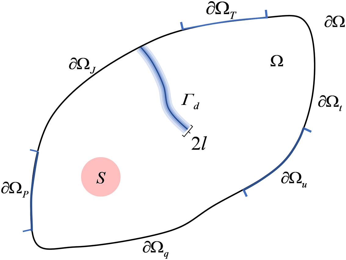
Figure 1: Diagram of a diffusive fracture in the THM coupled model

According to the variational model for quasi-static fracture [37], the total potential energy of the diffusive fracture can be represented as:

ψtotal=ψkin+ψint−ψext−ψtherm (1)

where ψkin, ψint, ψext, ψtherm are the kinetic energy, internal energy, external force work, and thermal energy, respectively. Since the model is the quasi-static model, the statement of the energy balance in the system can be written as [30]:

ψ˙kin+ψ˙int=ψ˙ext+ψ˙therm (2)

where ψ˙kin,ψ˙int denote the rate of change of kinetic energy change rate and internal energy change, respectively, ψ˙ext,ψ˙therm are the rate of work by the external forces and thermal sources. And the rate of change of kinetic energy can be expressed as:

ψ˙kin(u˙)=ddt∫Ω12ρu˙⋅u˙dV (3)

where u is the displacement tensor. And the external force work of the system is composed of the body force b and the surface force t:

ψ˙ext=∫Ωb∗⋅u˙dV+∫∂Ωtt∗⋅u˙dA (4)

where b*, t* are the body force and the traction. The work generated by the heat source and heat flux to the system can be expressed as:

ψ˙therm=−∫∂ΩTJ⋅ndA−∫∂ΩJJ¯dA+∫ΩSdV (5)

In the above equation, the first two terms represent the rate of work provided by heat flux from boundary, the heat flux tensor J term represents the work at the constant temperature boundary, the heat flux J¯ represents work at the prescribed heat flux boundary, and S represents the heat source. The last term represents the rate of work provided by heat source. n is the outward unit normal vector of the boundary surface. This paper assumes that the heat energy generated by the heat sources and temperature variation of the matrix, the heat generated by deformation and fracture of the body is not considered. The change rate of the internal energy mainly consists of three parts:

ψ˙int=ψ˙bulk+ψ˙frac+ψ˙T (6)

The three terms of the right side of the equation represent the rates of change of bulk energy, crack surface energy, as well as the thermal energy. The bulk energy consists of the elastic energy of the solid parts and the porous fluid in the matrix, with further details available in the literature [38].

ψbulk=ψe+ψf (7)

Thus, the rate of change of the bulk energy can be expressed as:

ψ˙bulk=∂ψe∂εeεe˙+∂ψe∂dd˙+∂ψf∂ξξ˙ (8)

where ξ is the liquid content in the system [39]. Miehe et al. [40] proposed the density functional of solid phase elastic energy:

ψe(εe)=g(d)ψe+(εe)+ψe−(εe) (9)

where g(d) is the energy degradation function related to the phase field; ψe+,ψe− represent the tensile elastic energy and the compressive elastic energy in the direction of principal strain, respectively. And assuming that the matrix will not be damaged under compression conditions. The positive and the negative parts of the energies can be described as [39]:

ψe±(εe):=λ⟨ε1+ε1+ε1⟩±2/2+G(⟨ε1⟩±2+⟨ε2⟩±2+⟨ε3⟩±2) (10)

where λ is the first lame coefficient, G is the shear modulus. The elastic energy density functional is related to the elastic strain and stress:

∂ψe∂ε=σ (11)

where σ is the stress tensor, which can be determined by Eq. (9). Miehe et al. [40] proposed the density functional expression of fluid-free energy:

ψf(εe)=12ϕβP[αbtr(εe)−ξ]2 (12)

where the abbreviation “tr” is the trace of tensor; φ is the porosity, %; βp is the fluid compressibility, Pa−1. Above all, the change rate of the density functional of bulk energy can be expressed as:

ψ˙bulk=σεe˙+g′(d)ψe+d˙+1ϕβP[−αbtr(εe)+ξ]ξ˙ (13)

The fracture surface energy functional is related to the fracture density function γ:

ψfrac =∫ΩGcγdV (14)

where Gc is the critical energy release rate, J/m2. And the fracture density function is related to the phase field variable and its gradient:

γ=d22l0+l02|∇d|2 (15)

where l0 is the length scale parameter. Therefore, the change rate of the fracture surface energy functional can be expressed as:

ψ˙frac=∫ΩGc∂γ∂dd˙dV+∫∂ΩGc∂γ∂∇d⋅ndA (16)

Miehe et al. [27] proposed the density functional of thermal energy:

ψT(T)=(ρc)M(T(ln⁡T−ln⁡T0)−(T−T0)) (17)

where T0 is the reference temperature, °C. And the change rate of thermal energy functional can be expressed as:

ψ˙T=∫ΩCmlnTT0T˙dV (18)

where Cm is the matrix volume heat capacity, J/(m3·°C). Substituting Eqs. (3)–(6), (12), (15), (17) into Eq. (1), the weak forms of the overall aggregate momentum, mass and energy balances without gravity effect can be written as a THM coupled Lagrange equation:

∫Ω(ρu¨−∇σ−b∗)⋅u˙dV+∫∂Ωt(n⋅σ−t∗)⋅u˙dA+∫Ω[g′(d)ψe++Gc(d/dl0l0−l0Δd)]d˙dV+∫Ω(1ϕβP[−αtr(εe)+ξ]−P)ξ˙dV+∫Ω[(ρc)MlnTT0T˙+∇⋅J−S]dV+∫∂ΩJ(J¯−J⋅n)dA+∫∂ΩGc∂γ∂∇d⋅ndA=0 (19)

And the coupled model needs to meet the Dirichlet and Newman boundary conditions:

{u=u0,x∈∂Ωut⋅n=t0,x∈∂ΩtT=T0,x∈∂ΩTJ⋅n=J0,x∈∂ΩJP=P0,x∈∂ΩPq⋅n=q0,x∈∂Ωq (20)

By performing a first-order variation on the above expression, the evolution equation of the phase field can be derived as:

{ρu¨−∇⋅σ+b∗=0g′(d)ψe++Gc(d/dl0l0−l0∇2d)=0Cmln⁡(T/TT0T0)T˙+∇⋅J=S (21)

2.2 Heat Transfer Equation

During deep shale hydraulic fracturing, the fluid inside the wellbore gets heated due to long interval fluid flow and heat exchange processes. It is crucial to accurately determine the bottom hole temperature for predicting fracture temperatures. The heat transfer of fracturing fluid within the wellbore can be regarded as a composite material heat exchange problem treatment fluid flow involving the fluid, casing and formation [41]. This study assumes that the fluid is injected into the casing, and the flow boundary layer effect and the Joule-Thompson effect are neglected. Thus, the casing heat exchange equation can be derived as:

Q0−C0v0∂T0∂z+2h0ΔT0r0=C0∂T0∂t (22)

where Q0 is the wellbore fluid flow heat source within unit interval, J/(m3·s); C0 is the wellbore fluid volume heat capacity, J/(m3·°C); v0 is the wellbore injection rate, m/s; T0 is the wellbore fluid temperature, °C; z is the unit length is the vertical direction, m; h0 is the wellbore convection heat exchange coefficient, J/(s·m2·°C); r0 is the casing radius, m; t is the unit time, s. ΔT0 is the temperature difference between fluid and casing wall. And the heat exchange process of casing can be described as:

λ1∂2T1∂z2+4r1λ1ΔT1Δr1−2h0ΔT0Δr02+Q1=C1∂T1∂t (23)

where λ1 is thermal conductivity of casing, J/(s·m·°C); T1 is the casing temperature, °C; r1 is the casing radius, m; ΔT1 is the temperature difference between formation and casing wall; Δr1 is the difference between inner and outer radius of casing; Q1 is the casing heat source, J/(m3·s); C1 is the casing volume heat capacity, J/(m3·°C).

When fluid flows into hydraulic fracture, the significant temperature difference between the liquid and the fracture wall necessitates the adoption of a local non-thermal equilibrium assumption to accurately address the heat exchange inside the fracture. It is essential to establish the energy conservation equations for the fracture and matrix separately, and to introduce the convection heat transfer coefficient to facilitate heat transfer from the fracture to the matrix.

∇((1−ϕ)λw∇Tw)+hwawΔTw=(1−ϕ)Cw∂Tw∂t (24)

−Cfvf∇Tf+∇(ϕλf∇Tf)−hwawΔTw=ϕCf∂Tf∂t (25)

where λw and λf are thermal conductivity of fracture wall and fluid, J/(s·m·°C). Tw and Tf are temperature of fracture wall and fluid, °C. Cw and Cf are volume heat capacity of fracture wall and fluid, J/(m3·°C), respectively; hw is the fracture convection heat exchange coefficient, J/(s·m2·°C). ΔTw is the temperature difference between fluid and fracture wall, °C; aw is the specific surface area of fracture wall, m−1; vf is the fluid flow velocity inside the fracture, m/s.

Driven by the fluid pressure difference, the fracturing fluid progressively lowers the matrix temperature through seepage. This process encompasses both heat conduction within the rock mass and heat exchange between the rock mass and the fluid. And the temperature field equation for the porous medium can be established.

−Cfvm∇Tm+∇(λm∇Tm)+Qm=Cm∂Tm∂t (26)

where vm is the fluid seepage velocity, m/s; Tm is the matrix temperature, °C; λm is the matrix thermal conductivity, J/(s·m·°C); Qm is the heat source in the matrix, J/(m3·s).

2.3 Fluid Flow Equation

In the above formula, the wellbore fluid injection pressure drop model mainly consists of gravity pressure drop, friction pressure drop and acceleration pressure drop.

ρfgcos⁡θ−fρfvw22D−ρfvvw∂vw∂z=∂P∂z (27)

where θ is the wellbore inclination angle; f is the fluid flow friction coefficient; vw is the fluid velocity inside the casing, m/s. Thus, the flow rate within the fracture can be determined from the wellbore pressure of the specified wellbore interval based on the cubic law [42]:

vf=−w12μf∂P∂x (28)

where w is the fracture width, m; μf is the fluid viscosity, Pa·s; P is the fluid pressure, Pa. The fluid flow in the matrix can be derived, and the seepage rate of fluid in the matrix requires solving the matrix seepage Darcy equation.

Kμf∇(∇Pm)=β∂Pm∂t (29)

where K is the matrix permeability, D; Pm is the matrix pore pressure, Pa; β is the fluid compressive coefficient, Pa−1.

2.4 THM Coupled Stress Equation

In thermo-poroelastic media, the coupled stress can be decomposed into Biot’s effective stress and thermal stress. Consequently, the stress field equation that accounts the contributions of pore pressure and thermal stress can be derived by incorporating the thermal stress ∆T and pore pressure ∆P terms [43,44]:

σij=2Gεij+2υG1−2υεkkδij−2G(υ+1)1−2υβTΔTδij+αbΔPδij (30)

where σij is the stress tensor component, Pa; G is the shear modulus, Pa; υ is the Poisson’s ratio; εkk is the total strain tensor component; βT is the fluid thermal expansion coefficient, °C−1; αb is the Biot’s effective stress coefficient; δij is the Kronecker symbol. The total strain tensor derived from the above equation can be utilized to calculate the displacement of the grid, hereby determining whether the grid is experiencing a state of tension or compression. And the elastic energy can be computed by substituting the strain value into Eq. (9).

The initial and boundary conditions for the above equations of each physical field are as follows. The matrix and fracture are initially in the same pressure and temperature system.

Pm(x,y,0)=Pf(x,y,0)=Pini (31)

Tm(x,y,0)=Tf(x,y,0)=Tini (32)

For temperature boundaries, the model assumed a constant outer boundary for the matrix. When fracturing fluid flows into the fracture, the inlet fluid temperature at the fracture is equal to the downhole temperature.

Tfinj(t)=Tdownhole (33)

Heat transfer between the fluid and fracture wall is represented by the third boundary condition, equivalent to heat conduction from the fracture wall to the formation:

−λm∇Tm=h(Tm−Tf) (34)

As for stress boundaries, it is assumed that the stress values of the outer matrix align with the maximum and minimum horizontal principal stresses:

{σx(±x,0,t)=σHσy(0,±y,t)=σhτxy(±x,±y,t)=0 (35)

where σH and σh are the maximum and minimum horizontal principal stress, respectively, MPa; τxy is the shear stress, MPa.

3  Numerical Implementation

3.1 Model Solution

The finite difference method is applied to discretize the established partial differential equations, an implicit central difference scheme with second-order accuracy is utilized and the structured grid is optimized with a scale of 1 × 10−3 m and a time step of 1 × 10−7 s to ensure the convergence of the discretization. The discretization forms of heat transfer equation, seepage equation and stress field equation can be discretized as:

CmTi,jn+1−Ti,jnΔt=−Cfvm(Ti,jn+1−Ti,j−1n+1Δx+Ti,jn+1−Ti−1,jn+1Δy)+λm(Ti,j+1n+1−2Ti,jn+1+Ti,j−1n+1Δx2+Ti+1,jn+1−2Ti,jn+1+Ti−1,jn+1Δy2)+Qm (36)

βPi,jn+1−Pi,jnΔt=Kμf(Pi,j+1n+1−2Pi,jn+1+pi,j−1n+1Δx2+Pi+1,jn+1−2Pi,jn+1+Pi−1,jn+1Δy2) (37)

ρuxi,jn+1−2uxi,jn+uxi,jn−1Δt2=Guxi,j+1n+1−2uxi,jn+1+uxi,j−1n+1Δx2+Guxi+1,jn+1−2uxi,jn+1+uxi−1,jn+1Δy2+G1−2υuxi,j+1n+1−2uxi,jn+1+uxi,j−1n+1Δx2+G1−2υuyi+1,j+1n+1−uyi−1,j+1n+1−uyi+1,j−1n+1+uyi−1,j−1n+14ΔxΔy−2G(υ+1)βT1−2υTi,j+1−Ti,j−12Δx+αbpi,j+1−pi,j−12Δx (38)

This study employs the staggered couple approach to solve the coupled partial differential equations [45–47]. The fundamental concept of this method involves decomposing a complex coupled problem into several individual physical field problems, which are then solved sequentially through an iterative process. During each iteration, the algorithm maintains fixed values for the other physical variables and focuses solely on solving the current physical field until a local minimum is achieved. This iterative process continues until specific convergence criteria are satisfied. To determine fracture growth, the positive evolution principle of the phase field [27] is employed to ensure fracture growth irreversibility, the critical phase field value of 0.09 is used to identify the pressurized fracture elements [28], and the numerical implementation scheme is depicted in Fig. 2.

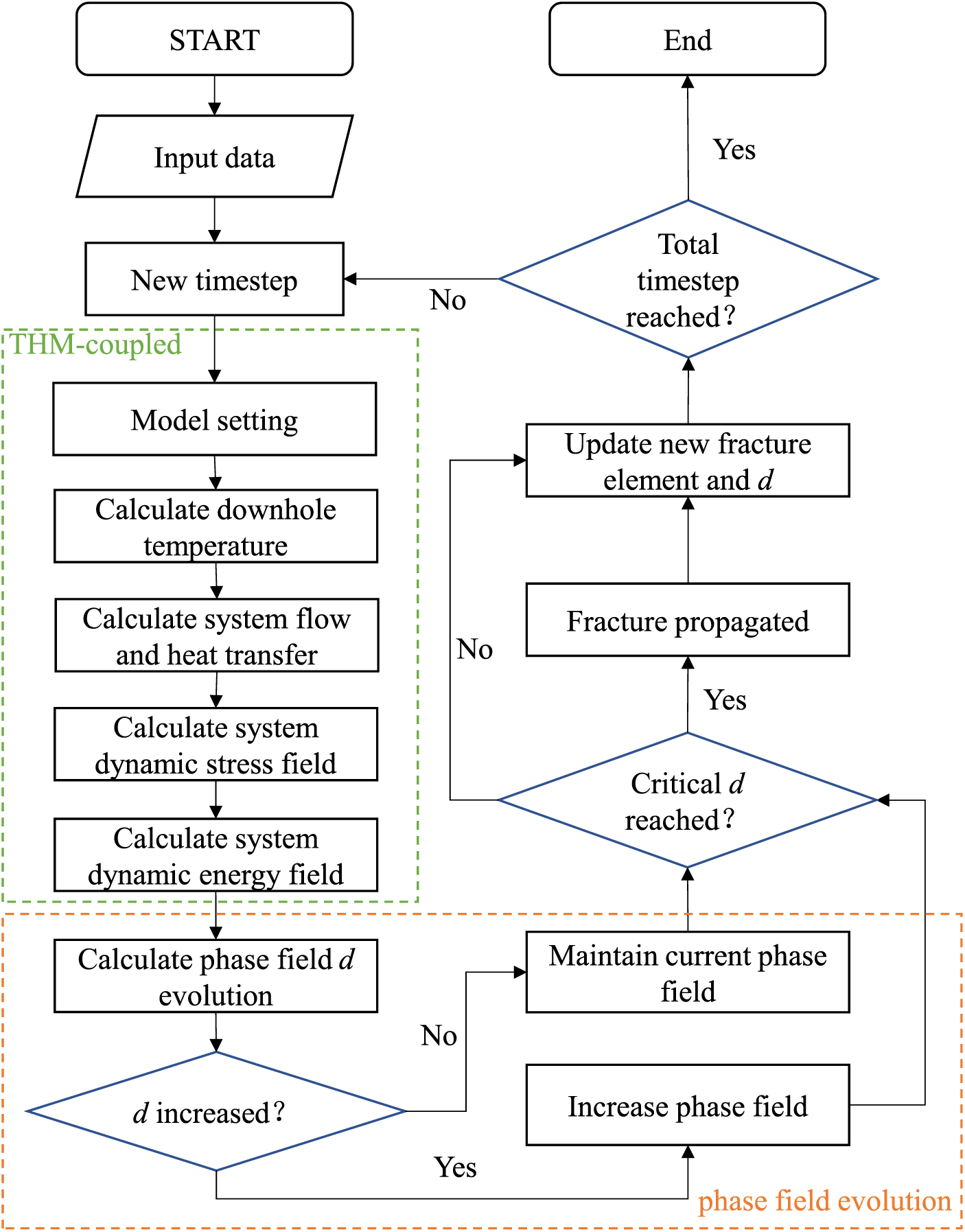
Figure 2: Flowchart of coupled field solution

We compared the previous phase field model to verify its accuracy in calculating fracture width. A homogeneous domain of 200 m × 200 m with an central injection point was established [28]. The Young’s modulus of the reservoir is set at 17 GPa, accompanied by a Poisson’s ratio of 0.2. The porosity and permeability of the reservoir are 0.003 mD and 20%, respectively. The critical energy release rate is set at 120 Pa·m and fluid viscosity is 0.4 mPa·s. As shown in Fig. 3, there is a good agreement between the analytical solution and the numerical solutions, with a small fraction of deviation less than 5%, so as to verify the presented model in this paper.

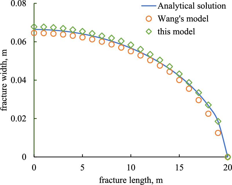
Figure 3: Validation of fracture width computation

3.2 Validation of THM-Coupled Stress Field

Due to the challenges in obtaining a suitable analytical solution for the multi physics problem [48], this paper employs the finite element software ABAQUS to simulate the stress distribution in a single fracture considering the influence of formation temperature and pore pressure. The application of the model in solving multi-physics coupled problems is verified by comparing the results simulated by the software with those derived from the model presented in this paper. As depicted in Fig. 4, a single fracture model consisting of a square plane strain model with dimensions of 0.05 m is established, featuring a crack of 0.02 m length and 0.001 m width at the center of the model. The external temperature boundary of the model is maintained at a constant temperature of 150°C, and the pressure boundary is defined as a closed boundary with rigid displacement conditions. In contrast, the temperature condition at the fracture within the model is set to a constant temperature of 40°C, with the fluid pressure maintained at 20 MPa and the displacement boundary is treated as a free boundary. The main model parameters are detailed in the Table 1. Additionally, two observation paths are included in the figure to quantitatively compare stress distribution and validate the stress computation accuracy of the proposed model.

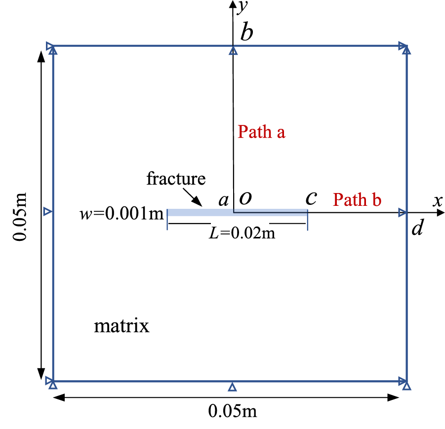
Figure 4: Diagram of THM-coupled stress field model (path a and path b in the figure are data observation paths)

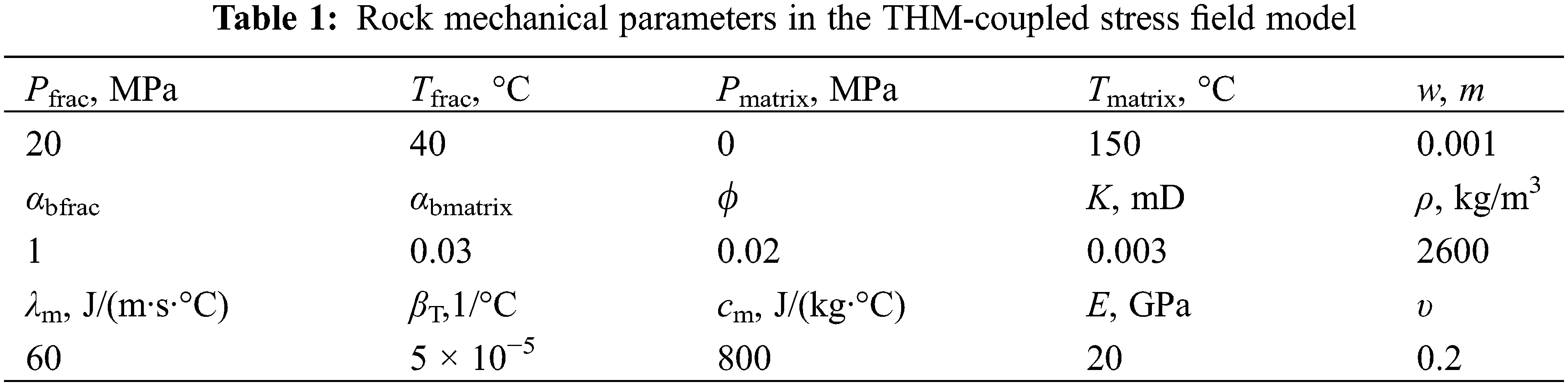
Fig. 5 illustrates the THM-coupled stress snapshots in the x and y directions as computed by the model presented in this study. It is evident that the stress distributions in different directions obtained from this research closely align with the ABAQUS results. Though a comparison of stress values along observation paths in both models depicted in the Fig. 6, it was determined that the average computation errors on path a and path b were 3.8% and 4.5%, respectively. Given that the principal stress of the elastic material is influenced by the rock displacement field, the comparative stress analysis serves to validate the accuracy of the model presented in this paper in computing fracture geometrical parameters within a THM-coupled environment.

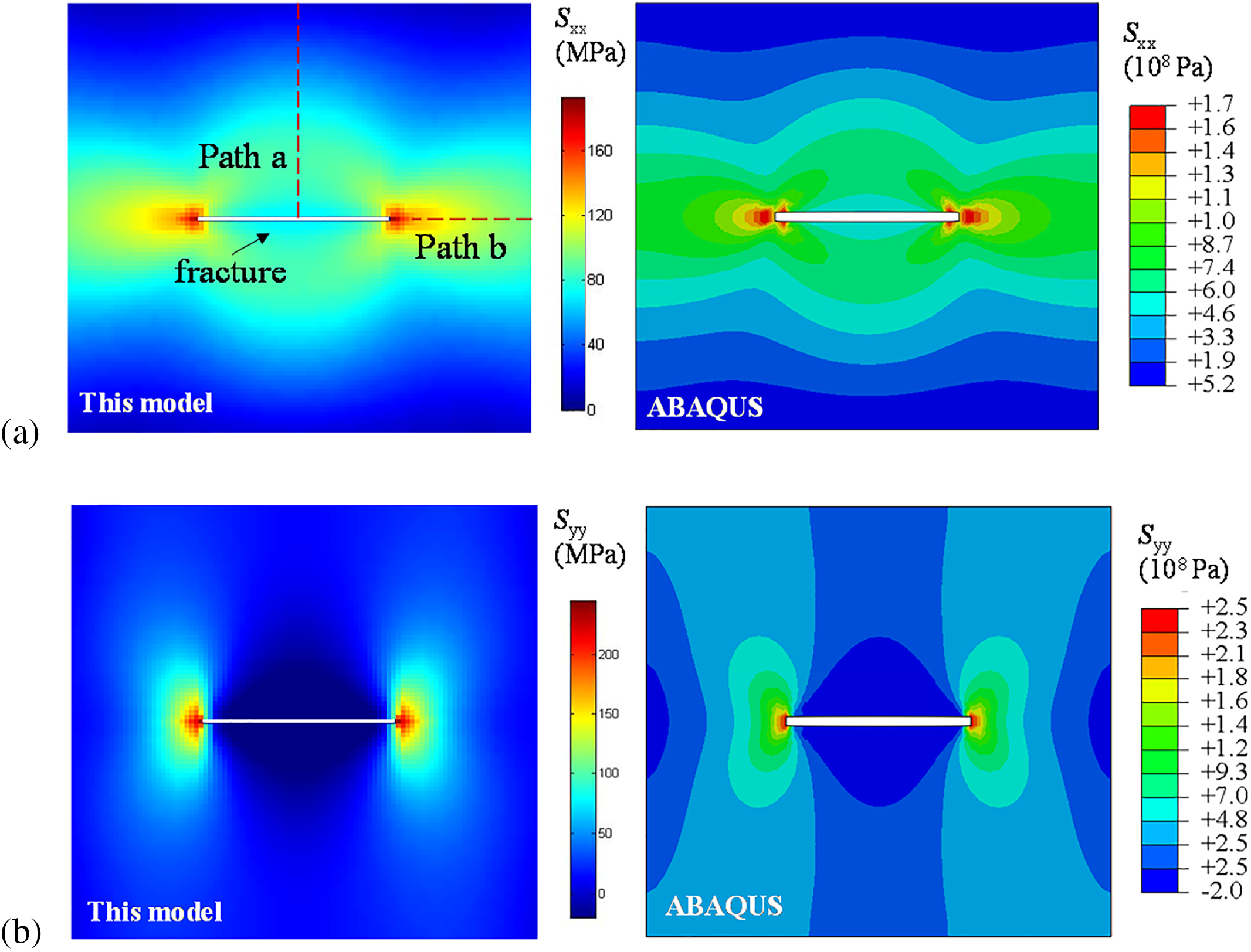
Figure 5: Stress distribution of the single fracture model simulated by the presented model and ABAQUS. (a) The principal stress SXX. Field simulated by the model presented in this paper (left) and the software (right). (b) The principal stress Syy. Field simulated by the model presented in this paper (left) and the software (right)

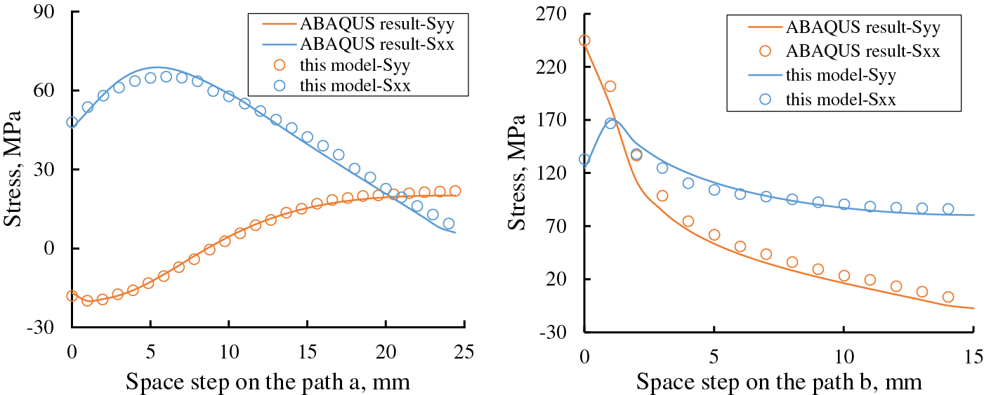
Figure 6: Comparison of the principal stress on observation path

3.3 Validation of Thermal Shock-Induced Fracture

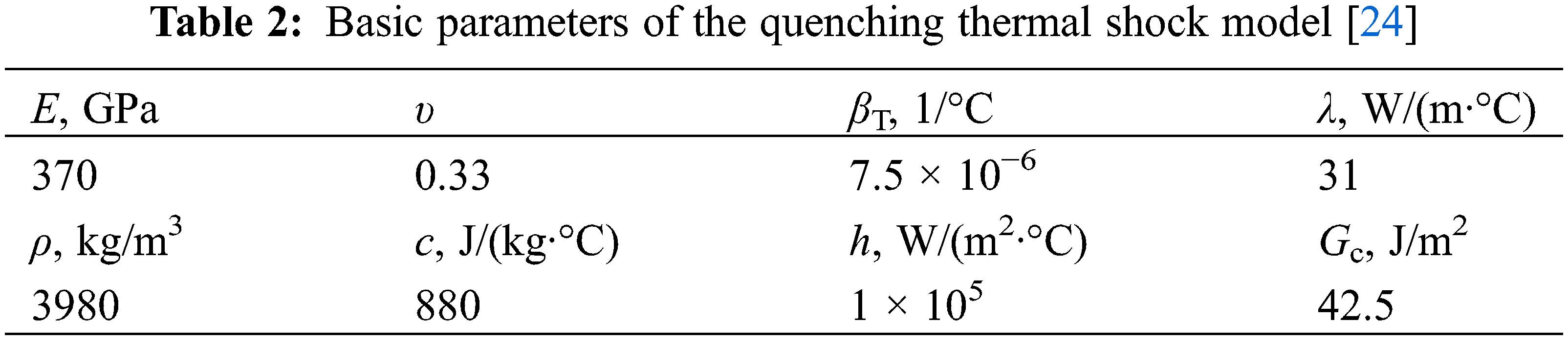
A comparative analysis is performed between the crack growth behaviors observed in ceramic slab quenching experiments and the simulated fracture morphology resulting from thermal shock using the THM-coupled fracture propagation model. Jiang et al. [49] subjected a ceramic slab to preheating followed by rapid cooling in a water bath, leading to the formation of numerous thermal cracks in the slab due to thermal shock. In this study, a two-dimensional plain strain model with dimensions of 25 mm in length and 10 mm in width is utilized for the quenching simulation model. The upper, lower, and right boundaries of the model are defined as convective heat transfer boundaries, while the left boundary is set as a thermal isolation boundary. The initial temperature of the model is 350°C, the cooling fluid temperature is 20°C, and the basic parameters of the model are shown in Table 2.

The thermal crack morphologies simulated in the proposed model closely match the thermal cracks observed in the quenched ceramic slab, as shown in Fig. 7. The comparison indicated that the numerical simulation accurately represents the behavior of thermal cracks, displaying parallel and periodic characteristic. Additionally, the simulation successfully replicates the phenomenon of ineffective propagation cracks due to stress interference, as evidenced by the red dashed box in Fig. 7. This analysis provides qualitative evidence of the proposed model’s capability and accuracy in simulating the thermal cracking process.

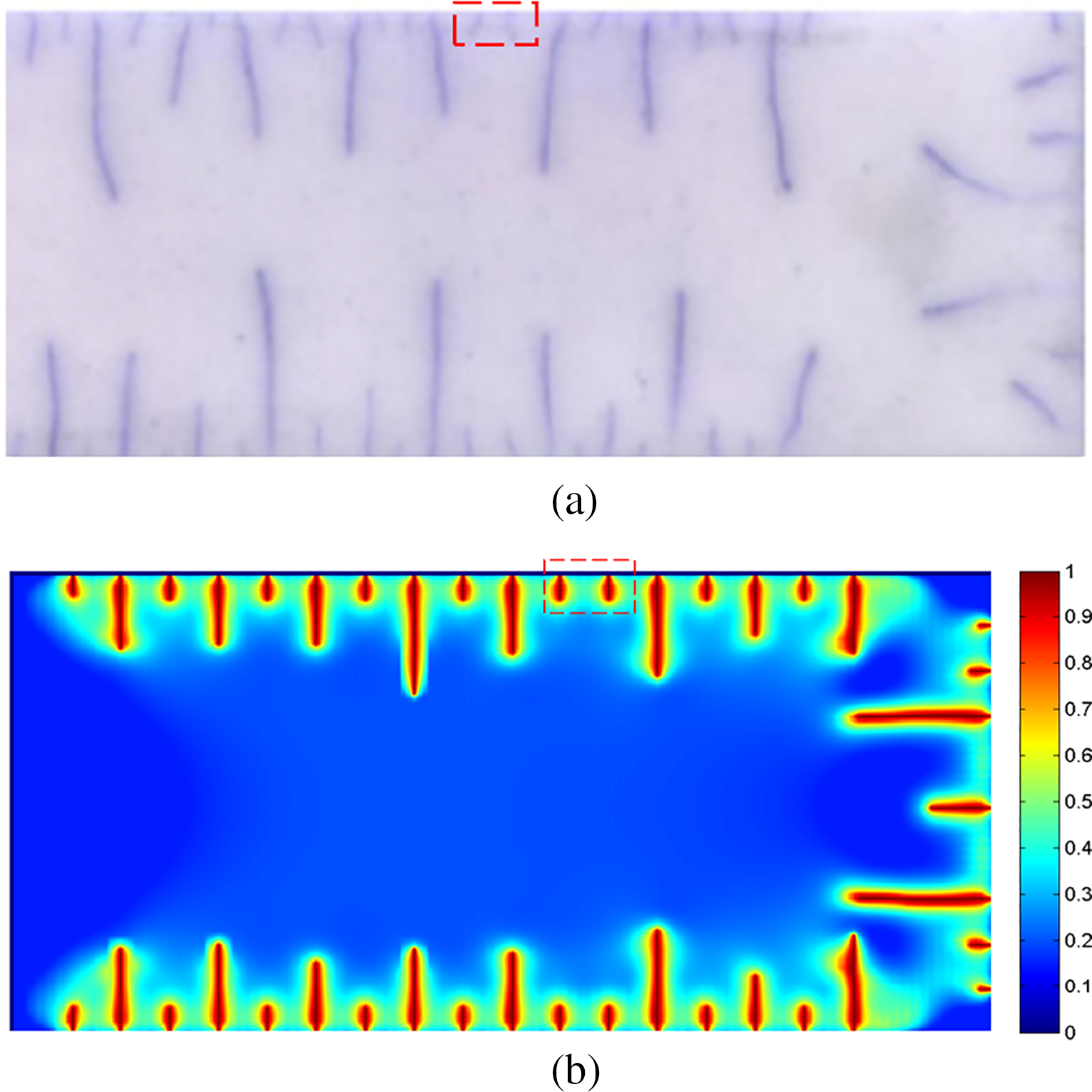
Figure 7: Comparison of thermal cracks generated in the quenching experiment [44] and the morphology of thermal shock fractures in the phase field modeling (In the phase field simulation result, the value 0 in the color bar indicates that the material is intact, the value 1 indicates that the material is broken, and other values indicate that the material is a damaged state). (a) Ineffective propagation cracks caused by thermal shock stress interference in the ceramic quenching test [44]. (b) Simulation of ineffective propagation cracks influenced by the thermal shock stress interference

4  Results and Discussion

4.1 Model Setting

Due to the low thermal conductivity of shale rock, the cooling impact of fracturing fluid primarily targets the fracture wall during the fracturing process. To investigate the mechanism of fracture propagation induced by thermal shock, a two-dimensional fracture propagation plain strain model measuring 0.1 m in length and 0.1 m in width was developed, and the grid size employed in this model is 5 × 10−4 m. In Fig. 8, an initial hydraulic fracture, measuring 0.01 m in length and 0.001 m in width, is positioned at the center of shale matrix. The x direction of the model represents the maximum horizontal principal stress σH, the y axis represents the minimum horizontal principal stress σh, and the fracture trend aligns with the direction of σH. The research focuses on the damage impact of thermal shock on shale rock, hence a constant pressure boundary with the fracture net pressure Pnet is set as the fluid pressure inside the fracture, while the initial fluid pressure in the porous matrix is defined as Pp. The model’s outer boundaries for pressure, temperature, and stress are specified as the closed boundary, fixed displacement boundary, and thermal isolation boundary, respectively. The data observation paths, denoted by three yellow dotted lines, are included in the model to facilitate quantitative comparison and analysis of simulation results. Positive directions are defined as right along the x-axis and down along the y-axis.

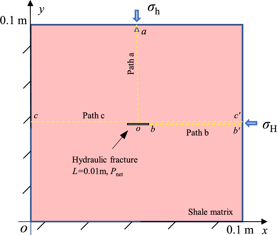
Figure 8: Diagram of single fracture propagation model

The fracture convective heat transfer parameters in the model are adopted from Tang et al. [23], with all parameters set accordingly.

4.2 Thermal Shock Damage Analysis with Dynamic Fluid Temperature

The study initially examines the thermal shock damage effect near the fracture by comparing the induced stress and phase-field distributions between cases considering thermal shock considering the thermal shock effect (TS) and normal cases (NM). In both models, the fracture net fluid pressure is set to 6 MPa, and the fluid temperature inside the fracture in the TS case is maintained at 40°C to minimize external influences. Fig. 9 illustrates the displacement, induced stress, and phase field distribution in both cases at t = 100 s. In the NM case, the rock mass at the fracture wall moves outward in the x and y directions due to the load of the fracture fluid pressure. While in the TS case, as shown in Fig. 10, the temperature decreases on the fracture wall and tip are 96°C and 65°C after water cooling. The cooled rock shrinkage displacement is constrained by the high-temperature rocks, leading to tensile stress formation in the matrix near the fracture. Due to the stress concentration effect, the induced stress and damage distribution around the fracture in the TS case to be much larger than that in the NM case.

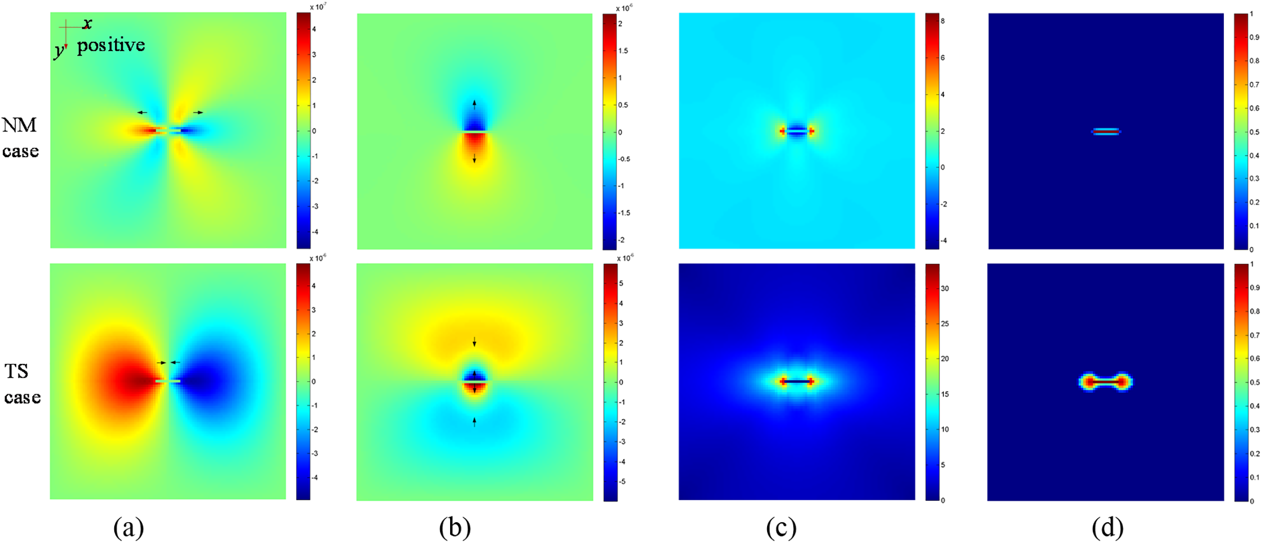
Figure 9: Snapshots of distribution of the displacement, the induced stress, and the phase field in the NM case and TS case after 100 s cooling. (a) Displacement in the x direction. (b) Displacement in the y direction. (c) Distribution of induce stress. (d) Distribution of phase field

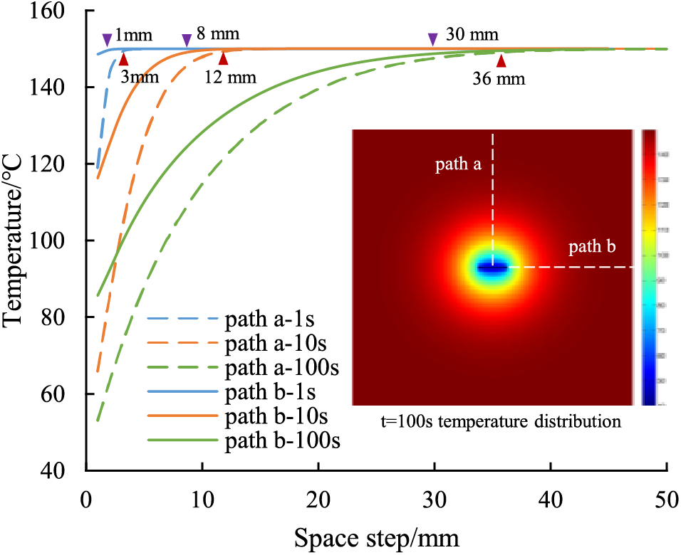
Figure 10: Curves of temperature distribution on data paths in the TS case with different cooling times

The snapshot in the figure depicts the temperature distribution of the TS case at t = 100 s, the white dashed lines are marked to show the position of data observation paths, and the solid triangle on the curves marks the effect cooling range.

Fig. 11 presents a quantitative comparison of displacement and induced stress distribution in both cases along observation paths. The results show that thermal shock significantly increased the displacement of the rock mass surrounding the fracture, consequently enhancing the induced stress near the fracture. In comparison to the NM case, the average stress along both paths in the TS case increased by 4.6 and 7.1 MPa, respectively. The induced stress at the fracture wall transitioned from a compressive stress of −4.1 MPa to a tensile stress of 8.7 MPa. The significant contraction of rock at the fracture tip led to a more concentrated stress at the fracture tip. Furthermore, as depicted in Fig. 9, the tensile stress area and rock phase field near the fracture were both intensified caused by the thermal shock effect. The damaged area transformed from a small stripe in the NM case to a dumbbell shape in the TS case, indicating that thermal shock effectively weakens the rock strength near the fracture, thereby promoting fracture initiation and extension in deep shale.

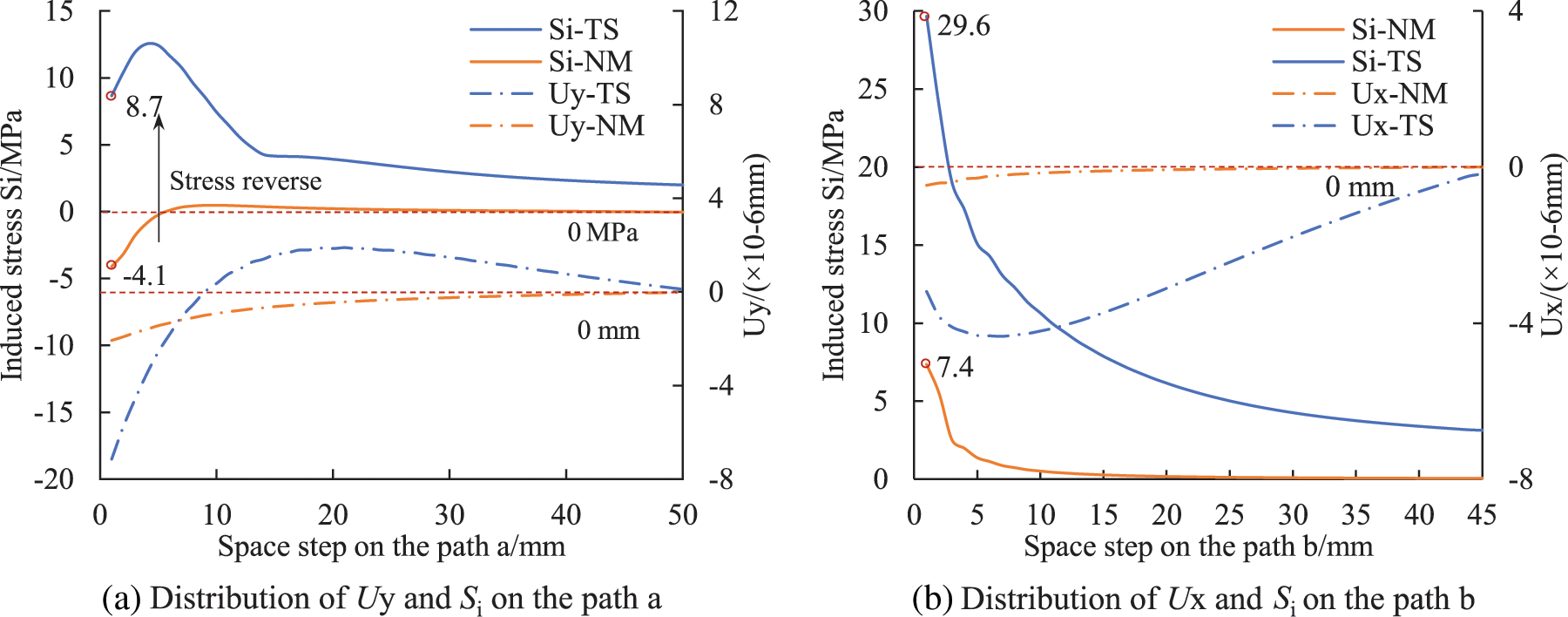
Figure 11: The displacement in both axial directions (Ux, Uy) and the induced stress (Si) distribution in NM and TS cases on the data observation paths. (a) Distribution of Uy and Si on the path a. (b) Distribution of Ux and Si on the path b

The fluid temperature inside the fracture changed dynamically throughout the injection process due to the wellbore heating effect. In Fig. 12, variations in rock temperature at the fracture wall and tip are shown under static temperature (ST) and dynamic temperature (DT) conditions. In the ST case, where the fluid temperature remained constant at 40°C, the temperature curves initially dropped sharply with the first 25 s due to the significant initial difference between the fluid and matrix temperatures. As the contact temperature difference decreased, the curves eventually stabilized at 50.9°C and 78.6°C. On the other hand, when considering the wellbore heating effect, the dynamic bottom-hole temperature led to a gradual decline in the temperature curves in the TS case, resulting in final temperatures of 81.9°C and 104.5°C, respectively. The difference in temperature decrease trend suggests that the fracture fluid temperature plays a significant role in determining the temperature distribution near the fracture. Therefore, the model hypothesized that relying solely on static fluid temperature may lead to an overestimation of the cooling efficiency of the fracturing fluid.

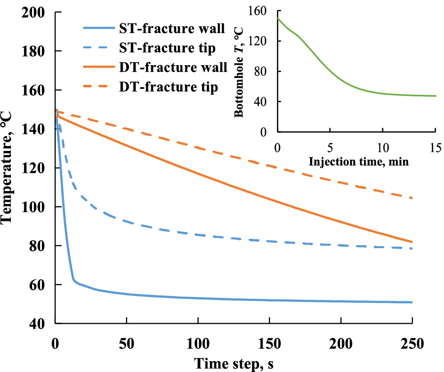
Figure 12: Evolution of rock temperature at fracture wall and tip under different temperature conditions

The image in the upper right corner of Fig. 12 shows the dynamic bottom-hole temperature, and the abbreviation ST and DT in the legend represent the static and dynamic temperature conditions.

Thermal stress is influenced by the temperature gradient in the matrix. Fig. 13 illustrates the variation of induced stress at observation points under different temperature conditions. In the case of a significant initial temperature difference between the original fluid and fracture wall, stress curves in the ST case exhibit a rapid initial increase. For instance, stress at the fracture wall escalates from −2.8 to 9.4 MPa within the first 15 s. As the fracture temperature field gradually approached a steady state under static temperature conditions, the stress curves exhibited a slower rate of change with increasing cooling times. Conversely, in the DT case with a lower contact temperature difference, stress curves remained lower compared to the ST case. The thermal shock caused by the temperature variation enhances tensile stress near the fracture, particularly at the fracture tip, when contrasted with the steady stress distribution in the NM case. The disparity in cooling efficiency between the two temperature conditions results in significant differences in induced stress levels at the fracture wall and tip, reaching up to 3.3 and 12.2 MPa, respectively.

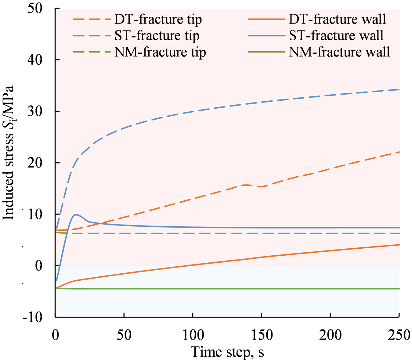
Figure 13: Evolution of the induced stress of the matrix at fracture wall and fracture tip under different fracture fluid temperature conditions (the red area indicates the tensile stress with a stress value beyond 0 MPa, the blue area indicates the compressive stress with a stress value below 0 MPa)

The difference in thermal stress between the two temperature cases resulted in distinct rock damage characteristics. In Fig. 14, the dynamic evolution of the phase field at observation points and damage areas is presented for both cases. Under high tensile stress loads, the phase field of the rock at the fracture tip in the ST case quickly increased to 0.8 initially and then gradually approached 0.95. On the other hand, in the DT case, the phase field curve originally increased slowly but then sharply rose when the tensile energy reached a critical value at 145 s. This sharp increase in damage even caused a decline in the stress curve at that time step, as depicted in Fig. 11 for the DT case. At the fracture wall, the phase field curves in both cases increased rapidly and reached a steady state due to the resistance of fluid compression stress. However, the phase field values at the fracture wall and tip in the DT case were 25.6% and 20% lower than those of the ST case, respectively. By defining elements with a phase field value above 0.5 as damaged, it was observed that the damaged area in the ST and DT cases were 8 and 74 mm2, respectively. These findings indicate that the severity of thermal shock damage is influenced by the rock cooling degree, with a significantly higher impact on the fracture tip compared to the fracture wall. Overall, assuming static fracture fluid temperatures in fracture propagation simulations may exaggerate rock thermal shock damage severity, suggesting that considering dynamic downhole temperature is more rational in THM-coupled fracture propagation computations.

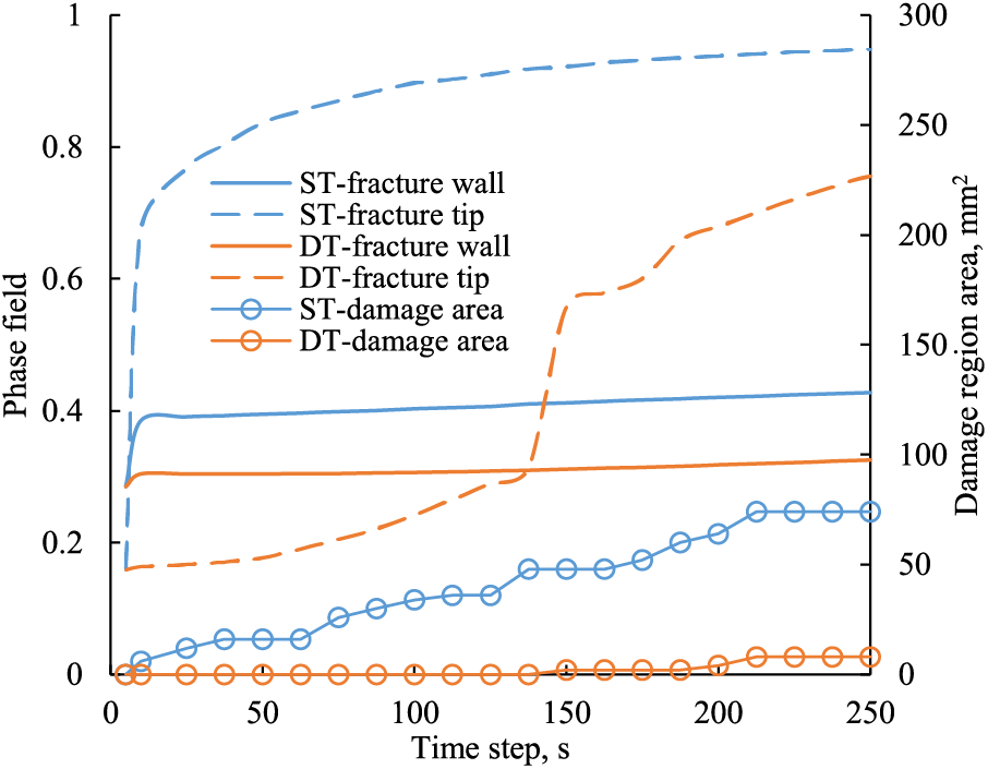
Figure 14: Evolution of phase field and damaged area of the matrix at fracture wall and fracture tip under different fracture fluid temperature conditions

4.3 Thermal Shock Damage Analysis with Different Fracture Net Pressure

Fig. 15 illustrates a comparison of the induced stress distribution induced in NM and TS cases under different fracture net pressure. Images of both cases were captured simultaneously for accurate comparison. The compressive stress on the fracture wall in cases without thermal shock increased with higher fracture net pressure, leading to stress concentration at the fracture tip but no initiation of fractures. In contrast, thermal shock intensified tensile stress around the fracture, enabling fracture initiation. Moreover, unlike previous studies showing single-point failure at the fracture tip, thermal shock induced multiple initiation and micro cracks, indicating thermal shock increased severity and range of rock damage at the fracture tip. For instance, Fig. 16 shows an intensified tensile stress region near the fracture tip with an average stress exceeding 25 MPa during the initiation moment in the Pnet = 15 MPa case. When the rock’s tensile energy accumulation reached critical failure energy at the second time step, the original fracture tip ruptured. As a result of the significant damage from thermal shock, rocks at the core of the tensile stress region all fractured and formed multiple failures at the fracture tip in Step 3, causing the fracture to extend further. The stress release due to rock damage created an elliptical damaged area between the fracture tip and the high tensile stress region, as depicted in the image of Step 4, resulting in an arc-shaped high stress region. Additionally, as the damage continued, these micro failures gradually developed into branch fractures during the propagation of the main fracture.

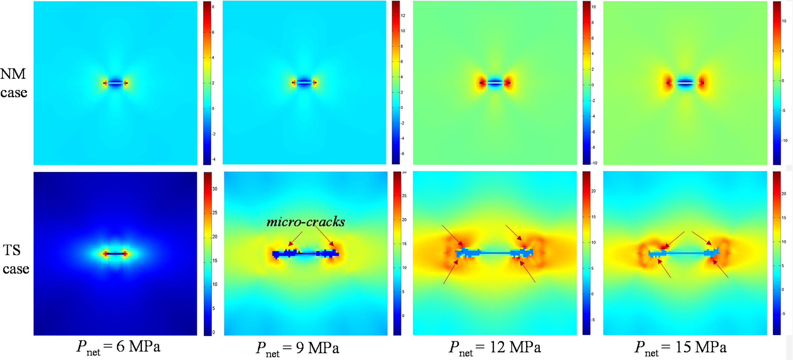
Figure 15: Snapshots of fracture initiation induced stress field in NM and TS cases with different fracture net pressure conditions

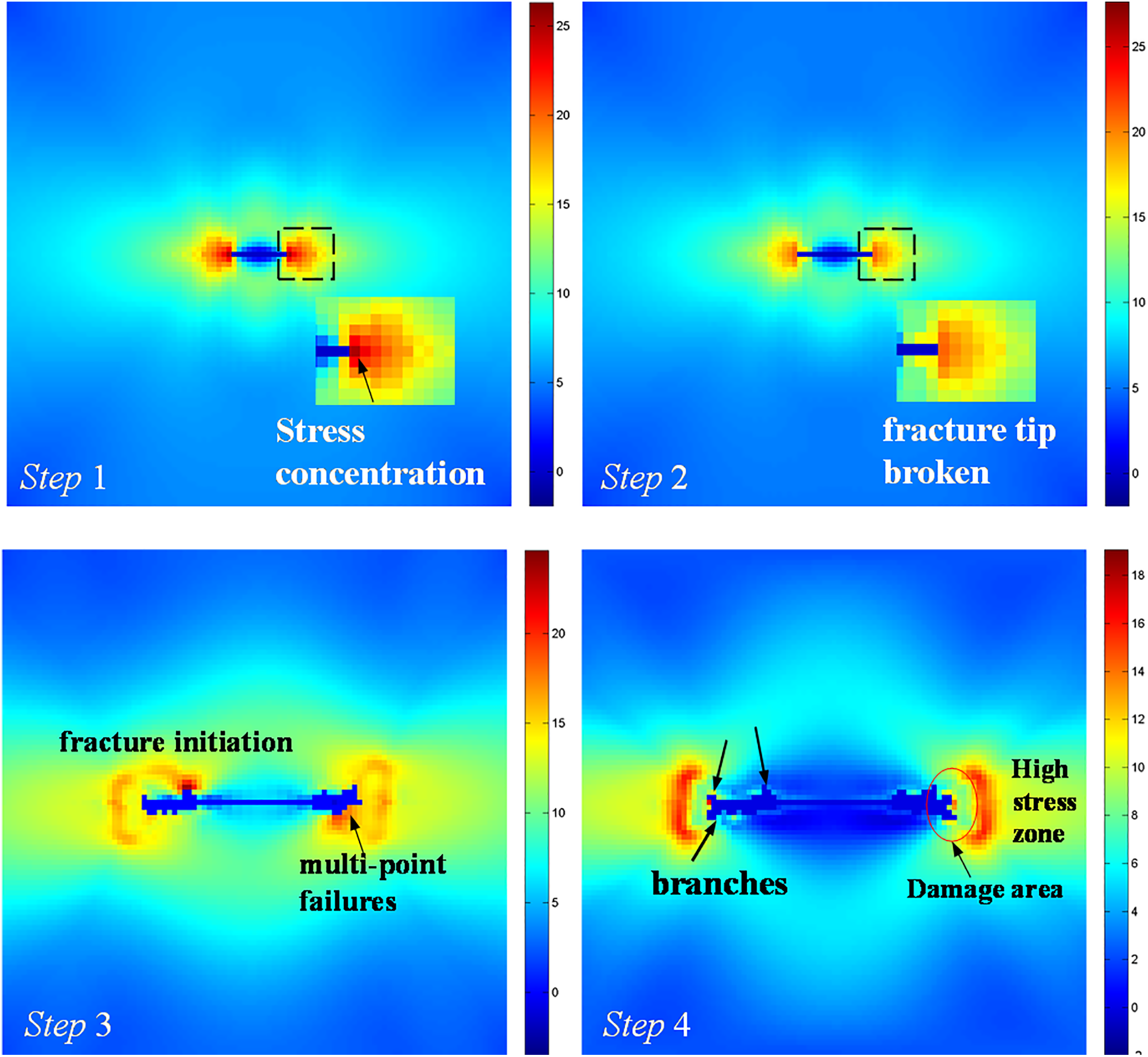
Figure 16: Snapshots of induced stress field at the fracture initiation moment of 15 MPa fracture net pressure case considering thermal shock effects

Fig. 17 quantitatively examines the impact of thermal shock on the tensile energy of rock at the fracture tip. The study reveals that the energy density curve in the NM case remains stable, with the energy density value increasing as the fracture net pressure rises. This phenomenon occurs because the internal stress of the matrix near the fracture reaches equilibrium under constant fluid pressure loads. The stress balance is disrupted only when the fluid pressure surpasses the critical failure condition. However, due to thermal stress accumulation during the cooling process, the energy density curve in the TS cases gradually increases until reaching the critical failure condition, at which point the curve sharply declines, indicating complete rock fracture. With an increase in fracture fluid pressure, there is a greater accumulation of tensile energy density at the fracture tip, resulting in earlier fracture initiation. Additionally, as depicted in Fig. 15, the damaged area at the fracture tip propagates with higher fracture fluid pressure, necessitating higher tensile energy for fracture initiation in cases of elevated net pressure. Overall, these comparative analyses suggest that thermal shock can supply additional tensile energy at the fracture tip, facilitating fracture initiation in deep shale. The multi-point mode failure induced by thermal shock may result in branch fractures forming after fracture initiation.

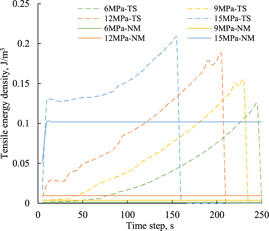
Figure 17: Variation of the tensile energy density of the rock at the fracture tip in NM and TS cases with different fracture fluid net pressure

4.4 Thermal Shock Damage Analysis on Bedding Planes

This section investigates the influence of thermal shock on fractures interacting with bedding planes formed in deep shale. As shown in Fig. 18, four horizontal beddings (B1 to B4), each with a length of 0.16 m, were incorporated to the previously established sigle fracture model. The beddings have a spacing of 20 mm, and the model size is increased to 0.15 m × 0.2 m. Based on experimental data from Heng et al. [50], the Young’s modulus, Poisson’s ratio and fracture toughness of bedding planes are reported as 15,000 MPa, 0.3, and 0.5 MPa/m0.5, respectively. Assuming the bedding planes are initially cemented, the phase field of the bedding planes is set to 0, while other parameters can be referenced in Table 3.

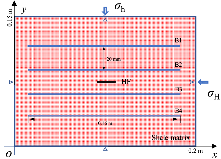
Figure 18: Diagram of single fracture propagation model with multiple natural fractures

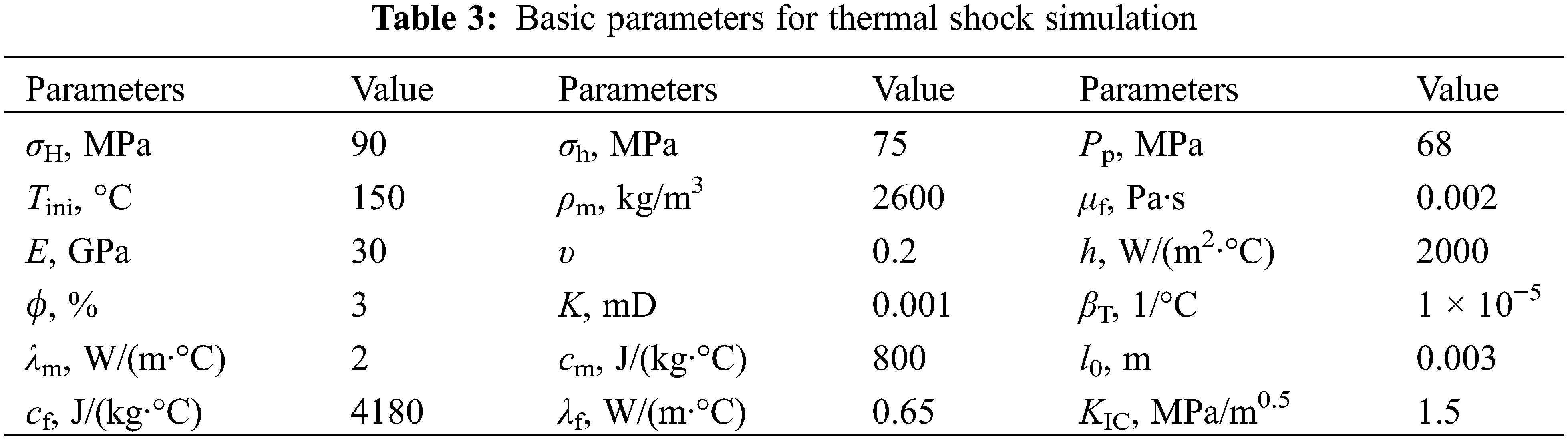
Fig. 19 illustrates the dynamic fracture interaction behaviors in deep shale with bedding planes under a fracture net pressure of 15 MPa. Initially, the fracture tip experienced damage due to stress concentration, while the internal stress of the matrix reached equilibrium. As the temperature of the fracture wall gradually decreased over time, the damaged value and area of the rock at the fracture tip increased. Additionally, the bedding planes surrounding the fracture were damaged by thermal shock. When the temperature dropped to t = 164 s, the rocks at the fracture tip of both wings were destroyed, leading to fracture initiation. Approximately half of the bedding planes were damaged with an average phase-field value of 0.95. As the fracture extended, multiple failures occurred at the fracture wall, particularly at weak bedding planes near the damaged region of the fracture tip. When the cooling time reached 165 s, the left wing of the fracture diverted to the B2 bedding plane, while the right-wing turned to B3.

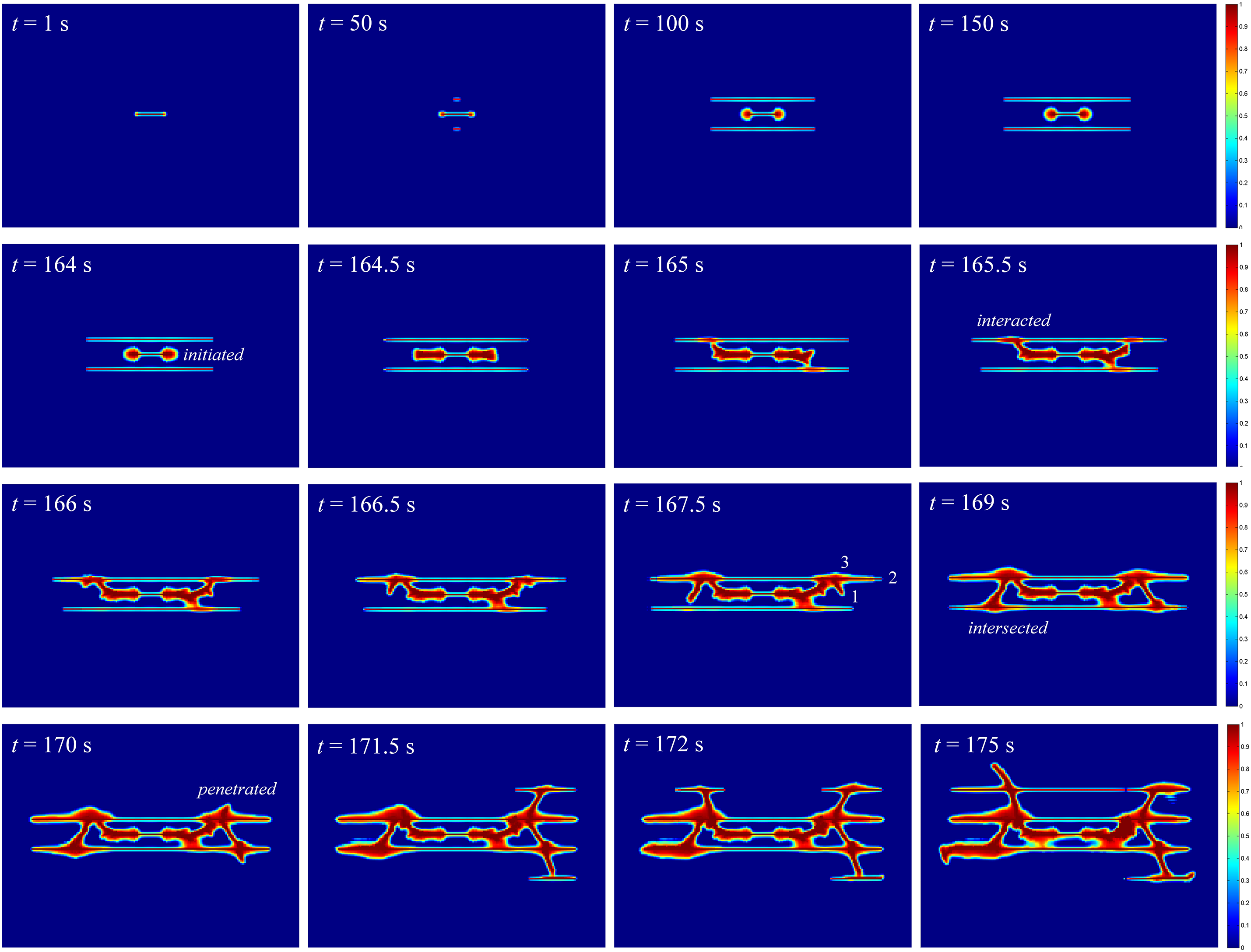
Figure 19: Snapshots of phase field distribution of propagated fractures in deep shale with bedding planes

As depicted in Fig. 20, the induced stress distribution analysis reveals that the local stress field was significantly influenced by the partially activated bedding planes at t = 164.5 s. This led to the diversion of two wings of the propagating fracture, triggering the activation of the bedding planes. Upon intersecting with the bedding plane, branch fractures were formed on both wings of the fracture due to thermal shock. As shown in the figure of t = 167.5 s, three branches emerged on the right wing of the fracture. Branch 1 propagated towards the B3 bedding plane, Branch 2 extended along the B2 bedding plane, and Branch 3 pierced through the bedding plane towards the B1 plane. Similarly, on the left wing of the fracture, three branches were observed after interacting with the B2 plane, with an upward propagating crack even penetrating the B1 plane. Above analysis reveals that water cooling thermal shock can activate natural fractures surrounding hydraulic fractures. Thermal shock damage to natural fractures alters the induced stress field, causing hydraulic fractures to divert and interact with natural fractures. Moreover, thermal shock enhances the penetration ability of hydraulic fracture tips, enabling hydraulic fractures to penetrate natural fractures and activate additional natural fractures, resulting in the formation of complex fracture patterns.

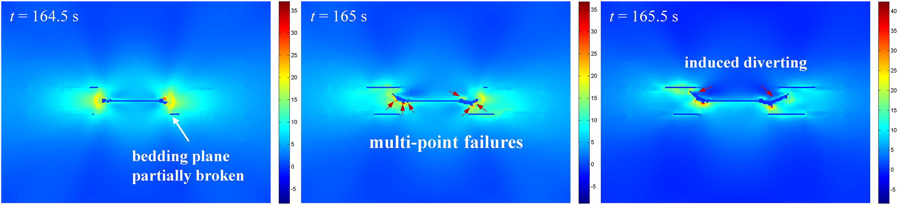
Figure 20: Induced stress distribution of thermal shock-induced fracture at the fracture initiation moment

Fig. 21 records the initiation morphologies of thermal shock induced fractures in bedding shale under different fracture net pressures (10, 15, and 20 MPa) to analyze the impact of fracture net pressure on thermal shock induced fracture patterns. The fracture initiation and propagation towards the model boundary occurred within 0.5 s when the fracture net pressure reached 20 MPa, resulting in partial damage of bedding near the fracture due to stress concentration at the fracture tip. Conversely, fracture initiation took nearly 200 s in the case of Pnet = 10 MPa, and the initiated fractures diverted and propagated along the bedding planes. The phenomenon indicates that it is difficult for cracks to initiate under the current pressure condition, fracture initiation is actually a process of gradual accumulation of thermal shock damage. In the case of Pnet = 15 MPa, cracks with penetrating ability were enhanced by the fluid pressure and thermal shock effects, leading to the formation of a fracture network. These findings suggest that fracture net pressure remains the primary driver of fracture propagation in shale rock due to its lower fluid cooling efficiency. High fracture net pressures can initiate rapidly and propagate without being affected by damaged bedding planes, as illustrated in Fig. 21c. In cases where fractures fail to initiate due to lower net pressure, thermal shock-induced stress can damage the matrix and bedding planes near the fracture, facilitating fracture initiation. Additionally, the thermal shock effect can affect fracture propagation behavior by altering the local stress distribution at the fracture tip. However, due to limitations in fluid cooling efficiency, it takes longer for thermal shock to accumulate enough tensile strain energy to fracture the formation. Consequently, thermal shock-induced fractures exhibit lower penetrating ability compared to fractures under high fracture net pressure conditions.

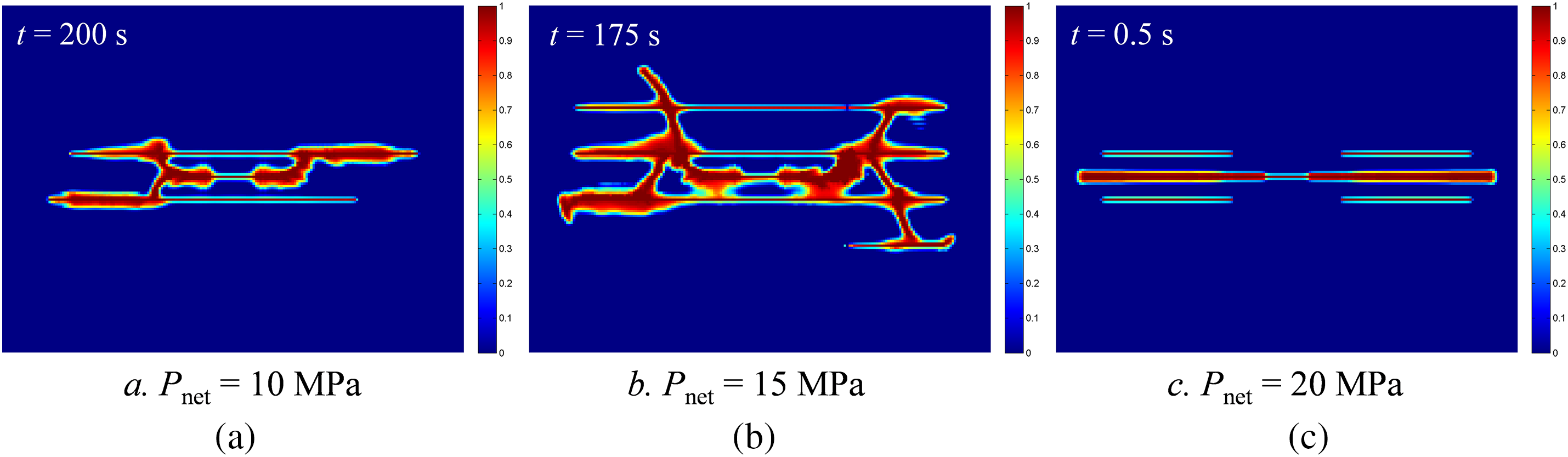
Figure 21: Snapshots of initiation morphologies of thermal shock-induced fractures under different fracture net pressure (a) Pnet = 10 MPa (b) Pnet = 15 MPa (c) Pnet = 20 MPa

5  Conclusions

This paper presents a THM-coupled fracture propagation model based on the phase field method. The model’s application was validated by comparing stress distribution and quenching fracture morphologies with software simulation results quantitatively and ceramic quenching test results qualitatively. The study investigates thermal shock-induced fracture propagation behaviors in deep shale and draws several conclusions:

(1)   The cooling of cracks creates a temperature decrease gradient with the rock mass, leading to a discrepancy in thermal strain levels in the rock. This variation results in thermal tensile stress, significantly enhancing the tensile strain energy in the surrounding rock mass, deteriorating rock strength and facilitating initiation and propagation of cracks.

(2)   The severity of thermal shock damage is directly influenced by fluid cooling efficiency. Applying a constant fracture temperature condition may result in overestimation errors, whereas considering wellbore temperature variation is more appropriate in THM-coupled fracture propagation computation.

(3)   Thermal shock introduces additional tensile strain energy, resulting in the formation of an arc-shaped high-stress region and an elliptical damaged area at fracture tip. This leads to a multi-point failure mode in the crack, with branch fractures forming due to alterations in the induced stress field.

(4)   Thermal shock can activate pre-existing fractures near hydraulic fractures and improve the penetration capability of hydraulic fractures. This enables hydraulic fractures to penetrate natural fractures and induce the activation of more natural fractures, leading to the development of fracture networks.

Acknowledgement: This paper is prepared under the auspices of the State Key Laboratory of Oil and Gas Reservoir Geology and Exploitation of Southwest Petroleum University and CNOOC Research Institute Ltd.

Funding Statement: This paper is funded by the CNOOC Science and Technology Project (KJGG2022-0701) and the National Natural Science Foundation of China (51904258, 51874250).

Author Contributions: Zhuang Liu: Conceptualization, Methodology, Writing—review & editing, Project administration; Tingen Fan: Methodology, Formal analysis, Writing; Qianli Lu: Conceptualization, Methodology, Supervision, Resources; Jianchun Guo: Validation, Formal analysis, Funding acquisition; Renfeng Yang: Validation, Formal analysis; Haifeng Wang: Formal analysis. All authors reviewed the results and approved the final version of the manuscript.

Availability of Data and Materials: The datasets generated and/or analyzed during the current study are available from the corresponding author on reasonable request.

Ethics Approval: Not applicable.

Conflicts of Interest: The authors declare no conflicts of interest to report regarding the present study.

References

1. Zhang F, Wu J, Huang H, Wang X, Luo H, Yue W, et al. Technological parameter optimization for improving the complexity of hydraulic fractures in deep shale reservoirs. Nat Gas Ind. 2021;41(1):125–35. [Google Scholar]

2. Ma X, Wang H, Zhao Q, Liu Y, Zhou S, Hu Z, et al. Extreme utilization development of deep shale gas in South Sichuan Basin, SW China. Pet Explor Dev. 2020;49(6):1190–7. [Google Scholar]

3. Yavuz H, Demirdag S, Caran S. Thermal effect on the physical properties of carbonate rocks. Int J Rock Mech Min Sciences. 2010;47(1):94–103. doi:10.1016/j.ijrmms.2009.09.014. [Google Scholar] [CrossRef]

4. Khalid E, Hossein E, Mahdi R. Investigating effects of thermal shock technique on unconventional reservoir rock mechanical properties. In: The 53rd US Rock Mechanics/Geomechanics Symposium, 2019 Jun 23; New York, NY, USA. [Google Scholar]

5. Song H, Shi H, Chen Z, Li G, Ji R, Chen H. Numerical study on impact energy transfer and rock damage mechanism in percussive drilling based on high temperature hard rocks. Geothermics. 2021;96(3):102215. doi:10.1016/j.geothermics.2021.102215. [Google Scholar] [CrossRef]

6. Enayatpour S, van Oort E, Patzek T. Thermal cooling to improve hydraulic fracturing efficiency and hydrocarbon production in shales. J Nat Gas Sci Eng. 2019;62(5):184–201. doi:10.1016/j.jngse.2018.12.008. [Google Scholar] [CrossRef]

7. Huang Z, Zhang S, Yang R, Wu X, Li R, Zhang H, et al. A review of liquid nitrogen fracturing technology. Fuel. 2020;266(30):117040. doi:10.1016/j.fuel.2020.117040. [Google Scholar] [CrossRef]

8. Zhang H, Huang Z, Zhang S, Yang Z, Mclennan D. Improving heat extraction performance of an enhanced geothermal system utilizing cryogenic fracturing. Geothermics. 2020;85(3):101816. doi:10.1016/j.geothermics.2020.101816. [Google Scholar] [CrossRef]

9. Jiang X, Chen M, Li Q, Liang L, Zhong Z, Yu B, et al. Study on the feasibility of the heat treatment after shale gas reservoir hydration fracturing. Energy. 2022;254(2):124422. doi:10.1016/j.energy.2022.124422. [Google Scholar] [CrossRef]

10. Cai C, Li G, Huang Z, Shen Z, Tian S, Wei J. Experimental study of the effect of liquid nitrogen cooling on rock pore structure. J Nat Gas Sci Engineering. 2014;21(3–4):507–17. doi:10.1016/j.jngse.2014.08.026. [Google Scholar] [CrossRef]

11. Xi B, Wu Y, Wang S, Xiong G, Zhao Y. Evolution of mechanical properties of granite under thermal shock in water with different cooling temperatures. Rock Soil Mech. 2020;41:83–94. [Google Scholar]

12. Memon KR, Ali M, Awan FUR, Mahesar AA, Abbasi GR, Mohanty US, et al. Influence of cryogenic liquid nitrogen cooling and thermal shocks on petro-physical and morphological characteristics of Eagle Ford shale. J Nat Gas Sci Eng. 2021;96:104313. doi:10.1016/j.jngse.2021.104313. [Google Scholar] [CrossRef]

13. Kang Y, Yang D, You L, Li X, Bai J, Shao J, et al. Experimental evaluation method for permeability changes of organic-rich shales by high-temperature thermal stimulation. J Nat Gas Geoscience. 2021;6:145–55. doi:10.1016/j.jnggs.2021.07.001. [Google Scholar] [CrossRef]

14. Vikram V, Mohd R, Bankim M, Pradhan S, Singh T. Temperature effect on the mechanical behavior of shale: implication for shale gas production. Geosyst Geoenviron. 2022;1:100078. doi:10.1016/j.geogeo.2022.100078. [Google Scholar] [CrossRef]

15. Altawati F, Emadi H. Effects of cyclic cryogenic treatment on rock physical and mechanical properties of Eagle Ford shale samples—An experimental study. J Nat Gas Sci Eng. 2020;88:103772. [Google Scholar]

16. Altawati F, Emadi H, Pathak S. Improving oil recovery of Eagle Ford shale samples using cryogenic and cyclic gas injection methods—An experimental study. Fuel. 2021;302:121170. doi:10.1016/j.fuel.2021.121170. [Google Scholar] [CrossRef]

17. Wu Y, Tao J, Wang J, Zhang Y, Peng S. Experimental investigation of shale breakdown pressure under liquid nitrogen pre-conditioning before nitrogen fracturing. Int J Min Sci Technology. 2021;31:611–20. doi:10.1016/j.ijmst.2021.05.006. [Google Scholar] [CrossRef]

18. Guo T, Zhang Y, Shen L, Liu X, Duan W, Liao H, et al. Numerical study on the law of fracture propagation in supercritical carbon dioxide fracturing. J Petrol Sci Eng. 2022;208:109369. doi:10.1016/j.petrol.2021.109369. [Google Scholar] [CrossRef]

19. Li D, Li P, Li W, Zhou K. Three-dimensional phase-field modeling of temperature-dependent thermal shock-induced fracture in ceramic materials. Eng Fract Mechani. 2022;268:108444. doi:10.1016/j.engfracmech.2022.108444. [Google Scholar] [CrossRef]

20. Lu Q, Guo J, Liu Z, Ren Y, Wang X, Guan B, et al. Investigation of thermal induced damage of deep shale considering in-situ thermal shock effects. Geoenergy Sci Eng. 2023;222:211439. doi:10.1016/j.geoen.2023.211439. [Google Scholar] [CrossRef]

21. Yao B, Wang L, Yin X, Wu Y. Numerical modeling of cryogenic fracturing process on laboratory-scale Niobrara shale samples. J Nat Gas Sci Eng. 2017;48:169–77. doi:10.1016/j.jngse.2016.10.041. [Google Scholar] [CrossRef]

22. Sun L, Liu Q, Grasselli G, Tang X. Simulation of thermal cracking in anisotropic shale formations using the combined finite-discrete element method. Comput Geotech. 2020;117(6):103237. doi:10.1016/j.compgeo.2019.103237. [Google Scholar] [CrossRef]

23. Tang S, Wang J, Chen P. Theoretical and numerical studies of cryogenic fracturing induced by thermal shock for reservoir stimulation. Int J Rock Mech Min. 2020;125:104160. doi:10.1016/j.ijrmms.2019.104160. [Google Scholar] [CrossRef]

24. Liu J, Liang X, Xue Y, Yao K, Fu Y. Numerical evaluation on multiphase flow and heat transfer during thermal stimulation enhanced shale gas recovery. Appl Therm. 2020a;178:115554. doi:10.1016/j.applthermaleng.2020.115554. [Google Scholar] [CrossRef]

25. Guo Y, Li X, Huang L. Changes in thermophysical and thermomechanical properties of thermally treated anisotropic shale after water cooling. Fuel. 2022;327(11):125241. doi:10.1016/j.fuel.2022.125241. [Google Scholar] [CrossRef]

26. Li X, You L, Kang Y, Liu J, Chen M, Zeng T, et al. Investigation on the thermal cracking of shale under different cooling modes. J Nat Gas Sci Eng. 2022;97(16):104359. doi:10.1016/j.jngse.2021.104359. [Google Scholar] [CrossRef]

27. Miehe C, Hofacker M, Schänzel L, Aldakheel F. Phase field modeling of fracture in multi-physics problems. Part II. Coupled brittle-to-ductile failure criteria and crack propagation in thermo-elastic-plastic solids. Comput Methods Appl Mech Eng. 2015;294:486–522. doi:10.1016/j.cma.2014.11.017. [Google Scholar] [CrossRef]

28. Guo J, Lu Q, Hu C, Wang Z, Tang X, Chen L. Quantitative phase field modeling of hydraulic fracture branching in heterogeneous formation under anisotropic in-situ stress. J Nat Gas Sci Eng. 2018;2018:455–71. [Google Scholar]

29. Heider Y. A review on phase-field modeling of hydraulic fracturing. Eng Fract Mech. 2021;253:107881. doi:10.1016/j.engfracmech.2021.107881. [Google Scholar] [CrossRef]

30. Chu D, Li X, Liu Z. Study the dynamic crack path in brittle material under thermal shock loading by phase field modeling. Int J Fract. 2017;208:115–30. doi:10.1007/s10704-017-0220-4. [Google Scholar] [CrossRef]

31. Liu J, Xue Y, Zhang Q, Yao K, Liang X, Wang S. Micro-cracking behavior of shale matrix during thermal recovery: insights from phase-field modeling. Eng Fract Mech. 2020b;239:107301. doi:10.1016/j.engfracmech.2020.107301. [Google Scholar] [CrossRef]

32. Yi L, Li X, Yang Z, Yang C. Phase field modeling of hydraulic fracturing in porous media formation with natural fracture. Eng Fract Mechanics. 2020;236:107206. doi:10.1016/j.engfracmech.2020.107206. [Google Scholar] [CrossRef]

33. Li P, Li D, Wang Q, Zhou K. Phase-field modeling of hydro-thermally induced fracture in thermo-poroelastic media. Eng Fract Mech. 2021;254:107887. doi:10.1016/j.engfracmech.2021.107887. [Google Scholar] [CrossRef]

34. He J, Yu T, Fang W. Dynamic crack growth in orthotropic brittle materials using an adaptive phase-field modeling with variable-node elements. Compos Struct. 2024a;337:118068. doi:10.1016/j.compstruct.2024.118068. [Google Scholar] [CrossRef]

35. He J, Yu T, Fang W. An adaptive dynamic phase-field modeling with variable-node elements for thermoelastic fracture in orthotropic media. Theor Appl Fract Mech. 2024b;133:104555. doi:10.1016/j.tafmec.2024.104555. [Google Scholar] [CrossRef]

36. Si Z, Hirshikesh, Yu T. Mixed-mode thermo-mechanical fracture: an adaptive multi-patch isogeometric phase-field cohesive zone model. Comput Methods Appl Mech Eng. 2024;431:117330. doi:10.1016/j.cma.2024.117330. [Google Scholar] [CrossRef]

37. Francfort G, Marigo J. Revisiting brittle fracture as an energy minimization problem. J Mech Phys Solids. 1998;46(13):19–42. [Google Scholar]

38. Nima N, Amirreza K, Thomas W. Bayesian inversion for anisotropic hydraulic phase-field fracture. Comput Methods Appl Mech Eng. 2021;386:114118. doi:10.1016/j.cma.2021.114118. [Google Scholar] [CrossRef]

39. Noorishad J, Tsang C, Withspoon P. Coupled thermal-hydraulic-mechanical phenomena in saturated fractured porous rocks: numerical approach. J Geophys Res: Solid Earth. 1984;89(B12):10365–73. doi:10.1029/JB089iB12p10365. [Google Scholar] [CrossRef]

40. Miehe C, Mauthe S. Phase field modeling of fracture in multi-physics problems. Part III. Crack driving forces in hydro-poro-elasticity and hydraulic fracturing of fluid-saturated porous media. Comput Methods Appl Mech Eng. 2016;304:619–55. doi:10.1016/j.cma.2015.09.021. [Google Scholar] [CrossRef]

41. Guo J, Liu Z, Gou B, Zeng M. Study of wellbore heat transfer considering fluid rheological effects in deep well acidizing. J Petrol Sci Eng. 2020;191:107171. doi:10.1016/j.petrol.2020.107171. [Google Scholar] [CrossRef]

42. Lin N, Zhang X, Zou L, Huang J. Phase-field modeling of hydraulic fracture network propagation in poroelastic rocks. Comput Geosci. 2020;24(5):1767–82. doi:10.1007/s10596-020-09955-4. [Google Scholar] [CrossRef]

43. Yi D, Yi L, Yang Z, Zhan M, Li X, Yang C, et al. Coupled thermo-hydro-mechanical-phase field modelling for hydraulic fracturing in thermo-poroelastic media. Comput Geotechani. 2024;166(2):105949. doi:10.1016/j.compgeo.2023.105949. [Google Scholar] [CrossRef]

44. Wang X, Li P, Qi T, Li X, Li T, Jin J, et al. A framework to model the hydraulic fracturing with thermo-hydro-mechanical coupling based on the variational phase-field approach. Comput Methods Appl Mech Eng. 2023;417(01):116406. doi:10.1016/j.cma.2023.116406. [Google Scholar] [CrossRef]

45. Miehe C, Mauthe S, Teichtmeister S. Minimization principles for the coupled problem of Darcy-Biot-type fluid transport in porous media linked to phase field modeling of fracture. J Mech Phys Solids. 2015;82:186–217. doi:10.1016/j.jmps.2015.04.006. [Google Scholar] [CrossRef]

46. Nima N, Hassan A, Haim W. Level-set topology optimization for Ductile and Brittle fracture resistance using the phase-field method. Comput Methods Appl Mech Eng. 2023;409(6):115963. doi:10.1016/j.cma.2023.115963. [Google Scholar] [CrossRef]

47. Wu J, Nguyen V, Nguyen C, Sutula D, Sinaie S, Bordas S. Phase-field modeling of fracture. Adv Appl Mechani. 2020;53(2):1–183. doi:10.1016/bs.aams.2019.08.001. [Google Scholar] [CrossRef]

48. Poulet T, Karrech A, Regenauer-Lieb L, Fisher L, Schaubs P. Thermal-hydraulic-mechanical-chemical coupling with damage mechanics using ESCRIPTRT. ABAQUS Tectonophysi. 2012;526-529(8):124–32. doi:10.1016/j.tecto.2011.12.005. [Google Scholar] [CrossRef]

49. Jiang C, Wu X, Li J, Song F, Shao Y, Xu X, et al. A study of the mechanism of formation and numerical simulations of crack patterns in ceramics subjected to thermal shock. Acta Mater. 2012;60(11):4540–50. doi:10.1016/j.actamat.2012.05.020. [Google Scholar] [CrossRef]

50. Heng S, Li X, Liu X, Chen Y. Experimental study on the mechanical properties of bedding planes in shale. J Nat Gas Sci Eng. 2020;76(3):103161. doi:10.1016/j.jngse.2020.103161. [Google Scholar] [CrossRef]