Characterization of Purged Gas-Liquid Two-Phase Flow in a Molten Salt Regulating Valve

1  Introduction

Concentrated solar thermal power generation is an efficient and environmentally friendly way of large-scale utilization of solar energy. In particular, the integration of solar thermal power generation and heat storage systems is considered the most promising technical direction to solve the inherent defects of solar energy, such as low energy density, unstable fluctuation, and difficulty in grid-connected consumption [1,2]. Considering many favorable factors such as photothermal efficiency, heat storage capacity, and large-scale commercial operation, tower thermal power generation technology with molten salt as heat absorption and heat storage medium show strong market potential [3]. The molten salt circulation system is prone to several malfunctions, including those in high-temperature pumps, storage tanks, and various valves. Notably, valve failure due to molten salt crystallization upon cooling is a common issue. Under the abnormal working conditions of the molten salt heating system, such as the shutdown of the photothermal power generation system, inspection and maintenance, and long-term cloudy days, the liquid accumulation in the molten salt valve is easy to crystallize, which will lead to problems such as valve blockage, internal damage, and valve leakage. These issues can significantly compromise the safe operation of the entire molten salt circulation system and even cause substantial losses such as the accidental shutdown of the power station [4,5].

The prevalent approach to mitigate blockages and damage in valves, pipelines, and associated systems, attributed to crystallization of liquid crystals, is the utilization of compressed gas to purge and evacuate residual liquids prior to the cooling and crystallization of molten salt. The multiphase flow in the valve and pipeline is affected by various factors, such as gas-liquid flow rate, medium, flow channel shape, and pipeline size, and presents multiple flow types. There are phase interfaces that move and deform with time during the pipeline purge process, and turbulent vortices of various scales are caused by relative motion between phases, accompanied by complex mass and energy transfer [6]. Therefore, the study of internal purge multiphase flow in molten salt regulating valves is one of the key technologies for the development of valves that are easy to purge and do not easily accumulate liquid. Many scholars have studied the numerical simulation technology and method of purging gas-liquid two-phase flow. Specifically, Bissor et al. [7] analyzed the liquid purge in the lower part of a hilly pipeline in an offshore gas field. Magnini et al. [8] took diesel oil as the carrier phase, and numerically studied the cleaning of accumulated water at the elbows of horizontal pipelines and upward inclined pipelines. The effects of the oil velocity, well-wetting conditions, and accumulated water volume on the flow pattern and on the water withdrawal performance of the oil flow were also examined. Farouk et al. [9] utilized computational fluid dynamics to study the purging process of the inaccessible dead-end pipe subjected to saline water and established a three-dimensional multiphase Euler transient turbulence model. The effects of pipeline dead-end length, Reynolds number, and total dissolved solids on the purging efficiency were investigated, and the required removal time to purge a dead-end pipe was determined. Sikora et al. [10] analyzed the literature review and knowledge of flow structures in both adiabatic and non-adiabatic flows in channels of different dimensions, geometry, and orientation, and present the results of their research in flow structures in the liquefaction process, carried out in mini channels, as well as a summary of knowledge in the field of liquid-gas flow structures. Mondal et al. [11] utilized the VOF model to analyze silicone oil-air flows in a vertical pipe with a diameter of 67 mm; the analysis characterized bubbly to annular flows, involving the evaluation of flow patterns, radial void fractions, void fraction time series, probability density functions (PDFs), power spectral densities (PSDs), and mean void fractions. Passoni et al. [12] used the VOF method of unsteady state CFD simulation to select different turbulence models according to different airflow rates and turbulent flow regimes and numerically predicted the pressure gradient and void fraction in a horizontal pipeline with gas-liquid stratified flow under different operating conditions. Mondal et al. [13] used CFD simulations to determine the annular flow in a vertically upward-facing pipe under various gas-liquid flow conditions, and three different entrainment rate models were evaluated by means of a user-defined function. Li et al. [14] analyzed the influence of molten salt crystal particles on flow and pressure pulse intensity utilizing the Euler two-phase flow model. It was concluded that the oscillation of the molten salt check valve caused by pressure fluctuation mostly occurred in the case of the small opening. He et al. [15] validated the accuracy of nine prevalent monodisperse drag models within the conventional computational fluid dynamics-discrete element method (CFD-DEM) paradigm. A modified method was proposed to increase the accuracy of the prediction of the minimum fluidized solid volume fraction by using a virtual particle size in the calculation of the particle collision process. Gong et al. [16] investigated the gas-liquid two-phase flow within a Tesla valve under zero-gravity conditions. They analyzed the forward and reverse flow regimes and pressure drop variations within the valve at varying inlet velocities. The flow patterns observed across different flow rates included slug flow, annular flow, and coexistence of bubbly flow and slug flow.

Considering the dearth of research pertaining to the purge of accumulated liquids within regulating valves and the significant risks associated with the crystallization of molten salt residues in such valves within concentrated solar thermal power generation systems, it is imperative to investigate the two-phase flow characteristics of accumulated liquid purge in molten salt regulating valves. To this end, the volume of fluid (VOF) model and computational fluid dynamics (CFD) method of dynamic grid adaptive gas-liquid two-phase flow were hereby used to simulate the gas-liquid two-phase flow of molten salt liquid purge of the DN50 PN50 conventional molten salt regulating valve. Firstly, the reliability of CFD numerical simulation was verified by the visual experiments and simulation results in the open literature. Then, the comparative simulation experiments with different purge flow rates, different initial liquid mass, different purge times, and different valve bottom flow channel profiles were designed to analyze the critical flow conditions and gas-liquid two-phase flow characteristics of molten salt control valve purge. Overall, this study provides a reference for the anti-crystallization structure design of the flow channel of the molten salt regulating valve for the next generation of higher-temperature heat storage technology.

2  Molten Salt Regulating Valve of Photothermal Power Generation System

Considering many factors such as photothermal efficiency, heat storage capacity, and large-scale commercial operation, the tower thermal power generation technology with molten salt as heat absorption and heat storage medium emerges as a promising avenue with substantial market potential. Combined with molten salt heat storage technology, the tower solar thermal power station boasts the advantages of high thermal energy utilization efficiency, all-weather uninterrupted power generation, and large-scale commercial operation. Fig. 1 shows the tower’s solar thermal power generation system. The system consists of three parts: tower solar collector field, molten salt circulation system, and power generation system. The heat collection tower incessantly absorbs the concentrated high-flux radiant energy reflected by the heliostat, transforming it into the molten salt’s high-temperature thermal energy. The high-temperature molten salt is pumped from the hot salt storage tank to the steam generation system to generate high-pressure superheated steam, which drove the steam turbine to generate electricity. The surplus high-temperature molten salt, accumulated in the hot salt storage tank, is harnessed for nocturnal cyclic power generation. The cold salt, post heat release, returns to the cold salt storage tank, thereby completing the molten salt system cycle. The high-temperature molten salt regulating valve, deployed in critical junctures such as the steam generator’s high-temperature molten salt inlet, modulates process parameters, including flow, pressure, and temperature of the high-temperature molten salt. This ensures a balanced fluid medium and efficient heat transfer within the molten salt.

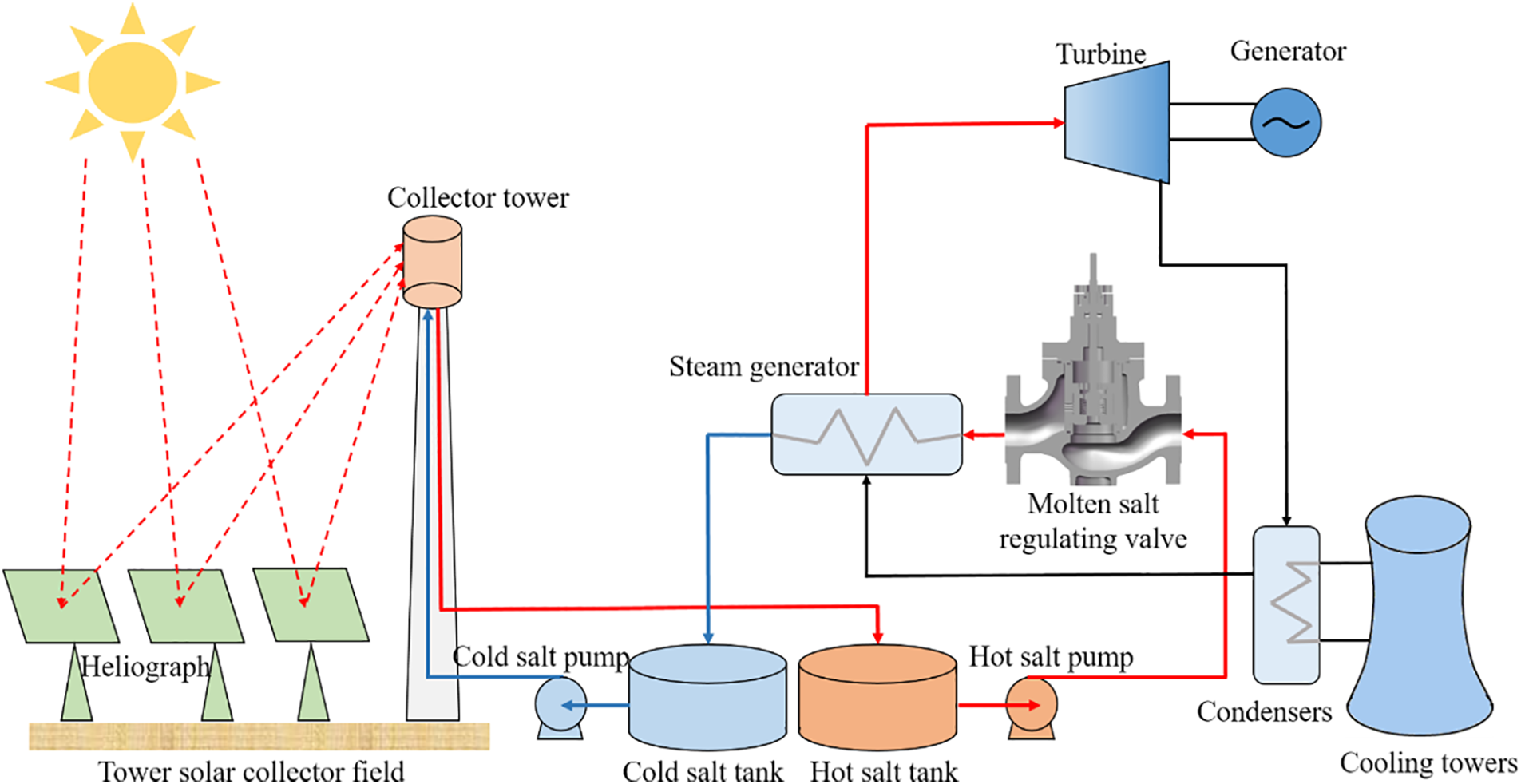
Figure 1: Tower solar thermal power generation system

To mitigate valve damage due to molten salt crystallization, it is generally advised against employing valve body structures that are prone to liquid accumulation within the valve cavity, such as gate valves and globe valves. Common regulating valve body forms can be divided into three types: the straight-through type, the angular type, and the direct-current type. The straight-through fluid has greater resistance because the shape of the valve body is similar to that of a sphere, it is also called a Globe-type valve body. Direct-current type valve bodies are mostly used for fluids containing solid particles or high viscosity, and right-angle valve bodies are used for right-angle pipelines. Globe valves are generally selected for small and medium-diameter valves in molten salt pipelines, while butterfly valves are also selected for large-diameter molten salt valves.

In the simulation study of purge gas-liquid two-phase flow to prevent molten salt crystallization, the conventional molten salt regulating valve body with the problem of aggregated liquid crystallization is taken as the research object. As shown in Fig. 2, the DN50 PN50 conventional molten salt regulating valve belongs to a Globe valve body structure.

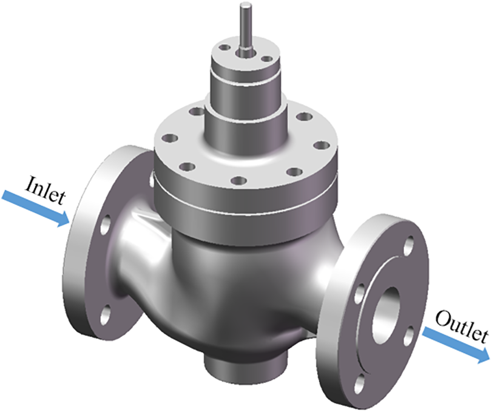
Figure 2: DN50 PN50 conventional molten salt pipeline regulating valve model

At present, the most commonly used heat transfer and heat storage molten salt in photothermal power plants is mainly composed of binary salts. Its maximum operating temperature and solidification temperature are relatively high. It is solid at standard temperature and atmospheric pressure, and the temperature rises to above the freezing point and converts into liquid [17]. In general, the conveying medium of the molten salt system is completely molten salt, and crystalline particles are precipitated when the temperature decreases. The formula of its physical parameters changing with temperature is shown in Eqs. (1) and (2) [18–20]:

ρsalt=2090−0.636tsalt (1)

μsalt=(22.714−0.120tsalt+2.281×10−4×tsalt2−1.474×10−7×tsalt3)×10−3 (2)

where ρsalt is molten salt density and its unit is kg/m3, tsalt is the temperature of molten salt and its unit is °C, μsalt is the dynamic viscosity of molten salt, and its unit is Pa·s.

The use temperature of binary salt is usually about 565°C, the corresponding molten salt density is 1730 kg/m3, the dynamic viscosity is 0.001144 Pa·s, and the surface tension coefficient of molten salt is 135 mN/m [21,22]. Upon system shutdown, compressed air is utilized to purge the pipeline and the molten salt valve, thereby expelling any accumulated molten salt. The recommended pressure for pipeline purging is 0.6~0.8 MPa. In this study, the simulated compressed air pressure is 0.7 MPa, the density is 8.6367 kg/m3, and the dynamic viscosity is 1.7853 × 10−5 Pa·s.

3  CFD Gas-Liquid Two-Phase Flow Numerical Simulation Theory and Method

3.1 Multiphase Flow Model

Presently, two numerical methodologies are employed to address multiphase flow: the Euler-Lagrange method and the Euler-Euler method. In the Euler-Euler method, different fluid phases are mathematically treated as interpenetrated continuous media. Given that one phase’s volume cannot be occupied by another, the notion of phase volume fraction is introduced. It is posited that these volume fractions are continuous functions of space and time, summing to unity. The conservation equations of each phase are derived, and a set of equations with similar structures for all phases is obtained. These equations are closed by providing a constitutive relationship based on empirical information. Fluent provides three different Euler-Euler multiphase models: the VOF model, the hybrid model, and the Euler model.

The first step to solve the multiphase flow problem is to correspond to the most realistic flow mode, and then select the appropriate model according to the degree of coupling between phases according to different flow modes. The VOF model is adept at handling flows characterized by distinct phase interfaces, whereas the Mixture and Eulerian models are more suitable for scenarios featuring phase mixing or separation, or when the volume fraction of the dispersed phase surpasses 10%.

The VOF model can model two or more immiscible fluids by solving a single set of momentum equations and tracking the volume fraction of each of the fluids throughout the domain. In this research, the fluid physical quantities can be obtained by solving the mass and momentum con-servation equations [23].

The mass conservation equation (namely, conti-nuity equation) reads:

∂∂t∫CVρdV+∫CSρ(u⋅n)dS=0 (3)

where ρ stands for the density, CS for the surface of control body CV, u for velocity vector and n for the normal vector of CS and points outward.

When the control body tends to be infinitesimal, Eq. (3) can be transformed into a coordinate-free form using Gauss’ divergence theorem:

∂ρ∂t+∇⋅(ρu)=0 (4)

Eq. (4) means that the divergence of u is zero for incompressible fluid. Thus, the fluid density is constant.

The momentum conservation equation can be described as follows:

∂(ρu)∂t+∇⋅(ρuu)=−∇p+∇⋅μ[(∇u+∇uT)−23∇⋅{u}I]+ρg+f + ∇⋅τRe (5)

where p denotes the pressure, μ is the viscosity, g is the gravitational acceleration vector, superscript T is the transposition notation, I is the unit tensor, f is the surface tension vector, and τRe is the Reynolds stress evaluated separately by means of a turbulence model. The continuum surface force (CSF) model was proposed by Brackbill et al. [24]. f denotes the surface tension source term added to the momentum equation.

f = σκ∇α (6)

κ=∇(∇α|∇α|) (7)

where σ and κ denote the interfacial tension and curvature, respectively.

The VOF model assumes that the pressure and velocity of each phase of fluid in a control volume are equal. The mixed fluid within the control volume is treated as a homogeneous flow, and the governing equation is solved for this mixture. The multiphase fluid calculation is accomplished by analyzing variations in the volume fraction of each phase within the mixed fluid. The volume equation for the qth phase in a mixed fluid is as follows [25]:

∂(ρqαq)∂t+∇⋅(ρqαqu)=0 (8)

In Eq. (8): ρq, αq represent the density and volume fraction of the qth phase fluid. u is the velocity of the mixed fluid. In the present case no mass transfer occurs between the two considered phases which explains why the right-hand side of Eq. (8) is set to zero.

Since the control body CV contains both gas-liquid phase components, the fluid density and viscosity can be expressed as simple linear combinations:

ρ=αgρg+αlρl (9)

μ=αgρg+αlρl (10)

αg+αl=1 (11)

where α denotes the volume fraction of phase component, subscript g and l represent gas phase and liquid phase respectively in this paper. Clearly, the control volume is exclusively filled with either gas or liquid, Consequently, the sum of the volume fractions of the gaseous and liquid phases equals one, which underscores the fluid’s continuity.

In the molten salt system, the accumulation of molten salt within the pipeline and valves is purged using compressed air. The valve flow manifests as gas-liquid contact, which parallels the stratified and free surface flow patterns characteristic of gas-liquid two-phase flow. The numerical simulation of this free liquid surface flow is challenging, primarily due to the complexity involved in tracking the free liquid surface. Consequently, the VOF model is hereby chosen for the subsequent computational simulations.

3.2 Three-Dimensional Turbulent Flow Model

The direct numerical simulation (DNS) method requires huge computational resources and is difficult to be extensively used in actual applications. Therefore, the Reynolds-averaged Navier-Stokes (RANS) method is proposed to effect time-averaging on the turbulent pulsation term, thereby mitigating computational complexity. However, the concomitant introduction of nonlinear terms engenders the non-closure of the N-S equations. Therefore, a variety of turbulence models are born, and the N-S equation is closed by introducing new equations.

(1) Turbulence models

In the numerical simulation of internal flow and purge of the molten salt control valve, including the influence of gravity, centrifugal force, and buoyancy, the backflow and secondary flow of the complex flow structure can be generated. To address the turbulence induced by rising bubbles, the Realizable k-ε model of Shih et al. [26]. Realizable k-ε model is suitable for complex shear flow involving large strain rates, vortex, secondary flow, and local excessive flow. In related studies, the Realizable k-ε model has been proved to have good applicability and calculation accuracy compared to other RANS models in the numerical simulation of gas-liquid two-phase flow [27,28].

Considering the complexity of the flow in the valve, the Realizable k-ε model is selected as the turbulence model in the numerical simulation of the internal flow and purge two-phase flow of the molten salt regulating valve.

(2) Turbulence model equations

The Reynolds time-averaged equation introduces the Reynolds stress term for the time-averaged treatment of the instantaneous N-S equation. The turbulence model is a specific relationship between the Reynolds stress and the time-averaged value. The two-equation model is the most extensively used turbulence model. The most basic two-equation model is the standard k-ε model, which adopts the following basic treatments: ① Using turbulent kinetic energy to reflect the characteristic velocity, ② Employing the turbulent kinetic energy dissipation rate to reflect the characteristic length scale, ③ Introducing the relation of turbulent viscosity μt=ρCμk2/ε , and ④ Being simplified by Boussinesq assumption.

The turbulent kinetic energy k equation can be expressed as:

ρ∂k∂t+ρui∂k∂xi=∂∂xi[(μ+μtσk)∂k∂xi]+Gk−ρε (12)

The turbulent kinetic energy dissipation rate ε equation can be expressed as:

ρ∂ε∂t+ρui∂ε∂xi=∂∂xi[(μ+μtσε)∂ε∂xi]+εk(c1Gk−c2ρε) (13)

where Gk is the production term of turbulent kinetic energy k due to the average velocity gradient, c1=1.44 and c2=1.44 refer to empirical constants, and σk=1.0 and σε=1.3 are the Prandtl numbers corresponding to turbulent kinetic energy k and dissipation rate ε, respectively.

Gk=μ{2[(∂ux∂x)2+(∂uy∂y)2+(∂uz∂z)2]+(∂ux∂y+∂ux∂x)2+(∂ux∂z+∂uy∂x)2+(∂uy∂z+∂uz∂y)2 (14)

In order to ensure positive normal force of the Reynolds stress, the Realizable k-ε model modifies the k-ε model and satisfies the Schwarz inequality:

ui2¯≥0 (15)

The Realizable k-ε model has two main improvements: ① As shown in Eq. (16), the coefficient Cμ in the turbulent viscosity calculation formula is related to the strain rate; ② The coefficient of the production term of the turbulent dissipation ε equation is changed from a constant to a function.

Cμ=1A0+ASU∗k/ε (16)

where A0, AS and U* are functions of the velocity gradient.

(3) Processing near the wall area

The turbulence model is efficacious primarily for fully developed turbulent flows. In the vicinity of walls, the presence of a boundary layer inhibits the full development of turbulence, necessitating specialized treatment methods to address the flow dynamics near the wall. The boundary layer is divided into three layers according to the different flow states. The flow core areas from the are the viscous bottom layer, the transition layer, and the turbulent core layer. In the viscous sublayer and the transition layer, the viscous force plays a leading role, and the viscous force is linearly related to the velocity gradient. Therefore, in the case of high Reynolds number turbulent flow in the core layer, the velocity distribution in the transition layer and the viscous sublayer can be directly calculated by the empirical formula. The characteristic parameters of the internal region of the turbulent boundary layer, dimensionless number y+ and dimensionless velocity u+, are introduced as shown in Eqs. (17) and (18):

y+=u∗yv (17)

u+=uu∗ (18)

u∗=τw/ρ (19)

τw=μ(∂u∂y)y=0 (20)

where u* is near-wall friction velocity and its unit is m/s, y is the distance between the first layer grid node and the wall surface and its unit is m, v is the kinematic viscosity of fluid and its unit is m2/s, u is fluid velocity and its unit is m/s, and μ is dynamic viscosity and its unit is kg/(m·s).

For the purpose of addressing the near-wall region, two principal methodologies are employed. Initially, the semi-empirical Wall Function approach is deployed to estimate the viscous influence region at the interface between the wall and the fully turbulent region, circumventing the requirement to explicitly solve the internal viscous influence region. Subsequently, the grid is refined, and the wall model method is implemented, which entails modifying the turbulence model to enable the resolution of the viscous sublayer and the transition layer.

In the wall treatment method, the standard wall function, the scalable wall function, and the non-equilibrium wall function are the wall function methods, which are suitable for high Reynolds number turbulence models (such as k-ε model, Reynolds stress model, etc.). The first layer of grid nodes is required to be in the turbulent core area, satisfying 30 ≤ y+ ≤ 300, and it is generally preferable for them to be near the lower bound of 30. The enhanced wall treatment is not a wall function method, which is suitable for low Reynolds number turbulence models (such as k-ω model, SA model, LES, etc.). It is necessary to divide a sufficiently fine grid in the near wall region, which requires the first layer of grid nodes to be located in the viscous sublayer, that is, y+ < 5, and the number of boundary grid layers is required to be at least 10 layers. For simple shear flow problems, the standard wall function method is adept at providing solutions, while the non-equilibrium wall function method enhances the calculation of flows with strong pressure gradients and separation. Furthermore, the scalable wall function approach ameliorates computational instability issues that arise from oscillations between the viscous sublayer and the core layer during the iterative calculation process of the initial grid node layer. The enhanced wall treatment is usually used for complex flow problems where the logarithmic law cannot be applied. Therefore, the non-equilibrium wall function method is selected in the numerical simulation of gas-liquid two-phase flow in anti-crystallization purging of molten salt regulating valve.

3.3 Dynamic Grid Adaptive Method

When employing dynamic grid adaptation for transient solution calculation, a certain area is dynamically encrypted according to a certain method to achieve high-precision capture of physical variables in the area. During the purging process of the molten salt regulating valve, the continuous fluid will be purged into small liquid clusters or even droplets, with their size and position changing constantly. At this time, the dynamic grid adaptive method is to track liquid accumulation sites, with grid refinement focused on accurately depicting the accumulation’s morphology and local physical variables. Through the dynamic grid adaptive method, the number of grids in the whole model can be considerably reduced, and the calculation convergence time can be shortened under the premise of capturing the liquid droplets sufficiently.

(1) Adaptive grid refinement

There are two types of adaptive methods in Fluent: Hanging node Adaption and Polyhedral Unstructured Mesh Adaption (PUMA).

(2) Application of grid adaptive method

The grid adaptation process can be divided into two important parts: Firstly, the advantages and disadvantages of the grid are determined according to the adaptive function established based on geometric and computational data. Then, the grid is modified to optimize the grid.

4  CFD Numerical Simulation of Gas-Liquid Two-Phase Flow in Molten Salt Regulating Valve

The purging of liquid accumulation in molten salt regulating valves presents a complex gas-liquid two-phase flow, which is inherently challenging to resolve and often leads to issues of stability and convergence. In order to accurately simulate multi-phase flow, the convergence of two-phase flow simulation can be improved from model processing, grid partition, boundary condition setting, calculation control condition setting, and other aspects. The flow chart of the gas-liquid two-phase flow calculation is shown in Fig. 3.

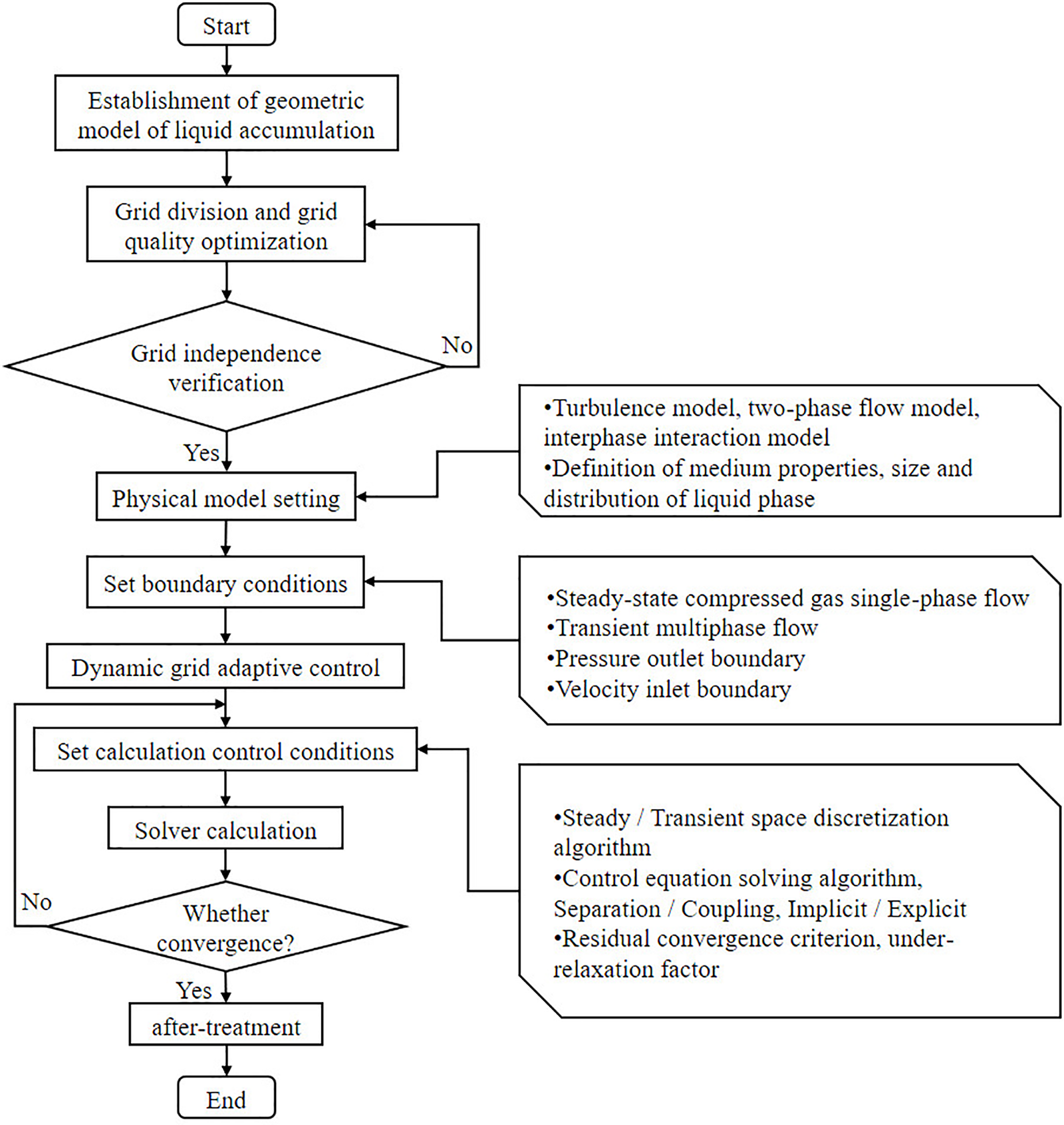
Figure 3: CFD simulation calculation process of gas-liquid two-phase flow

4.1 Grid Partition and Grid Independence Verification

The geometric model of the fluid accumulation in the flow channel can be assigned to the fluid domain in two distinct approaches. The first method involves the meshing and marking of the liquid accumulation zone during the Fluent setup resolution. The subsequent method encompasses the segmentation of the flow channel model during the pre-processing phase to delineate the fluid accumulation region, which is subsequently initialized as a liquid molten salt medium within the Fluent solution environment.

In order to ensure the accuracy of the calculation, it is imperative that the fluid flow within the channel is fully developed. Therefore, the pipe with 5 times the nominal diameter length is added before and after the valve, and the flow channel model is generated by reverse modeling according to the three-dimensional solid model. As shown in Fig. 4, the bottom of the flow channel groove is segmented to establish the liquid accumulation area in SCDM, and the regions of the model are topologically shared. When the flow channel depth H is 62 mm, and the determining parameter H0 of the liquid accumulation height is 45 mm, the liquid accumulation height is 17 mm.

Figure 4: Liquid accumulation model of conventional molten salt regulating valve flow channel

As shown in Fig. 5, the fluid domain grid of the molten salt regulating valve is generated using Fluent Meshing software. The polyhedral grid boasts superior generation efficiency and adaptability, rendering it apt for meshing complex geometries. Size functions such as Curvature and Proximity are suitable for capturing small curved surfaces and large span grid generation of gap geometric features. At the same grid resolution, the polyhedral grid entails a reduced number of elements.

Figure 5: Grid partition of fluid domain of conventional molten salt regulating valve

The pipeline fluid area at the front and rear of the valve, the liquid gathering area at the bottom of the valve, and the upper fluid area of the valve are connected in the form of separate interfaces. The splicing between the polyhedron grids is conformally mapped, and the nodes are in one-to-one correspondence. The internal surface is designated as a flow-flow boundary to facilitate fluid traversal across the shared interface. Considering the influence of the boundary layer, the wall function approach is employed for the near-wall treatment, with a y+ value of 30. Therefore, the grid height of the first layer is set to be 0.13 mm on the surface of the valve body and the pipe, with a total of 5 layers, and the grid growth factor is 1.2.

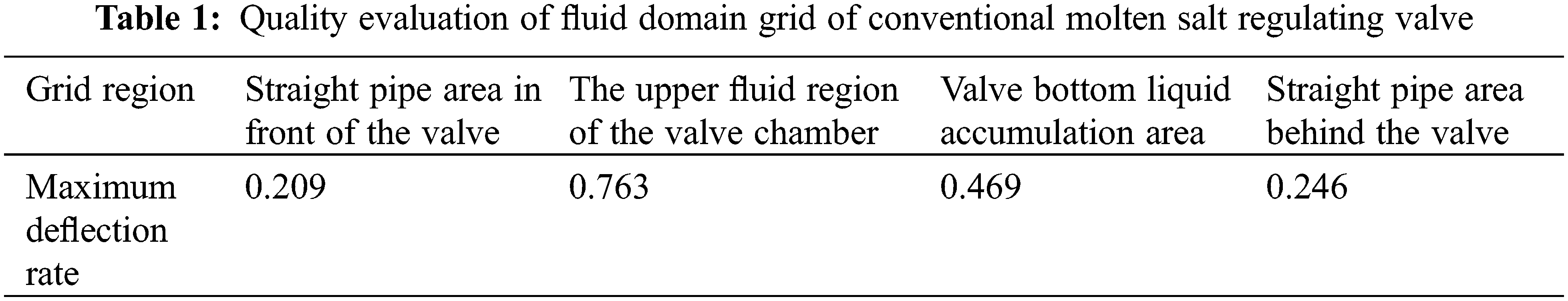
The maximum deviation rate evaluates the grid quality of each area, and the evaluation results are shown in Table 1. The results satisfy the criterion that the maximum deflection rate for CFD simulations should not exceed 0.90.

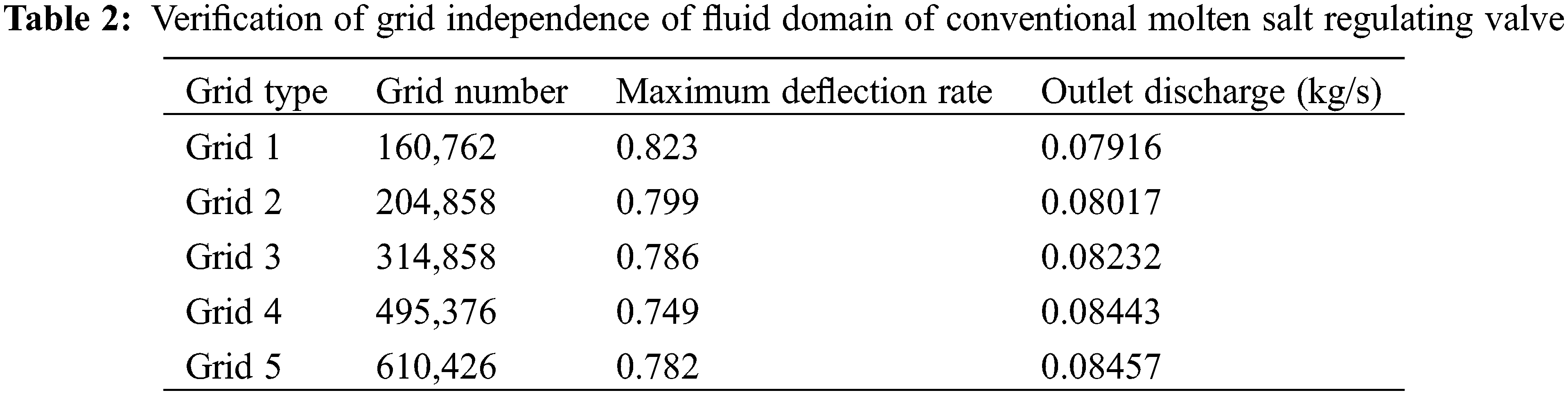
The Reynolds number inside the valve far exceeds the critical Reynolds number. The turbulence model is used to study the flow in the valve. The steady-state calculation of the single-phase flow of compressed air is carried out at the inlet velocity of 5 m/s. The grid independence verification is performed with the outlet flow value as the target, as shown in Table 2. The number of grids from grid type 3 to grid type 4 increases by 57%, the flow increases by 2.6%, the number of grids from grid type 4 to grid type 5 increases by 23.2%, and the outlet flow value increases by 0.17%. Once the grid count surpasses 495,000, the flow value exhibits stability with further increments in grid quantity. Therefore, a grid count of approximately 495,000 is chosen for the CFD simulation.

4.2 Solution Calculation and Convergence Control of Purge Gas-Liquid Two-Phase Flow

Fluent double-precision calculation is used for the transient calculation of two-phase flow. The turbulence model is Realizable k-ε. The inlet adopts the velocity inlet boundary condition and sets the initial gauge pressure. The outlet adopts the pressure outlet boundary condition, and the outlet gauge pressure is set to 0. In order to improve the convergence of calculation, the steady-state calculation of single-phase flow of compressed air is carried out for a stable initial flow field. Subsequently, the liquid accumulation is designated as the secondary phase, while compressed air is considered the primary phase. The transient simulation proceeds with a time step of 0.00001 s and automatically archives data every 0.0005 s.

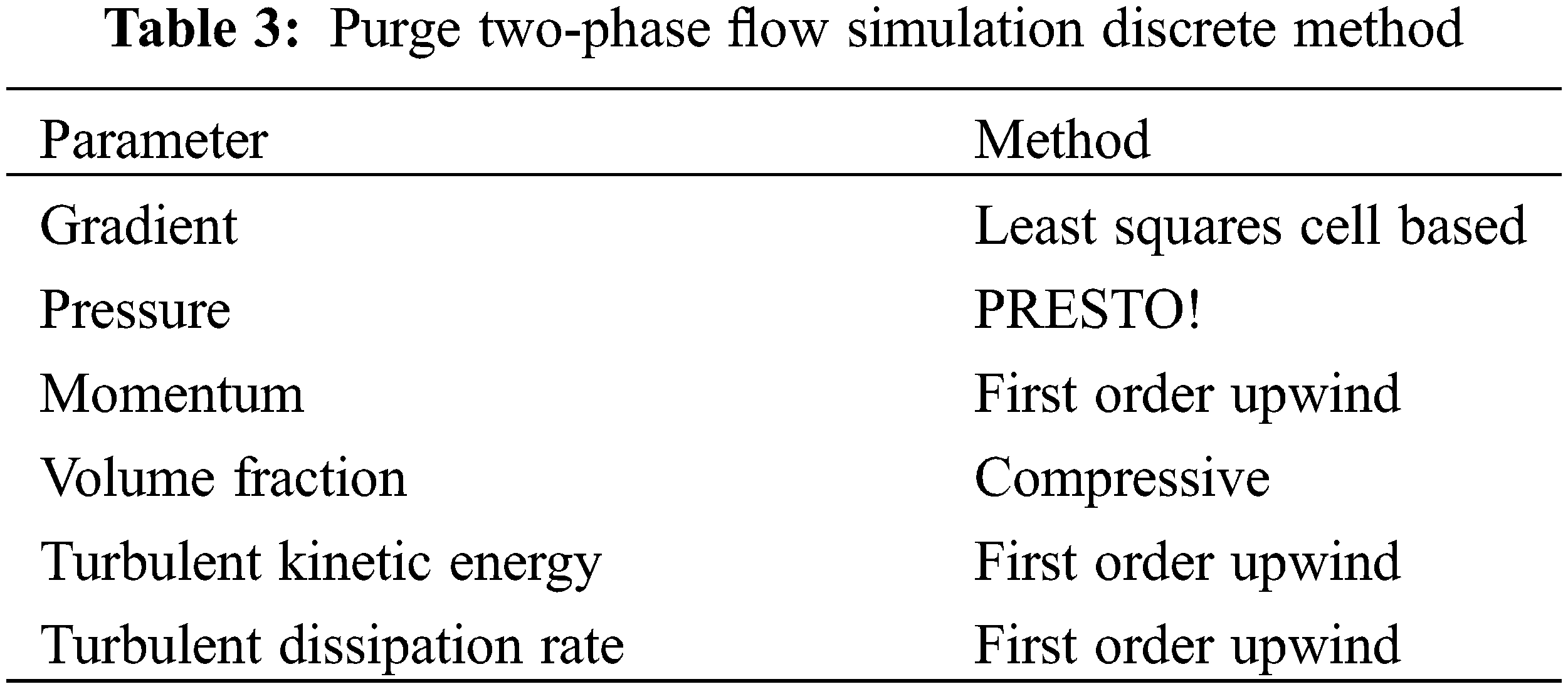
The VOF model is deployed to analyze the purge two-phase flow, favoring a type conducive to convergence and accounting for surface tension in inviscid analysis. Balancing computational accuracy with efficiency, the spatial and temporal discretization follows the scheme outlined in Table 3, with the PISO algorithm selected for resolving pressure-velocity coupling.

The steady-state VOF two-phase flow calculation can be used when only focusing on the final state of the liquid accumulation purge, such as comparing the final effect of purge under different gas flow rates or different initial liquid accumulation mass. The Coupled pressure-velocity coupling algorithm and the pseudo-transient method are selected. The iteration step is 1500 steps. In the steady-state solution process, the convergence cannot be solely judged based on the residual error. Concurrently, the mass of liquid accumulation within the designated region must be vigilantly monitored until the value remains essentially constant.

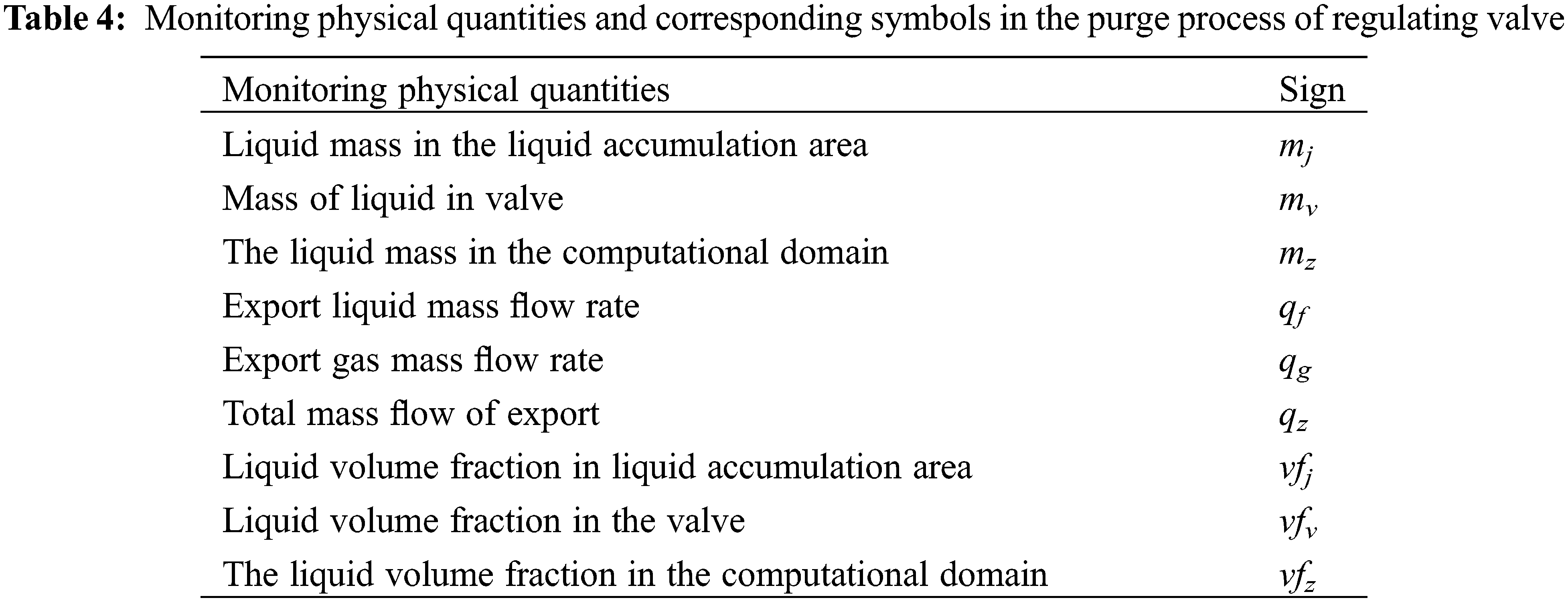
The transient solution process involves monitoring the liquid mass across the calculation domain, within the valve, and in the liquid accumulation area, as well as the outlet liquid flow and the liquid volume fraction in these regions, to analyze the liquid’s dynamic changes during the purge process. The specific parameters and codes are shown in Table 4. In the subsequent molten salt liquid purge study, the remaining molten salt liquid mass in the valve is expressed as mvr, and the outlet molten salt mass flow rate is expressed as qr.

In order to accurately simulate multiphase flow, the convergence improvement methods of two-phase flow simulation are summarized from four aspects: model processing and grid quality control, general solution control, two-phase flow solution control, and solution format control.

(1) Model processing and grid quality control

The premise of high-precision simulation of two-phase flow is model processing and grid quality control. Reasonable simplification of the model can improve the efficiency of grid partition and grid quality, and avoid the influence of grid number on the calculation results through grid independence verification. Grid problems mainly include topological connection problems and grid quality problems. The grid processing flow involves geometric model repair, surface grid quality diagnosis optimization, and volume grid quality optimization. Fluent meshing provides a grid inspection and optimization tool. During grid partitioning, a hybrid approach is employed that integrates traditional grid inspection with process-based partitioning methods. This synergy leverages the flexibility of the traditional mode and the convenience of the process-oriented approach, thereby enhancing the efficiency of grid partitioning.

In order to ensure the quality of the grid, the distortion degree should be controlled with 0.9, with an optimal target of 0.85 or less. At the same time, the grid should be reasonably refined to ensure the reasonable distribution of grid density, and there are dense grid elements in the complex flow area. The boundary layer region should meet the y+ numerical requirements corresponding to the turbulence model.

(2) General solution control

① To ensure the reliability of the transient two-phase flow simulation, a convergent steady-state initial flow field is first computed, excluding the volume fraction equation. Subsequently, the liquid accumulation area is defined to initiate the two-phase flow calculation. This procedure circumvents convergence issues stemming from backflow at the outlet, which could otherwise yield unreliable solutions. ② In instances of unstable and divergent solutions, the relaxation factor can be reduced. ③ The time step can be initially set to a smaller value, with subsequent increments applied after several iterations to more effectively approximate the pressure field.

(3) Two-phase flow solution control

① Considering the volume force, in the case of a large volume force, the Implicit Body Force is selected to improve the convergence of the solution by solving the partial balance of the volume force in the pressure gradient and momentum equation, so that the flow can quickly establish a realistic pressure field. ② The reference pressure position is located in the region with the smallest fluid density, and the operating density takes the density value of the light phase, which can reduce the rounding error and improve the convergence stability.

(4) Solving format control

① The PISO velocity-pressure coupling scheme considerably reduces the number of iterations required to achieve convergence. ② The choice of discrete format, such as volume fraction discrete format, chooses Compressive for high precision and medium speed.

4.3 Accuracy Verification of CFD Purge Gas-Liquid Two-Phase Flow Numerical Simulation Method

Akhlaghi et al. [29] used the multi-fluid VOF model to simulate the intermittent flow of air-water in horizontal pipes, and carried out visualization experiments under the same flow conditions. The gas-water interface structure was qualitatively evaluated, and the fluid velocity and pressure drop were quantitatively evaluated. The results show that the multi-fluid VOF model is consistent with the visualization experiment results.

The gas-liquid two-phase flow process in the horizontal pipeline in reference [29] is numerically simulated using the CFD gas-liquid two-phase flow numerical simulation method of purging the molten salt regulating valve used in this paper. The verification simulation is carried out in a pipeline with an inner diameter D of 44 mm and a length of 137D. The liquid phase was injected from the peripheral pipe, and the gas phase was injected from the middle area pipe. The velocity of the peripheral liquid phase follows the power law curve, and the gas phase flows at a uniform velocity in the core area of the inlet of the pipeline. The velocity distribution at the inlet boundary is shown in Eqs. (21) and (22):

ug=Ajgπrg2;φg=1,φl=0;0≤r≤rg (21)

ul=ucl(1−rR)17;φg=0,φl=1;rg<r≤D2 (22)

where A is pipeline cross-sectional area and its unit is m2, jg is gas phase apparent velocity, and its unit is m/s.

rg and ucl are calculated as shown in Eqs. (23) and (24):

rg=7R(jg+225jg2+240jgjl)8(14jg+15jl) (23)

ucl=60Ajl7π(1−rgR)1/7(7R2+Rrg−8rg2) (24)

where jl is the liquid phase apparent velocity, and its unit is m/s. In the verification simulation, jl is 1 m/s, and jg includes 1.64 and 0.16 m/s, respectively.

As shown in Fig. 6, the fluid domain model consistent with the literature is constructed, followed by grid partitioning and grid independence verification.

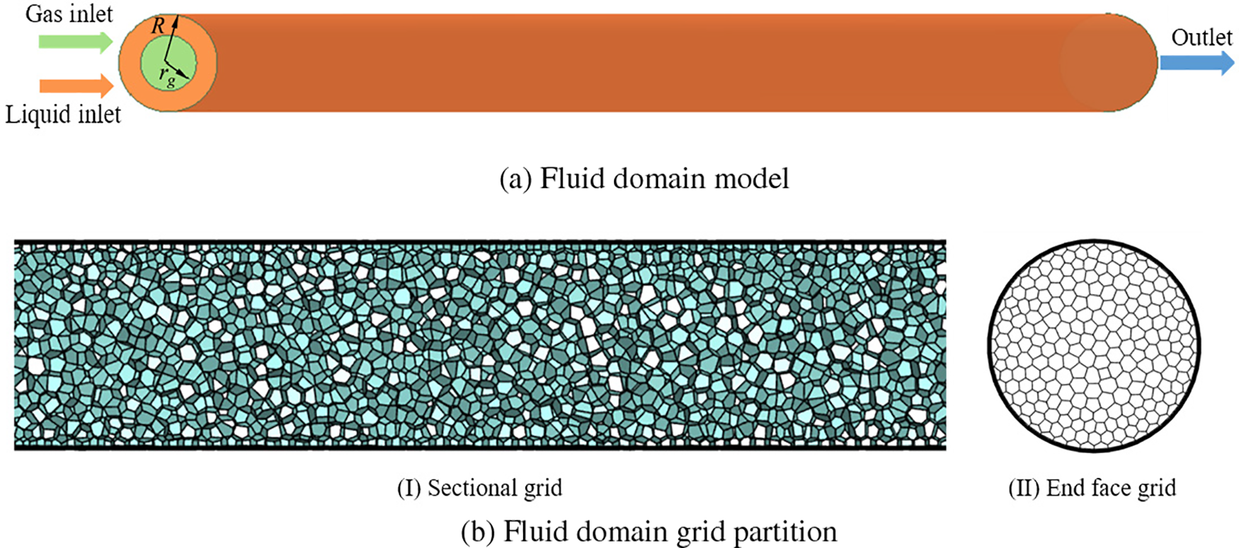
Figure 6: Corresponding to the fluid domain model establishment and grid partition in the literature

The experimental and simulation parameters indicate air density and dynamic viscosity of 1.184 kg/m3 and 1.844 × 10−5 kg/(m·s), respectively, while water density and dynamic viscosity are 996.5 kg/m3 and 8.684 × 10−4 kg/(m·s), respectively. The air-water surface tension coefficient is 0.072 N/m. The flow field is initialized with liquid.

According to the transient CFD gas-liquid two-phase flow simulation method, the solved working condition jg is 1.64 m/s, and jl is 1 m/s. The numerical simulation of the gas-liquid interface is compared with the results in the literature, as shown in Fig. 7. Fig. 7a presents the comparison between the visual experimental gas-liquid interface taken by the high-speed camera in the literature and the numerical simulation of the gas-liquid interface in the literature. Fig. 7b depicts the verification simulation result using the research method in this paper. The proximity of the three values indicates the reliability of the CFD gas-liquid two-phase flow simulation method in simulating the anti-crystallization purge of molten salt control valves for flow state representation.

Figure 7: Comparative verification of gas-liquid interface literature

Fig. 8 presents a comparison of the velocity results when jg and jl are 0.16 and 1 m/s, respectively, 50D section from the inlet of the pipeline and t = 1.6 s. Fig. 8a shows the velocity curves of the 50D profile under different grids in the literature, with the Mesh (c) independence test confirming grid acceptability. Fig. 8b illustrates the velocity of the 50D profile obtained after verifying the grid independence test in the simulation.

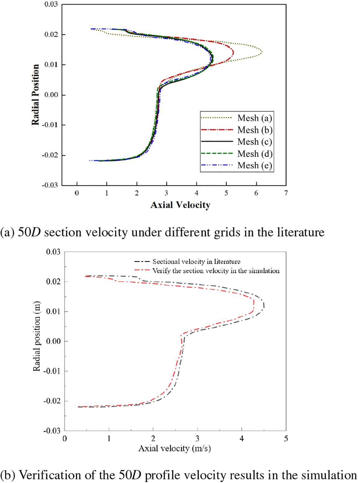
Figure 8: Comparison and verification of speed results

The simulation’s profile velocity results deviate by a maximum of 5% from those in the literature, indicating high accuracy. This confirms that the CFD gas-liquid two-phase flow simulation method used in this study is precise and reliable for modeling flow regimes and parameters, and is thus suitable for analyzing gas-liquid two-phase flow in the anti-crystallization purging of molten salt regulating valves.

5  Study on Numerical Simulation and Purge Characteristics of Molten Salt Regulating Valve Liquid Purge

5.1 Purge Numerical Simulation Control Experiment Design

In order to delve into the effects of purge gas flow rate, initial liquid mass, purge time, and flow channel profile curve at the bottom of the valve body on purge efficiency, the following four groups of control experiments are designed through trial calculations:

(1) Simulation experiment group 1: In order to compare and analyze the influence of purge gas flow rate on purge efficiency, four groups of the initial liquid height of 17 mm and purge gas flow rate Ug of 1, 3, 5, and 10 m/s are designed to simulate the steady-state liquid accumulation purge two-phase flow process and monitor the mass convergence process of residual liquid accumulation.

(2) Simulation experiment group 2: In order to compare and analyze the influence of initial liquid mass on purge efficiency, the initial liquid height is set at 10, 17, 22, and 27 mm, respectively, and the purge gas flow rate Ug is 1, 3, and 5 m/s, respectively. A total of 12 groups are involved to simulate the two-phase flow process of steady-state liquid accumulation purge and monitor the convergence process of residual liquid mass.

(3) Simulation experiment group 3: In order to compare and analyze the influence of purge time on purge efficiency, the initial liquid height is designed to be 17 mm, and the purge gas flow rate Ug is 1, 3, 5, and 10 m/s, respectively. A total of 4 groups are included to simulate the transient liquid purge two-phase flow process, and all the physical quantities in Table 4 are monitored.

(4) Simulation experiment group 4: As shown in Fig. 9, the spline curve is used to improve the flow channel profile at the bottom curve of the valve body in Fig. 2, reduce the depth of the flow channel, move the horizontal distance of the lowest point of the flow channel to the left, and increase the arc curvature of the flow channel. In order to compare and analyze the influence of the flow channel profile at the bottom of the valve body on the purging efficiency, the initial liquid height is designed to be 17 mm, and the purge gas flow rate Ug is 1, 3, and 5 m/s, respectively. The simulation of the steady-state two-phase flow during liquid accumulation purge is conducted to track the convergence of residual liquid mass.

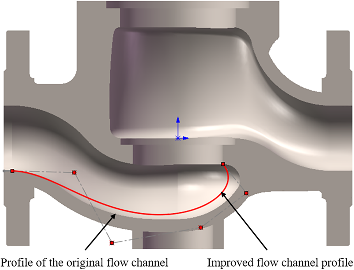
Figure 9: Improvement of flow channel profile of conventional molten salt regulating valve

Table 5 delineates the experimental items and corresponding boundary conditions of the control experiment design for the numerical simulation of the molten salt regulator valve purge.

The experimental definition takes the mass of liquid blown out after purging as a percentage of the initial mass of liquid in the valve as the purging efficiency, as shown in Eq. (25):

η=mbmi% (25)

mb=mi−mr (26)

where η is the purging efficiency, mb is the blown liquid mass, mi is the initial liquid mass, and mr is the remaining liquid mass in the valve after purging.

5.2 Analysis of Dynamic Flow Field Results in the Purge Process

Taking the transient calculation process of the initial liquid accumulation height of 17 mm and the purge gas flow rate of 3 m/s in the simulation experiment group 3 as an example, this analysis investigates the three-dimensional dynamic flow field visualization during the liquid loading purge process. It examines the dynamic grid adaptation, velocity streamlines, three-dimensional volume fraction, and the distribution and variation of vorticity throughout the purge process.

(1) Dynamic grid adaptive analysis

Fig. 10 presents the dynamic adaptive grid and volume fraction cloud map at 0.05 s of the liquid accumulation purge process.

Figure 10: Dynamic grid adaptation at 0.05 s

Grids are refined when they contain liquid, and coarsened when the gas-liquid interface crosses them, nearly devoid of liquid, to optimize computational resources and reduce computational load. The dynamic grid adaptation process, as illustrated in the figure, enables the capture of critical details with a reduced grid count, enhancing solution accuracy and accelerating computation.

(2) Analysis of liquid volume fraction in dynamic process valve

Visualization of volume fraction changes during the molten salt liquid purge process is achieved using the volume rendering method. As shown in Figs. 11 to 13, the entire process can be divided into the initial violent surge stage, the discharge stage, the partial fall stage, and the liquid dissipation stage.

Figure 11: Initial violent surge stage

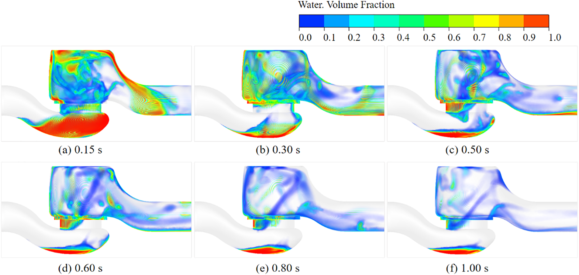
Figure 12: Discharge and partial fall stage

Figure 13: Liquid dissipation stage

As shown in Fig. 11, the initial violent surge stage ranges within 0~0.10 s, and the molten salt liquid is mainly in the valve body area. At 0 s, the compressed air does not enter the valve, and the liquid level of the liquid accumulation is stable. When the compressed air is introduced, the liquid surges to the upper part of the valve cavity and diffuses in the lower flow channel. At 0.1 s, most of the liquid enters the upper part of the valve cavity and surges to the outlet.

As shown in Fig. 12, during the period of 0.10~1.00 s, it is the discharge and partial fall stage. During this interval, a portion of the liquid is expelled through the valve outlet, resulting in a decrease in the liquid level in the upper part of the valve cavity, while another part of the liquid retreats back into the lower flow channel.

Fig. 13 depicts the liquid dissipation stage between 1.00 and 2.50 s, where the liquid in the upper valve chamber is entirely purged from the valve by compressed air, and the liquid accumulation in the lower flow channel exhibits minimal change. Steady-state calculations confirm that the liquid cannot be completely emptied under the condition of 3 m/s purge gas flow rate.

(3) Velocity streamline analysis

Fig. 14 depicts the velocity streamline diagram of the liquid loading purge process under the condition of 3 m/s purge gas flow rate. The velocity and streamline distribution also reflect the movement of the liquid during the purge process. For example, the velocity of the lower part of the valve chamber at 0.04 s is in the range of 2.0~3.5 m/s. In comparison, as shown in Fig. 11c, it can be found that the 0.04 s moment belongs to the initial violent surge stage, and the liquid moves rapidly to the upper part of the valve chamber along the flow channel under the action of compressed gas.

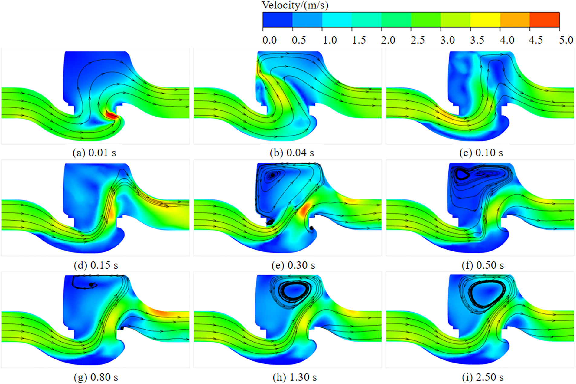
Figure 14: 3 m/s working condition streamline diagram

(4) Analysis of vortex evolution process

Accurate identification of vortex structures holds considerable significance for understanding flow mechanisms, solving turbulence problems, and conducting flow control. Intuitively, the vortex represents the rotational motion of the fluid [30]. In order to better explore the evolution mechanism of the liquid accumulation purge in the valve, the relationship between the liquid accumulation distribution and the vortex is discussed by referring to the Q criterion of the three-dimensional structure of the vortex.

The Q criterion is the most commonly used vortex identification method. The second Galilean invariant Q > 0 of the velocity gradient tensor ∇V is used to represent the vortex structure. The Q expression is [31]:

Q=12(||B||F2−||A||F2) (27)

where ||·||F is the Frobenius norm of matrix, and A and B are the symmetric part and the antisymmetric part of the velocity gradient tensor, respectively.

The anti-symmetric vortex tensor exceeds the symmetric strain rate tensor in the fluid region, denoted as Q > 0, signifying the presence of a vortex; the converse implies the absence of a vortex.

Fig. 15 compares the liquid volume fraction during the purge of liquid accumulation with the vortex core, with the vortex core visualized in terms of liquid volume fraction. At the onset of the simulation (0.02 s), high-pressure gas drives the accumulation of liquid to the bottom left dead zone of the valve body, where the liquid volume fraction reaches approximately 0.95, coinciding with the location of the vortex core, which also exhibits a volume fraction of about 0.95. By 0.04 s, the liquid ascends into the upper region of the valve body, impacting the upper right wall with a maximum volume fraction of approximately 0.9. The vortex core remains in the bottom right dead zone of the valve body, showing a diffusion phenomenon within its core region. At 0.10 s, the liquid is expelled from the valve body, and the vortex core diffuses across most of the valve body region, still centered in the bottom dead zone. The proliferation of the liquid vortex nucleus is accompanied by a diffusive distribution pattern. The analysis reveals a strong correlation between the vortex core structure and the volume fraction at different times.

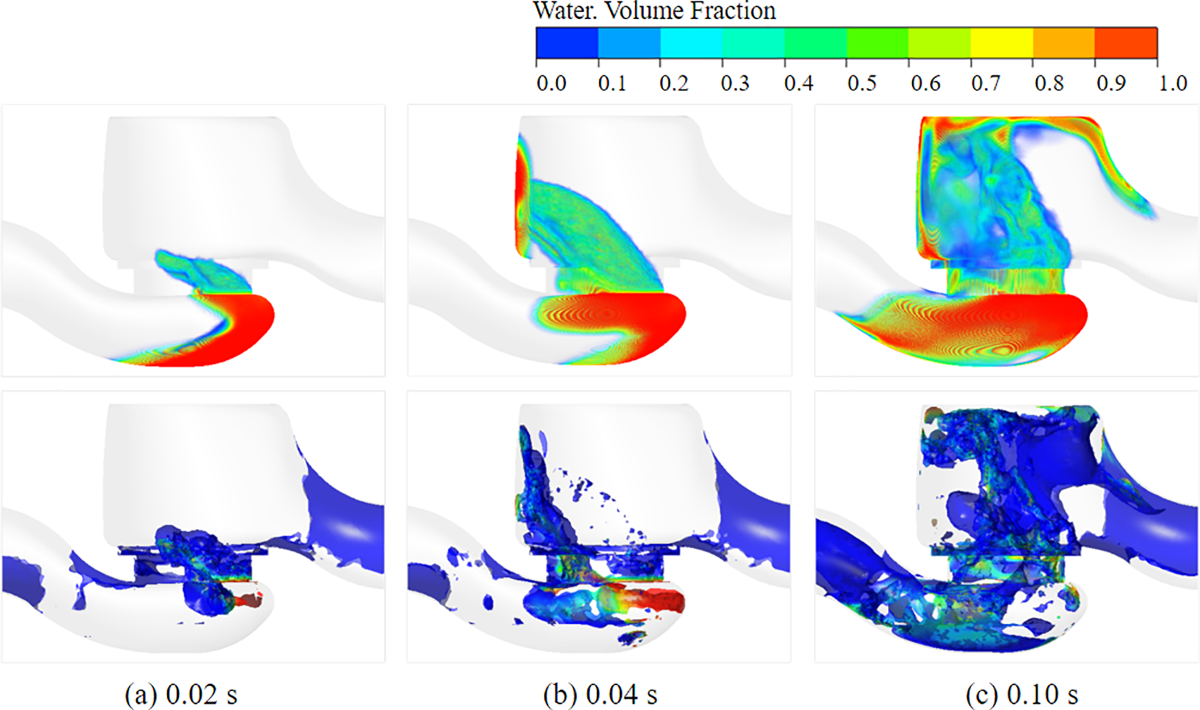
Figure 15: Comparison diagram of volume fraction and vortex core

5.3 Numerical Simulation Experimental Analysis of Purging of the Molten Salt Regulating Valve

(1) The influence of different flow velocitys on purge efficiency

The steady-state simulation method of liquid accumulation purge two-phase flow is employed to calculate various working conditions of simulation experiment group 1. The convergence curve of residual liquid mass is shown in Fig. 16, and the calculation reaches convergence at the iteration step of 1500 steps. The results of CFD calculations at different gas flow rates are summarized in Table 6.

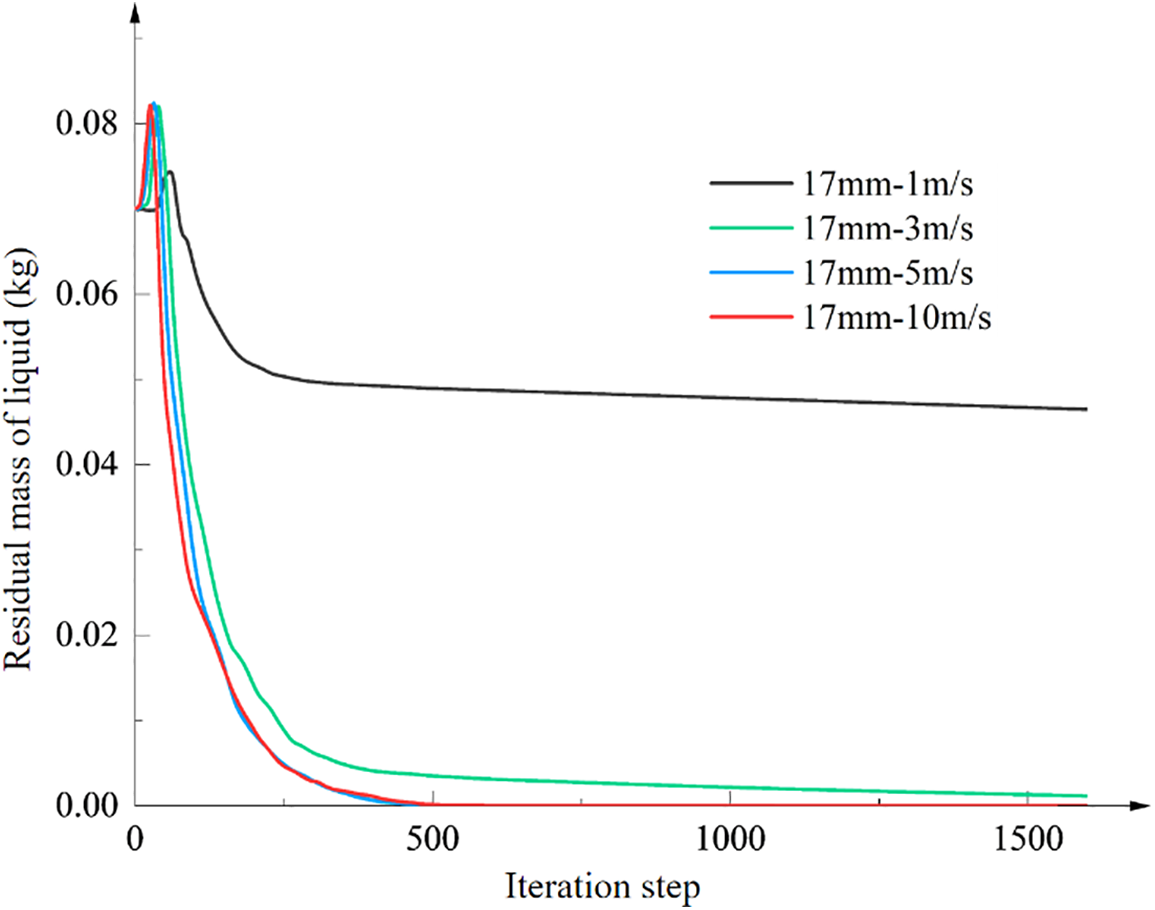
Figure 16: Convergence curve of residual liquid mass at different gas flow rates

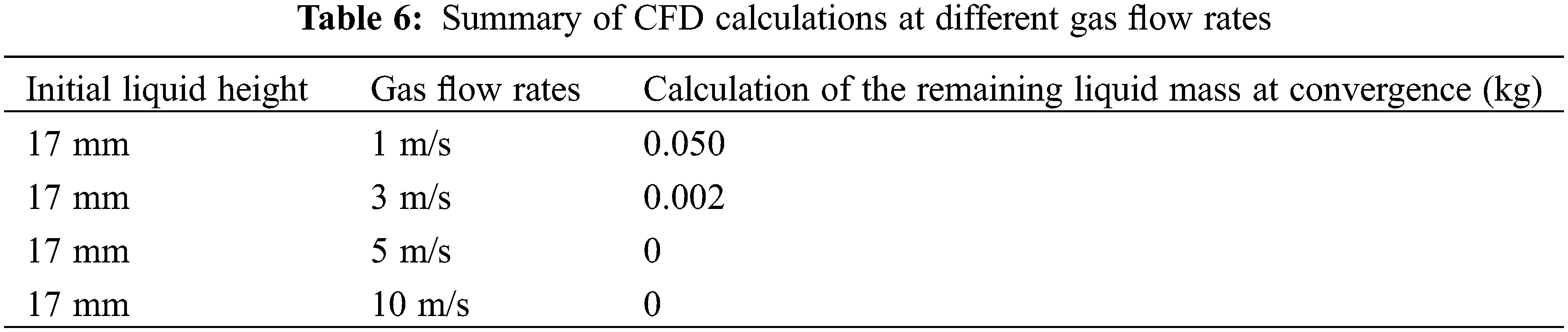
According to Fig. 16 and Table 6, for an initial liquid height of 17 mm, there exists a critical purge flow rate within the range of 3 to 5 m/s. An important conclusion is drawn from the analysis of different purge gas flow rates: There is a critical purge flow rate in the liquid accumulation purge process. Only when the purge gas flow rate exceeds the critical purge flow rate can the liquid accumulation be completely discharged.

(2) Influence of different initial liquid mass on the purge efficiency

The steady-state simulation method of liquid accumulation purge two-phase flow is employed to calculate various working conditions of simulation experiment group 2. The convergence curve of residual liquid mass is shown in Fig. 17, and the calculation reaches convergence at the iteration step of 1500 steps. The results of CFD calculations for different initial liquid accumulation mass are summarized as shown in Table 7.

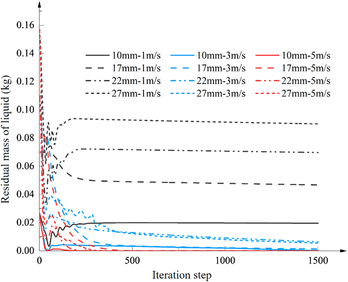
Figure 17: Residual liquid mass convergence curve after purge under different initial liquid accumulation mass

At a purge gas flow rate of 1 m/s, the four initial liquid accumulation mass conditions fail to completely evacuate the liquid, resulting in a substantial residual liquid mass. At initial liquid accumulation heights of 10, 17, 22, and 27 mm, the purging efficiencies are 26.0%, 33.4%, 36.5%, and 42.6%, respectively. However, at the gas purge flow rate of 3 m/s, while the four initial liquid conditions cannot completely empty the liquid, the residual liquid mass is rather small. At initial liquid accumulation heights of 10, 17, 22, and 27 mm, the purging efficiencies are 98.85%, 98.12%, 94.13%, and 96.48%, respectively, indicating that 3 m/s approximates the critical purge flow rate. At the purge gas flow rate of 5 m/s, complete liquid evacuation is achieved across all four initial liquid accumulation conditions, indicating that 5 m/s exceeds the critical purge flow rate.

From the analysis of different initial liquid accumulation masses, it is concluded that: ① When the purge gas flow rate Ug is less than the critical purge flow rate UC, the initial liquid accumulation mass is proportional to the residual liquid mass. ② When the purge gas velocity Ug approximates the critical purge flow rate UC, the initial liquid accumulation mass has little effect on the residual liquid mass. ③ When the purge gas flow rate Ug exceeds the critical purge flow rate UC, the initial liquid accumulation mass does not affect the residual liquid mass. ④ The critical purge flow rate UC has nothing to do with the initial liquid mass.

(3) Influence of purge time on purge efficiency

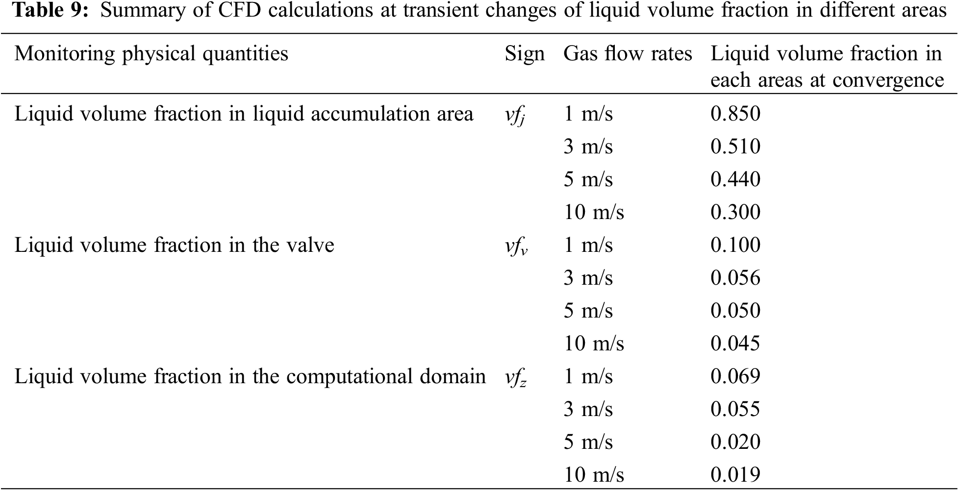
The transient-state simulation method of liquid accumulation purge two-phase flow is used to calculate various working conditions of simulation experiment group 3, and the variation of liquid mass, volume fraction, and outlet flow rate in each region during the transient process of liquid purge is analyzed, as shown in Figs. 18–20. A summary of the CFD calculation results is shown in Tables 8 and 9.

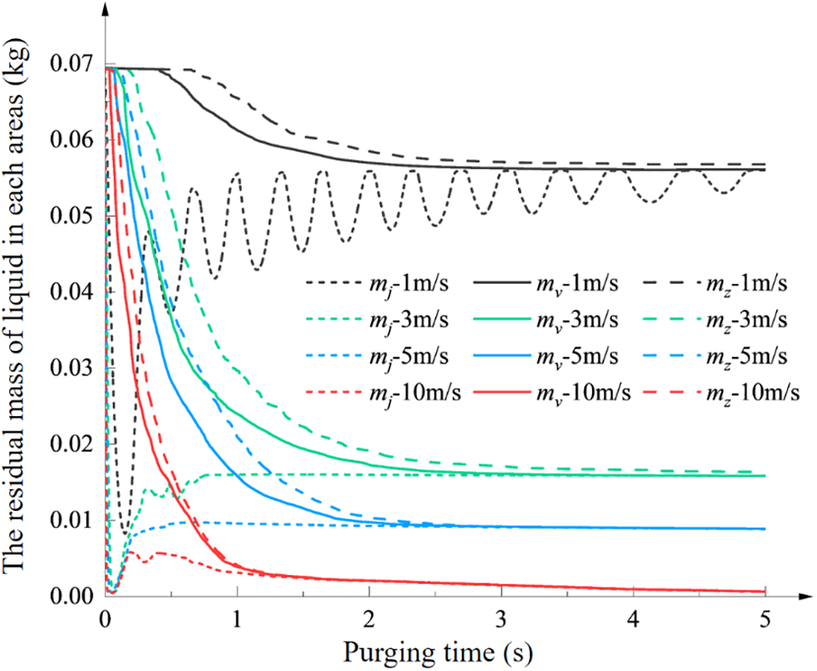
Figure 18: Transient changes of residual liquid mass in different areas

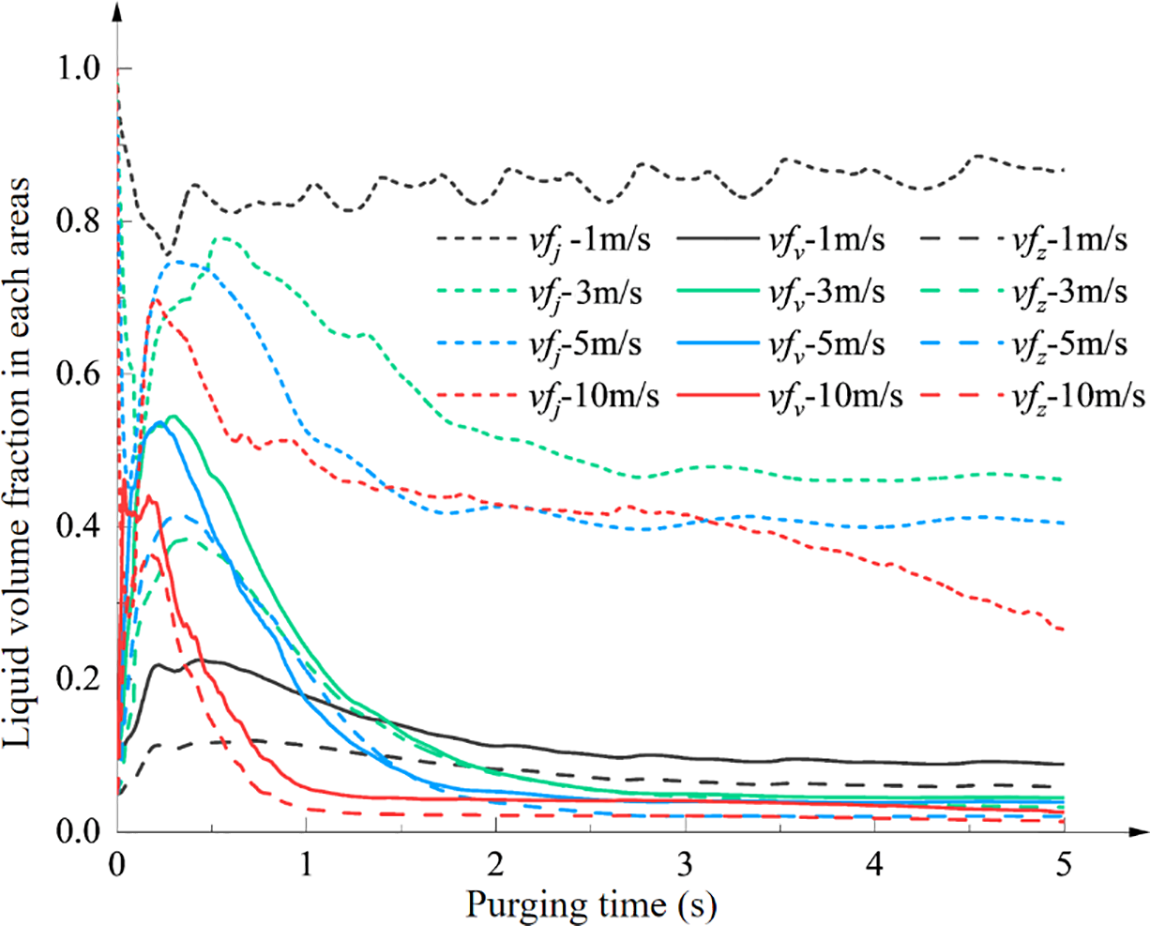
Figure 19: Transient changes of liquid volume fraction in different areas

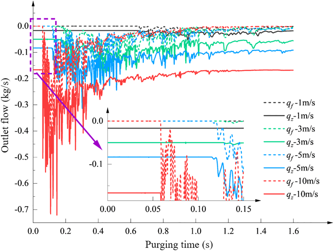
Figure 20: Transient variation of the outlet flow rate of different media

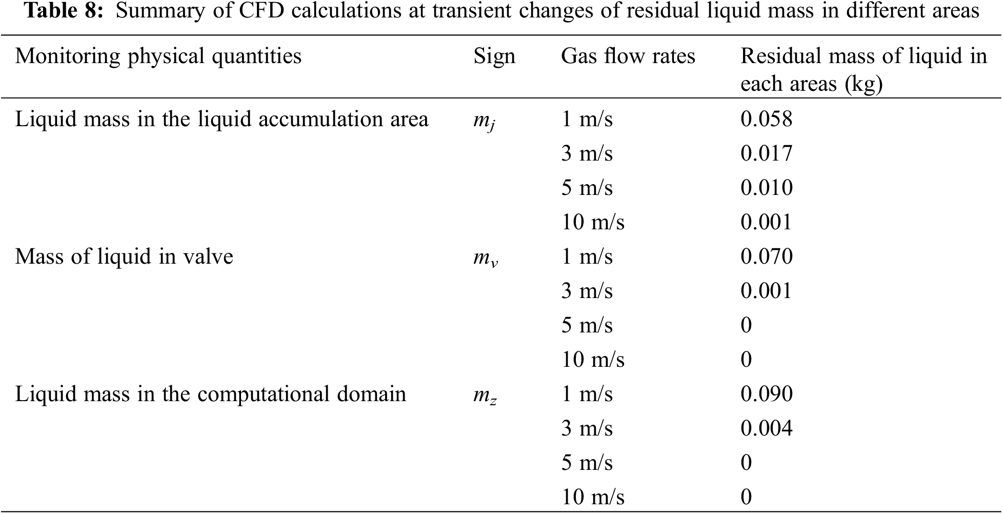
From the analysis of Fig. 18 and Table 8, it is concluded that the general trends and conclusions of the transient residual liquid mass results align with those of the steady-state results, albeit with slightly higher specific values in the transient case. This discrepancy is attributed to the liquid dissipation stage within the four-phase purge process.

Combined with the steady-state calculation results, it can be concluded that when the purge gas flow rate is less than the critical purge flow rate, after reaching a certain time, the residual liquid mass changes little when the purge time is extended. For example, under the condition of 1 m/s, the residual liquid mass no longer decreases significantly with time after 2.5 s. At this time, the residual liquid mass mz − 1 m/s in the calculation domain and the residual liquid mass mv − 1 m/s in the valve remain basically unchanged. The liquid in the liquid accumulation area oscillates in the valve chamber under the action of compressed gas and tends to be gradually stabilized, that is, the fluctuation of mj − 1 m/s in Fig. 18 weakens with time.

Fig. 19 and Table 9 indicate that within the initial 0 to 0.25-s interval, the liquid is expelled by the compressed gas from the accumulation area into the upper region of the valve chamber and the downstream pipe section. At this time, the liquid volume fraction vfj in the liquid accumulation area decreases, the liquid volume fraction vfv in the valve increases, and the liquid volume fraction vfz in the calculation domain increases. After 0.25 s, vfv and vfz begin to decrease again as the liquid is discharged from the valve. After 2.5 s, vfv and vfz tend to be stable.

As the purge gas flow rate increases, the volume fraction vfj of the liquid accumulation area changes more obviously, and the liquid discharge becomes larger. Comparing 5 and 10 m/s, it is found that when the purge gas flow rate exceeds the critical purge flow rate, the greater the purge gas velocity, the shorter the time required for the liquid accumulation to empty.

From the analysis of Fig. 20, it is concluded that in the initial violent surge stage, the liquid accumulation is in the valve and the pipeline, when qf is 0, and qz is stable. After the liquid discharge valve, qf and qz begin to increase, and the flow rate of the liquid discharge process at the outlet of the discharge and partial drop stage is not stable. In the liquid dissipation stage, qf and qz become relatively stable. With the increase in the purge gas flow rate, the duration of the initial surge stage is reduced, the liquid flow rate at the discharge outlet during the fallback stage is higher, with more pronounced fluctuations and the dissipation stage of the liquid begins earlier.

(4) Influence of different flow channel profile curves on purge efficiency

The steady-state simulation method of liquid accumulation purge two-phase flow is used to calculate various working conditions of simulation experiment group 2. The convergence curve of residual liquid mass is shown in Fig. 21, and the calculation reaches convergence at the iteration step of 1500 steps.

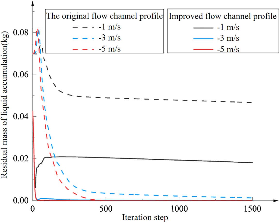
Figure 21: Residual liquid mass convergence curves of different flow channel profiles

Table 10 presents a summary of CFD-calculated residual liquid mass for various flow channel profile curves.

The initial liquid accumulation height is 17 mm, with the mass decreasing from 0.070 to 0.042 kg following the improvement of the flow channel profile at the valve body’s base. At a 1 m/s purge gas flow rate, the final purging efficiencies are 33.40% and 57.43% before and after the improvement, respectively. Under a 3 m/s purge gas flow rate, the efficiencies rise to 98.12% and 100%, respectively, post-improvement, suggesting that the critical purge flow rate falls below 3 m/s. These findings underscore the significant impact of the valve body’s base flow channel profile on residual liquid mass and the critical purge flow rate post-purging.

6  Conclusion

The numerical simulation method of anti-crystallization purging two-phase flow of molten salt regulating valve is studied, involving the selection of turbulence model and near-wall treatment, the selection of multiphase flow model, the application of dynamic grid adaptation, the establishment of molten salt regulating valve liquid accumulation model, and the convergence control of two-phase flow simulation. Based on the visual experiment and numerical simulation results in the literature, the accuracy of CFD gas-liquid two-phase flow simulation method for anti-crystallization purging of molten salt regulating valve is also verified. The numerical simulation of the DN50 PN50 conventional molten salt regulating valve body anti-crystallization purge reveals four distinct stages: the initial violent surge stage, the liquid discharge stage, the liquid partial fall stage, and the liquid dissipation stage. At an initial liquid accumulation height of 17 mm, the residual liquid mass as a percentage of the initial accumulation is 1.88% at a gas purge flow rate of 3 m/s and 0% at 5 m/s, indicating that the critical purge flow rate is greater than 3 m/s but less than 5 m/s.

At the same time, the following conclusions are drawn from the study of anti-crystallization purge gas-liquid two-phase flow under multiple working conditions:

1. The critical purge flow rate UC has nothing to do with the initial liquid volume.

2. When the purge gas flow rate falls below the critical purge flow rate, the residual liquid accumulation mass is proportional to the initial liquid accumulation amount. Beyond a certain point in time, the residual liquid accumulation mass remains largely unchanged with further increases in purge duration.

3. At purge gas flow rates exceeding the critical purge flow rate, the initial liquid accumulation mass has no influence on the mass of the residual liquid. Near the critical purge flow rate, the initial liquid accumulation mass exerts minimal impact on the mass of the remaining liquid.

4. As the purge gas flow rate increases, the liquid discharge becomes larger. When the purge gas flow rate exceeds the critical purge flow rate, the greater the purge gas flow rate, the shorter the time required for liquid emptying.

5. The profile of the flow channel at the bottom of the valve body has a significant effect on the residual liquid accumulation mass and the critical purge flow velocity.

According to the above research, the gas-liquid two-phase flow characteristics of anti-crystallization purging of molten salt regulating valve are obtained, providing a reference for the optimization of the anti-crystallization design of molten salt regulating valve.

Acknowledgement: We thank the other members of the Machinery Industry Pump and Special Valve Engineering Research Center, Lanzhou University of Technology team for their support of this study.

Funding Statement: The authors received no specific funding for this study.

Author Contributions: Shuxun Li made contributions through review, modification, amendment, supervision. Jianwei Wang was responsible for the design of the work plan, numerical simulation, data analysis, chart drawing, and article writing. Tingjin Ma performed data review and guidance. Guolong Deng conducted numerical simulation technical guidance and data analysis. Wei Li revised and supervised the article. All authors reviewed the results and approved the final version of the manuscript.

Availability of Data and Materials: The data that support the findings of this study are available from the corresponding author upon reasonable request.

Ethics Approval: Not applicable.

Conflicts of Interest: The authors declare no conflicts of interest to report regarding the present study.

References

1. Flamant G, Grange B, Wheeldon J, Siros F, Valentin B, Bataille F, et al. Opportunities and challenges in using particle circulation loops for concentrated solar power applications. Progress Energy Combust Sci. 2023;94:101056. [Google Scholar]

2. Zhang Q, Jiang K, Ge Z, Yang L, Du X. Control strategy of molten salt solar power tower plant function as peak load regulation in grid. Appl Energy. 2021;294:116967. [Google Scholar]

3. Roper R, Harkema M, Sabharwall P, Riddle C, Chisholm B, Day B, et al. Molten salt for advanced energy applications: a review. Ann Nuclear Energy. 2022;169:108924. [Google Scholar]

4. Bonk A, Sau S, Uranga N, Hernaiz M, Bauer T. Advanced heat transfer fluids for direct molten salt line-focusing CSP plants. Prog Energy Combust Sci. 2018;67:69–87. [Google Scholar]

5. Cheng W, Gu B, Shao C, Wang Y. Hydraulic characteristics of molten salt pump transporting solid-liquid two-phase medium. Nucl Eng Des. 2017;324:220–30. [Google Scholar]

6. Guo R, Zhang W, Jiang J, Liu Z. Numerical simulation of mobile pipeline gas-gap emptying based on OLGA. J Chem Eng Chin Univ. 2017;31(2):337–45. [Google Scholar]

7. Bissor E, Ullmann A, Brauner N. Liquid displacement from lower section of hilly-terrain natural gas pipelines. J Nat Gas Sci Eng. 2020;73:103046. doi:10.1016/j.jngse.2019.103046. [Google Scholar] [CrossRef]

8. Magnini M, Ullmann A, Brauner N, Thome J. Numerical study of water displacement from the elbow of an inclined oil pipeline. J Pet Sci Eng. 2018;166:1000–17. doi:10.1016/j.petrol.2018.03.067. [Google Scholar] [CrossRef]

9. Farouk M, El-Gamal M. CFD simulation of purging process for dead-ends in water intermittent distribution systems. Ain Shams Eng J. 2021;12(1):167–79. doi:10.1016/j.asej.2020.06.013. [Google Scholar] [CrossRef]

10. Sikora M, Anweiler S, Meyer J. Comprehensive analysis of two-phase liquid-gas flow structures in varied channel geometries and thermal environments. Int J Heat Mass Transf. 2024;228:125665. doi:10.1016/j.ijheatmasstransfer.2024.125665. [Google Scholar] [CrossRef]

11. Mondal P, Lahiri SK, Ghanta KC. Understanding two-phase flow behavior: CFD Assessment of silicone oil-air and water-air in an intermediate vertical pipe. Can J Chem Eng. 2024;102(12):4416–39. [Google Scholar]

12. Passoni S, Carraretto IM, Mereu R, Colombo LP. Two-phase stratified flow in horizontal pipes: a CFD study to improve prediction of pressure gradient and void fraction. Chem Eng Res Des. 2023;191:38–49. [Google Scholar]

13. Mondal A, Sharma SL. Modeling and simulation of air-water upward annular flow characteristics in a vertical tube using CFD. Nucl Eng Technol. 2024;56(7):2881–92. [Google Scholar]

14. Li S, Shen H, Liu B, Hu Y, Ma T. Pressure pulse response of high temperature molten salt check valve hit by crystal particles. J Shanghai Jiaotong Univ (Sci). 2024;29(2):271–9. [Google Scholar]

15. He X, Yu Y, Xie Z, Zhou Q. A modified CFD-DEM method for accurate prediction of the minimum fluidization velocity. Int J Fluid Eng. 2024;1(2):023902. [Google Scholar]

16. Gong J, Li G, Liu R, Wang Z. Numerical calculation of gas-liquid two-phase flow in tesla valve. Aerospace. 2024;11(5):409. [Google Scholar]

17. Prieto C, Fereres S, Ruiz-Cabañas FJ, Rodríguez-Sánchez A, Montero C. Carbonate molten salt solar thermal pilot facility: plant design, commissioning and operation up to 700°C. Renew Energy. 2020;151:528–41. [Google Scholar]

18. Yang H. Research on concentrating model and optimal scheduling system of heliostat (Master’s Thesis). Xi’an University of Technology: Xi’an, China; 2023. [Google Scholar]

19. Dong X, Zhang S, Zhang Y, Liu L. Experimental investigation on heat transfer characteristic of molten salt flow across vapor-liquid two-phase flow in tube. Acta Energiae Solaris Sinica. 2023;44(7):241–7. [Google Scholar]

20. Zeng Y, Cui G, Wu W, Xu C, Huang J, Wang J, et al. Numerical simulation study on flow heat transfer and stress distribution of shell-and-tube superheater in molten salt solar thermal power station. Processes. 2022;10(5):1003. [Google Scholar]

21. Zhang Y. Study on preparation and heat storage mechanism of nitrate based nanocomposites (Ph.D. Thesis). University of Chinese Academy of Sciences (Qinghai Institute of Salt Lakes, Chinese Academy of SciencesQinghai, China; 2021. [Google Scholar]

22. Jin Y, Zhang D, Shi L, Shi W, Wang D. Effect of molten salt properties on internal flow and disk friction loss characteristics of molten salt pump. Acta Energiae Solaris Sinica. 2020;41(11):176–84. [Google Scholar]

23. ANSYS Inc. ANSYS fluent theory guide, release 17.2. Canonsburg, PA, USA: ANSYS Inc.; 2016. [Google Scholar]

24. Brackbill JU, Kothe DB, Zemach C. A continuum method for modeling surface tension. J Comput Phys. 1992;100(2):335–54. [Google Scholar]

25. Wang D, Cao L, Wang W, Hu J. A numerical study on the effect of the backflow hole position on the performances of a self-priming pump. Fluid Dyn Mater Proc. 2024;20(5):1103–22. doi:10.32604/fdmp.2023.042654. [Google Scholar] [CrossRef]

26. Shih TH, Liou WW, Shabbir A, Yang Z, Zhu J. A new k-ε eddy viscosity model for high Reynolds number turbulent flows. Comput Fluids. 1995;24(3):227–38. [Google Scholar]

27. Mondal P, Lahiri SK, Ghanta KC. Assessment of ansys-fluent code for computation of two-phase flow characteristics: a comparative study of water-air and silicone oil-air in a vertical pipe. J Fluid Eng. 2024;146(12):121403. [Google Scholar]

28. Jaeger J, Santos CM, Rosa LM, Meier HF, Noriler D. Experimental and numerical evaluation of slugs in a vertical air-water flow. Int J Multiphase Flow. 2018;101:152–66. [Google Scholar]

29. Akhlaghi M, Mohammadi V, Nouri NM, Taherkhani M, Karimi M. Multi-fluid VOF model assessment to simulate the horizontal air-water intermittent flow. Chem Eng Res Des. 2019;152:48–59. [Google Scholar]

30. Dong X, Hao C, Liu C. Correlation between vorticity, Liutex and shear in boundary layer transition. Comput Fluids. 2022;238:105371. [Google Scholar]

31. Yu Y, Shrestha P, Alvarez O, Nottage C, Liu C. Investigation of correlation between vorticity, Q, λci, λ2, Δ and Liutex. Comput Fluids. 2021;225:104977. [Google Scholar]