Modeling Oil Production and Heat Distribution during Hot Water-Flooding in an Oil Reservoir

1  Introduction

An oil reservoir is a porous rock which contains hydrocarbons and resides hundreds of meters underneath the ground. It is usually heterogeneous, meaning that their properties, such as porosity and permeability, vary in space.

At the early stage of oil exploration, the reservoir is at equilibrium pressure with the atmosphere. Any perturbation, such as a drill of a well into the reservoir, immediately disturbs the equilibrium pressure and this causes the hydrocarbons to flow out. This is usually termed the primary recovery technique. This process only leads to about 20% production of the total hydrocarbon initially present in the reservoir. To continue production, the secondary recovery method can be applied. This involves injecting water or gas at an injection well, which then pushes out the hydrocarbons at the production well. This process may also lead to the production of another 20% of the hydrocarbons. In order to further production, another approach called Tertiary recovery or enhanced oil recovery (EOR) can be employed. This involves the injection of some special substances like polymers, foam, or solvents. These injected substances can enhance the miscibility of oil and water, thus leading to improved production. The present study is focused on hot waterflooding. See by Ezekwe [1] and also Ursegov and Zakharian [2].

In both secondary and tertiary recovery techniques, it is obvious that the amount of water and oil components would vary across the reservoir-as one goes from the injection well to the production well. Hence, it would be of operational importance to know when water starts to be produced. Also, it is important to know the effects of the velocity of water injection, and even fluid properties, on the rate of production. The knowledge can be used by reservoir engineers to predict and optimize production, support decision marking, and access different operating conditions among others.

Consequently, much research attention has been paid to modeling and simulation of the dynamics of oil recovery processes, especially the secondary and tertiary recovery techniques. For example, finite element based simulations of oil reservoirs can be found in the book of Chavent and Jaffre [3], while finite volume based models are discussed by Aarnes et al. [4]; another classical book in the subject is the one by Aziz [5]. Esfe and co-authors [6] investigated the use of nanofluids in EOR; they considered SiO2,Al2O3 and CuO nonoparticles with water as the base fluid. Their results show that increasing the inlet temperature has effect on the EOR process. Zhao and Gates [7] used a stochastic optimization algorithm (simulated annealing) to investigate the effects of water temperature, injection pressure , and other reservoir conditions on the performance of hot water-flooding. The results show that starting with high injecting water temperature and ending with the low injecting temperature improves the performance of the hot water-flooding process, and so do high injecting pressure.

According to Dong et al. [8], the dissolution of carbon dioxide in the reservoir oil decrease the oil viscosity which favors the miscibility between oil and water. Also, the dissolved carbon dioxide cause the oil volume to expand which increases the relative permeability of oil. Hence, Marotto and Pires [9] mathematically investigated the use of carbonated water (carbon dioxide injected into hot water) in an EOR process. Their model involves three hyperbolic partial differential equations which were formulated under the assumption of two-phase, one-dimensional flow in a homogeneous reservoir without diffusion, chemical reaction, gravity, or capillary effects. They defined a constant, KD as the ratio of Henry’s constant of the carbon dioxide in the oil phase to Henry’s constant of the carbon dioxide in the water phase. Their results show that the increase in KD (transferring more carbon dioxide to the oil phase) leads to an increase in the recovery factor. Wang [10] presented a mathematical model of steam flooding and used a meshless weighted least squares method to approximate the time evolution of temperature and saturation of oil and water. The results show that porosity affects the distribution of gas saturation and the temperature. Masoomi and Torabi [11] presented numerical simulations to predict temperature distribution and performance of hot-water flooding in oil reservoirs. They found that the relative permeability of oil is sensitive to temperature change. They also carried out laboratory experiments and used it to validate the numerical results.

From the available literature, the following important issues have not be addressed to satisfaction, namely (i) incorporating real-data into viscosity models (via regression analysis) and using it in the model equations, (ii) adopting a combination of thermal conductivity to derive the thermal conductivity of the oil-water mixture and using it in the heat model, (iii) investigating the effects of injection velocity and/or temperature of the injected water on the oil production in the waterflooding process, and (iv) deriving a formula that links the water saturation to the percentage of oil production.

Consequently, this paper presents a study that begins with real experimental data and uses it to first develop viscosity models for oil and water. These are then used to develop models and simulations for predicting the rate of oil recovery during hot waterflooding in a reservoir containing Bonny-light hydrocarbon. The arrangement of the paper is as follows. In the introductory section, we begin by presenting the model equations for water saturation and heat evolution. These equations contain nonlinear fluxes which include the viscosity of oil and water and also their thermal conductivities. For this, in Sections 2.1 and 2.2, we use experimental data to propose new viscosity models for Bonny-light crude oil and water. In the numerical analysis Section 3, we propose a modified HLL numerical flux function and apply it to derive a hybrid numerical discretization comprising finite volume and finite difference methods on a staggered grid. The convergence of the proposed method is numerically verified. Simulations, investigations, and results are presented and discussed. Lastly, concluding remarks are made.

2  Mathematical Model of Water Saturation and Temperature during Hot Water-Flooding

In this section, we present the mathematical statement of the reservoir problems under study. We consider a horizontal one-dimensional oil reservoir with an injection well at the left end and a production well at the right end. At time zero, hot water starts to be injected into the reservoir from the injection well, our goal is to predict the water saturation and temperature of the oil-water fluid in the reservoir at later times. We make the following assumptions:

(i)   The reservoir is initially filled with 99% oil,

(ii)   Gravitational and capillary effects are neglected,

(iii)   The reservoir is assumed to be homogeneous,

(iv)   The relative permeability of water depends on the saturation of water, also the relative permeability of oil depends on the saturation of oil,

(v)   The viscosity of oil is dependent on the temperature, and the same is true for the viscosity of water,

(vi)   The hot water is injected at a constant rate, v and constant temperature, Twall.

Under these assumptions, the equation governing the time evolution of the water saturation sw(x,t) is given by the following Buckley-Leverrete partial differential equation:

∂sw∂t+vϕ∂f(sw,T)∂x=0.(1)

Here, v and ϕ are the fluid velocity and porosity, respectively, while f(sw,T) is the water fractional flow, and it measures the fraction of water in the total flow, and is defined as

f(sw,T)=λw(sw,T)λw(sw,T)+λo(sw,T),(2)

with

λw(sw,T)=krw(sw)μw(T)andλo(sw,T)=kro(so)μo(T)(3)

being the mobilities of water and oil phases, respectively. Also, krw and kro are the relative permeabilities of water and oil, while μw((T)) and μo(T) are their respective viscosities which depend on the temperature, T=T(x,t). Note so=1−sw is the oil saturation.

To write the fractional flow in closed form, we need to define the relative permeability functions and also the viscosity functions. Later, we will use real data obtained from the literature to construct models for viscosity dependence on temperature, but at the moment let us define the relative permeability functions. For this, we adopt the power law model according to Holden and Risebro [12] which states

krp(sp)=sp2,p=o,w.

With the above definition, the fractional flow function becomes

f(sw,T)=sw2sw2+μw(T)μo(T)(1−sw)2.(4)

Hence, the water saturation is governed by the Buckley-Leverett Eq. (1) with saturation- and temperature-dependent fractional flow (4).

The Temperature Model

To derive the temperature of the fluid, we assume that no heat is generated or lost within the reservoir. The only heat source is the one that comes from the injected hot water from the injection well. We require that the thermal conductivity (κow) of the oil-water fluid must reduce to the thermal conductivity of oil alone (κo) if water is totally absent, but if oil is completely absent, then it must reduce to the thermal conductivity (κw) of water. To realize this requirement, we propose the following model:

κow=swκw+(1−sw)κo.(5)

Observe that this model satisfies the requirement above. Even in the case of temperature-dependent thermal conductivity, we can just define

κow(sw,T)=swκw(T)+(1−sw)κo(T).(6)

With the above information, we propose the following heat model:

∂T∂t+v∂T∂x=∂∂x((swκw(T)+(1−sw)κo(T))∂T∂x).(7)

This Eq. (7) is the one that governs the temperature of the mixture of oil and water in the reservoir. In this work, we shall assume that the thermal conductivity of both oil and water are constant. Next, we find expressions for the oil and water viscosities as a function of temperature.

2.1 Oil Viscosity as a Function of Temperature

Our goal here is to derive the oil viscosity function μo(T) which appear in the saturation model. To do this, we will use the experimental data presented by Abdulkareem and Kovo [13] for viscosity and temperature of hydrocarbons in the different reservoirs in the Niger Delta of Nigeria. A similar study is conducted by Isehunwa and colleagues [14]. The approach we adopt here is to use different regression and curve fitting packages available in Python. The data is the Bonny-light data extracted from Table 1 in [13]; a scatter plot of the experimental data and its predicted data from the model proposed in [13] are shown in Fig. 1. Unfortunately, the actual parameter values obtained in [13] for the regression model are not listed in their paper, hence we cannot use their model. Also, an analysis of their model reveals that better models can be derived. Hence, we propose other new models in the present paper. This will allow us to select the model that best fits the data.

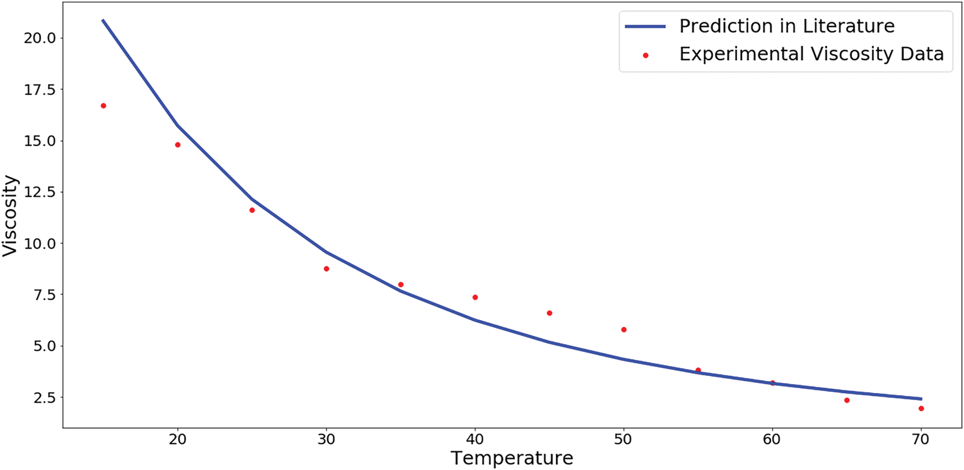
Figure 1: Plot of viscosity of bonny-light crude oil. Data source: Table 1 in [13]

From the scatter plot, we can see a form of exponential decay, hence we propose the following models:

μ(T)=a0e−a1T, (Viscosity-Model 1)(8)

μ(T)=b0exp(b11+T−37.78310.93), (Viscosity-Model 2)(9)

log⁡μ(T)=p0+p1T, (Viscosity-Model 3)(10)

where a0,a1,b1,b2,p0,p2 are model parameters to be determined using the experimental data. The second model (9) is based on taking the exponential of the model adopted in [13] with s=1. By using the scipy.optimize.curve_fit and numpy.polyfit functions in Python, we obtain the following resultsa0=28.74425361,a1=0.03560651,b0=0.00015388,b1=10.769714796,p0=−0.038074809,p1=3.44098224. To select the best model among all the models, we plot their results in Fig. 2 and also compute the mean square errors (MSE) given by

MSE=1N(∑i=1N(yi−yi,predicted)2)(11)

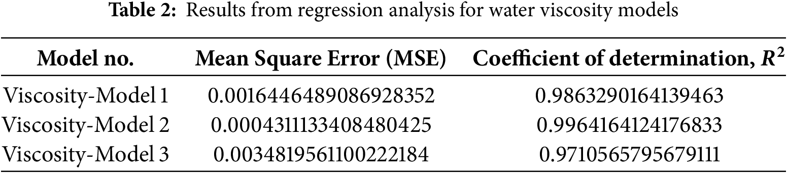
and also the coefficient of determination, R2

R2=1−∑i=1N(yi−yi,predicted)2∑i=1N(yi−y¯)2,(12)

where yi,yi,predicted are the i-th experimental and predicted values and y¯ is the mean of the experimental values, y¯=1N∑i=1Nyi, and N is the number of data points. These values are shown in Table 1.

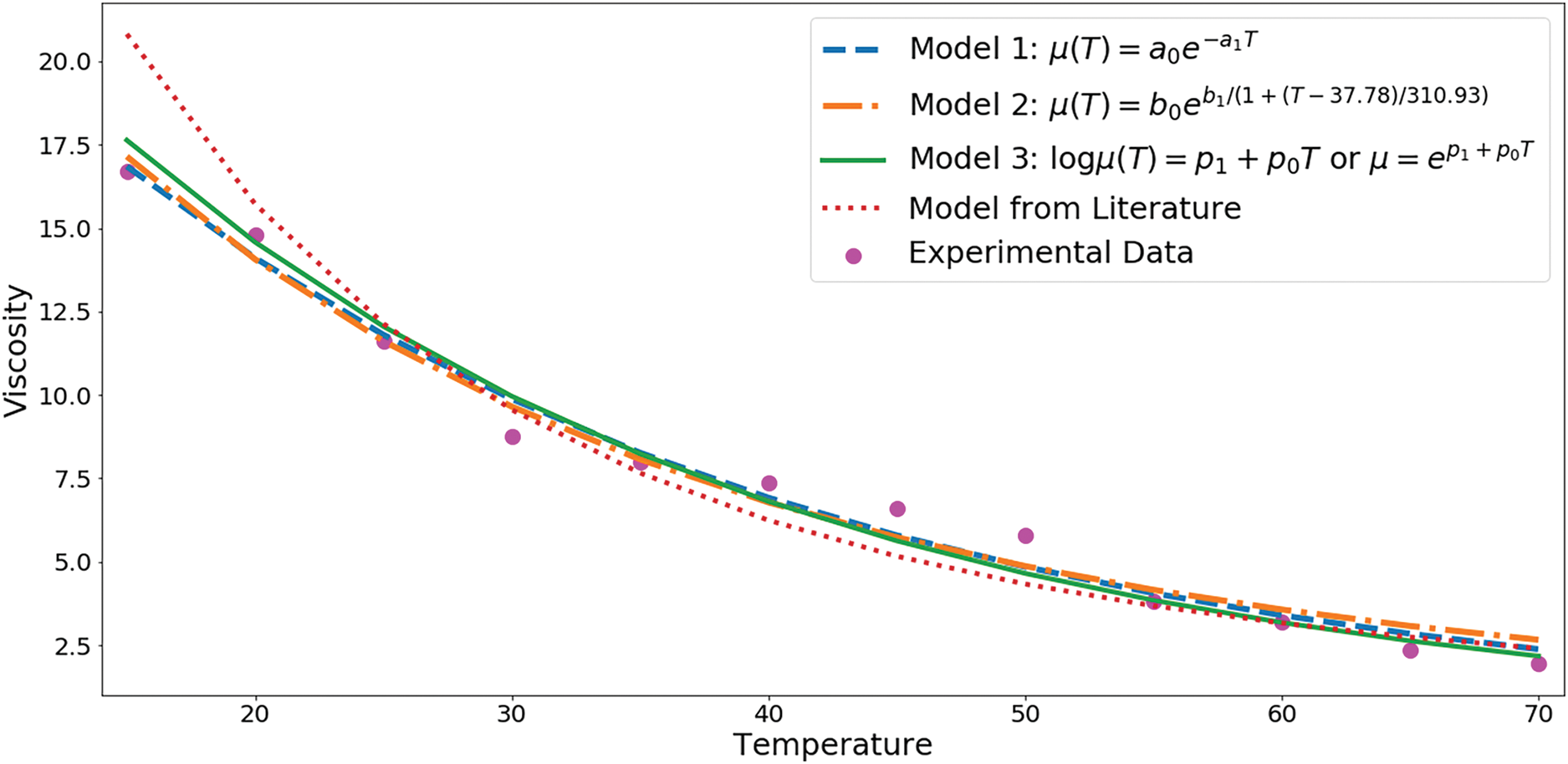
Figure 2: Plot of predictions of the suggested models for bonny-light oil viscosity

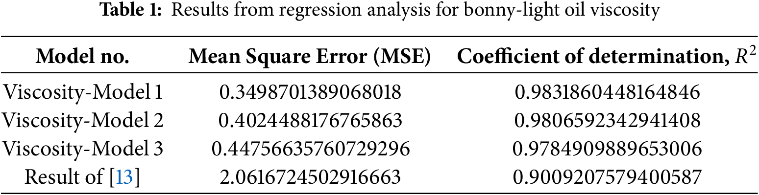
From Table 1 we see that the first model has the least MSE and also the highest R2 score, hence we select it as our oil viscosity model in this work. Therefore, the oil viscosity function needed in the saturation model (1) is defined as

μo(T)=28.74425361e−0.03560651T.(13)

2.2 Water Viscosity as a Function of Temperature

Similar to the oil viscosity model above, we also develop a model for the water viscosity in this subsection. We use the data provided for water viscosity versus temperature in the webpage https://wiki.anton-paar.com/en/water/ (accessed on 20 January 2025), and also apply the three regression models given in (8)–(10). This gives the following parameters: a0=1.66265383,   a1=0.02361327,   b0=0.000824731734, b1=6.71358077,p0=−0.0203676,p1=0.43725832. The predictions of each model is plotted in Fig. 3 and the relevant statistical measures are tabulated in Table 2. The results show that the second model, namely

μw(T)=0.000824731734exp(6.713580771+T−37.78310.93),(14)

has the smallest MSE and the best R2 value, hence is selected as the model for water viscosity as a function of temperature.

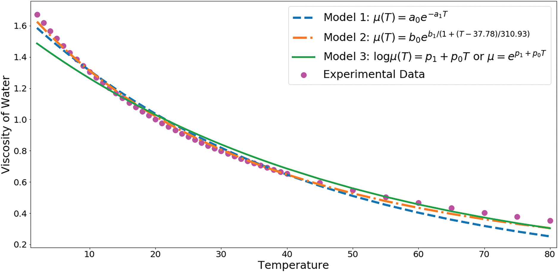
Figure 3: Plot of predictions of the three models for viscosity of water

As seen above, model 1 performed best for the oil viscosity, while model 2 performed best for the water viscosity. Therefore, one important lesson from the above analyses is that no one model is best for all situations. A better model for one problem might be poor for another problem. This concludes the modeling of the viscosity functions. Finally, we state the boundary and initial conditions for the models (1) and (7).

2.3 Boundary and Initial Conditions

The injection well will be maintained at water saturation of one and the temperature will be equal to the injecting water temperature, Twall, while the production well will attain whatever water saturation and temperature that are produced from inside the reservoir. To model these, we adopt non-homogeneous Dirichlet boundary conditions at the injection well and homogeneous Neumann boundary conditions at the production well, namely

sw(0,t)=1,T(0,t)=Twall for all t≥0,∂T∂x|x=xR=0,∂sw∂x|x=xR=0, for all t≥0.(15)

At the initial time, we assume that the reservoir is completely filled with oil while the injection well is completely filled with water. Also, we assume that, at the initial time, the temperature is Twall at the injection well and rapidly decreases to zero after the injection well. Hence,

sw(x,0)={1 if x≤0.01,0 otherwise.T(x,0)=Twalle−200x.(16)

2.4 Summary of the Reservoir Model

The complete reservoir problem is governed by the saturation and heat equations (1) and (7) along with the fractional flow Eq. (4), the viscosity model (13), the boundary conditions (15) and the initial conditions (16). The above model is nonlinear, hence, does not have a closed form analytical solution. So, we propose a numerical method for it in the next section.

3  The Proposed Numerical Scheme

In this section, we construct the numerical algorithm to approximate the solution of the model proposed in Section 2. Since the saturation model (1) is hyperbolic whilst the temperature Eq. (7) is parabolic, we propose to use a finite volume method for the saturation model and a finite difference scheme for the temperature equation. In order to properly couple the two numerical schemes and avoid unnecessary approximations that may reduce the overall accuracy of the algorithm, we shall solve these problems in a staggered grid such that the saturation is computed at cell centres whilst the temperature is computed at the cell faces.

3.1 Staggered Grid Generation

Let [a,b] be divided into Ncell, (1<Ncell∈Z+) cells (sub-intervals). Define

h=b−aNcell,

so that the grid points are faces of the cells at the points xi=a+ih for i=0,1,⋯,Ncell≡Ii with cells, Ii=[xi,xi+1] centered at xi+1/2=xi+0.5h. We seek the solution of the saturation equation at the cell centers, xi+1/2 and that of the temperature equation at the faces xi.

Important Notation

At time tn, we denote si+1/2n as the approximation of the cell average of the saturation in the cell centered at xi+1/2, and Tin is the approximation of the temperature at the cell face at xi.

3.2 Finite Volume Scheme for the Saturation Equation

Let us define the following auxiliary functions:

F(sw,T)=vϕf(sw,T).

This is the physical flux function of the saturation Eq. (1), hence we can define an equivalent HLL numerical flux function for the saturation equation as

ℱ(wL,wR,TLR):={F(wL,TLR), if sL≥0,sRF(wL,TLR)−sLF(wR,TLR)+sLsR(wR−wL)sR−sL, if sL≤0≤sR,F(wR,TLR), if sR≤0,(17)

where the wave speeds are given Bouchut [15], see also Nwaigwe and Mungkasi [16] as

sL=mink{λk(wL,TLR),λk(wR,TLR)},sR=maxk{λk(wL,TLR),λk(wR,TLR)},(18)

where λk(wL,TLR),k=1,…,M, is the k-th eigenvalues computed with cell average saturation, wL and interface temperature, TLR. The physical eigenvalues are defined as

λ(sw,T)=2μw(T)μo(T)(1−sw)swvϕ(sw2+μw(T)μo(T)(1−sw))2.

With these, we propose the following finite volume scheme for the saturation equation:

si+1/2n+1=si+1/2n−Δth(ℱ(si+1/2n,si+3/2n,Ti+1n)−ℱ(si−1/2n,si+1/2n,Tin)).(19)

The boundary condition at the production well is

∂sn+1∂x|x=xNcell=0 or sNcell+1/2n+1=sNcell−1/2n+1.(20)

3.3 Finite Difference Scheme for the Temperature Equation

Define the discrete quantities

κj+1/2n=κ(sj+1/2n).

By using central discretization of the diffusion term, upwind treatment of the convection term and implicit time integration, we propose the following scheme for the heat equation:

Tin+1=Tin−vΔth(Tin+1−Ti−1n+1)+Δth2[κ(si+1/2n+1)(Ti+1n+1−Tin+1)−κ(si−1/2n+1)(Tin+1−Ti−1n+1)],i=0,1,⋯,Ncell.(21)

The boundary condition:

∂Tn+1∂x|x=xNcell=0 or TNcell+1n+1=TNcell−1n+1.(22)

3.4 Summary of the Numerical Scheme

The complete numerical scheme is as follows:

{si+1/2n+1=si+1/2n−Δth(ℱ(si+1/2n,si+3/2n,Ti+1n)−ℱ(si−1/2n,si+1/2n,Tin)),i=1,2,⋯,Ncell−2.si+1/2n+1=si+1/2n−Δth(ℱ(si+1/2n,si+1/2n,Ti+1n)−ℱ(si−1/2n,si+1/2n,Tin)),i=Ncell−1.Tin+1=Tin−vΔth(Tin+1−Ti−1n+1)+Δth2[κi−1/2n+1(Ti+1n+1−Tin+1)− κ(si−1/2n+1)(Tin+1−Ti−1n+1)],i=1,2,⋯,Ncell−1,Tin+1=Tin−vΔth(Tin+1−Ti−1n+1)+2Δth2κi−1/2n+1[Ti−1n+1−Tin+1],i=Ncell,(23)

This completes the numerical formulation of the problem.

4  Numerical Examples for Convergence

Convergence Analysis

The convergence of the first order finite volume scheme for conservation laws has been demonstrated in many books by LeVeque [17,18], also the convergence of the finite difference scheme has also been proved and numerically demonstrated in many papers, such as those by Nwaigwe and coworkers [19,20]. Therefore, we will skip the theoretical proof of the convergence of the schemes (23), instead we refer the reader to the above-mentioned sources. In this section, we provide an example and use it to numerically demonstrate that indeed, the proposed numerical scheme actually converges to the exact solution of the model (1) and (7). To this end, we consider the following modification of our proposed model. If we add an artificial source term, G(x,t), given by

G(x,t)=−2κwte−1t+1+40κwxe−10x−100κw(x−1)2e−10x−42κwe−10x+2tvxe−1t+1−2tve−1t+1+t(x−1)2e−1t+1(t+1)2−10vx2e−10x+22vxe−10x−12ve−10x+(x−1)2e−1t+1.(24)

to the right hand side of the temperature model (7). Then, set the initial conditions

sw(x,0)=1,T(x,0)=(x−1)2e−10x,(25)

the left boundary condition

T(0,t)=1+te−1/(1+t),(26)

and zero Neumann boundary conditions on the right side for both sw and T, then the exact solution for the model is given by

s(x,t)=1,T(x,t)=(x−1)2(e−10x+te−1/(1+t)).(27)

Hence, the system consisting of Eqs. (1), (7) and (24)–(26) (with G(x,t) added to the right side of (7)), has the exact solution given in (27). We use this to demonstrate that the proposed numerical method actually converges to the exact solution.

We apply the proposed numerical scheme to the above problem by using 200 equally spaced grid points in [0, 1]. The source term G(x,t) is discretized implicitly (since it does not involve an unknown) and we use the following parameters: v=0.05,ϕ=0.3,κw=0.5,κ0=0.5. The results are computed with a time step size of 1.25×10−5 and the computed numerical solution is outputted and compared with the exact solution at different times. These are shown in Figs. 4 and 5 for the temperature and saturation respectively. It can be seen that the numerical solution agrees with the exact solution at all times and for both temperature and water saturation. This gives us the confidence that our numerical scheme is actually correct and convergent and can be used to conduct our desired simulations. In the next section, we use the code to investigate the effect of various parameters on the system.

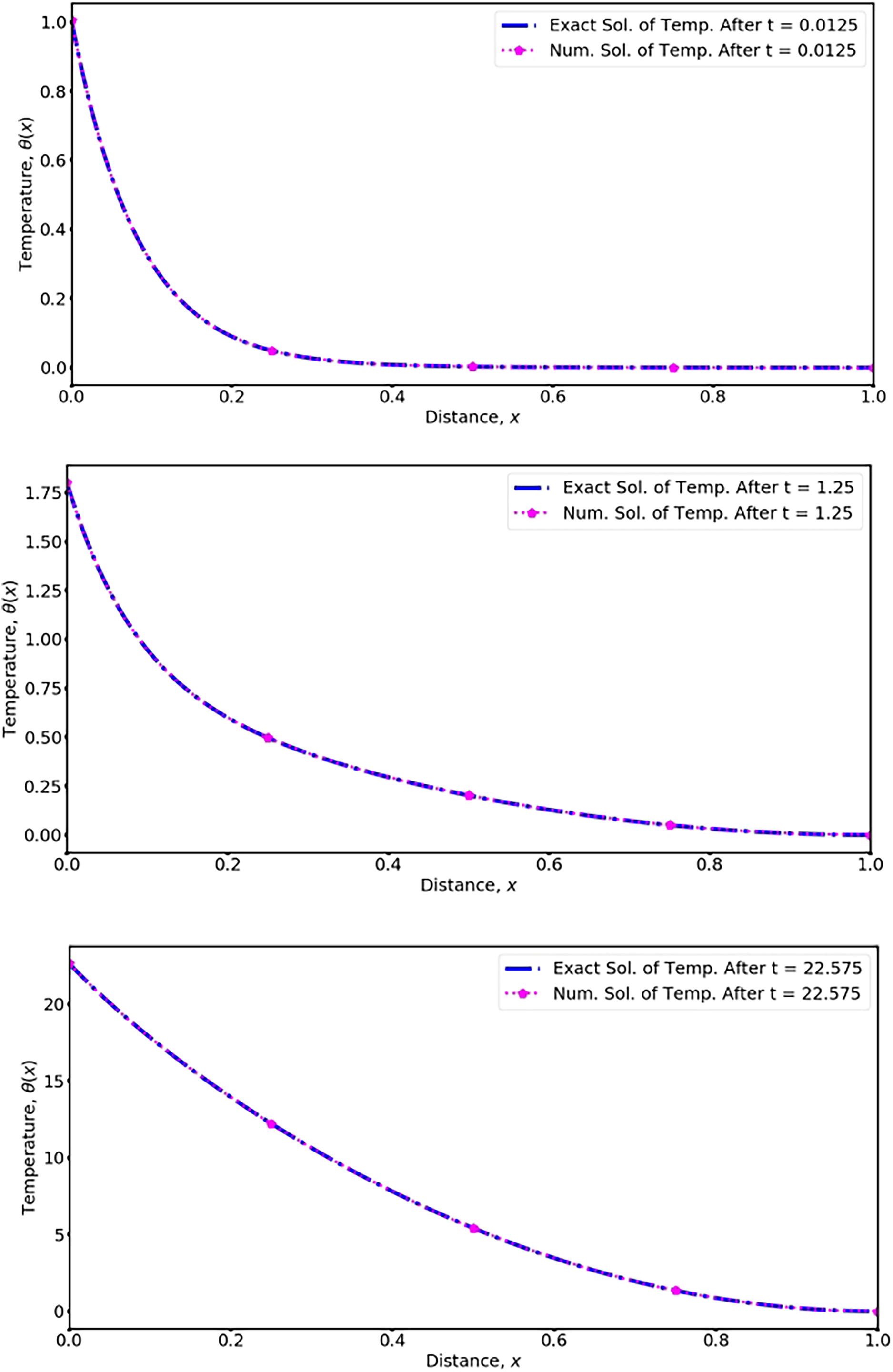
Figure 4: Comparison of exact and numerical solution of temperature for the test problem

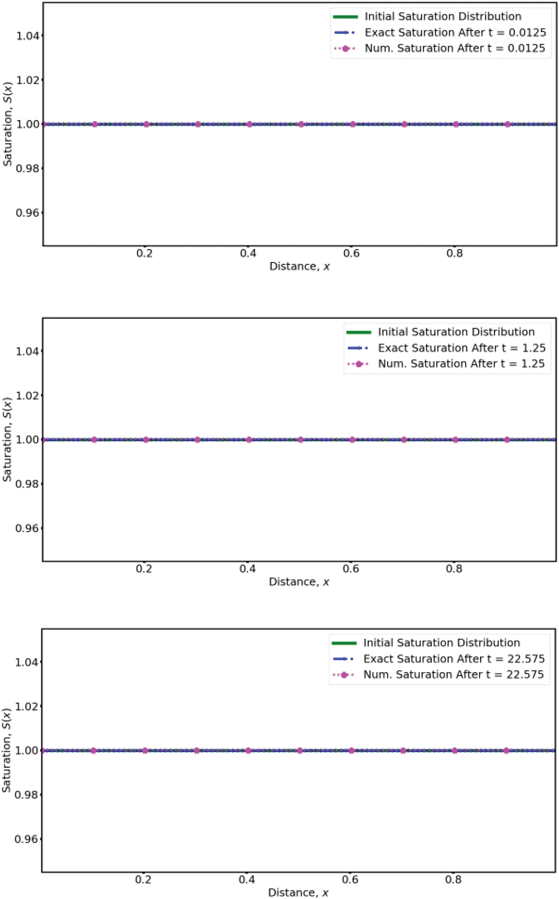
Figure 5: Comparison of exact and numerical solution of water saturation for the test problem

5  Numerical Simulations and Main Results

This section presents simulations to understand and predict the reservoir system. In particular, we present simulations to understand how the injection velocity and the temperature of the injected water affect oil production.

A measure of the percentage of oil recovered

We shall indicate the measure of oil production at any given time by calculating the total oil saturation (So,wn) remaining inside the reservoir at the given time, t=tn. Specifically, we first plot the water saturation against the distance (measured from the injection well towards the production well). Then, the area under this water saturation curve divided by the total area will be the total water saturation (ST,wn), and the total oil saturation shall be

ST,on=1−ST,wn.

To be able to know the percentage of oil that has been produced since exploration (start of simulation), we also need to know the initial amount of oil in the reservoir, which we also measure by using the term initial total oil saturation, denoted by ST,o0 and defined by

Initial Total Oil Saturation, ST,o0=1− Initial Total Water Saturation=1−h∑i=0Ncell−1sw(xi+1/2,0)=0.99.(28)

Here, sw(x,0) is the initial condition of water saturation defined in (16), while xi+1/2, the midpoints of the finite volume cells, and h are defined in Section 3. Note that the value, 0.99, would be different for different initial conditions. The number 0.99 means that the reservoir is 99% initially filled with oil, and our goal is to track(predict) how this value changes with time, and how it’s affected by the values of the injection velocity and wall temperature. Note, also, that the above formula is a discrete version of the continuous (exact) formula:

ST,o0=1−∫01sw(x,0)dx=1−0.01=0.99.

Moreover, we also use the midpoint rule to calculate the total water saturation, namely

ST,wn=∑i=0Ncell−1hsi+1/2n.(29)

This Eq. (29) is adopted since si+1/2n is the average of the water saturation in the grid cell centered at x=xi+1/2, which is the finite volume method.

Data

The following injected water temperature, Twall (in °C) values shall be considered 0.0,25.0,55.0,70.0,100.0,120.0, while the following injection velocity values, v are considered 0.0,0.05,0.2,0.25,0.35,0.5,1.0,1.5,2. The following initial temperature profile is considered:

T(x,0)=Twalle−200x,x∈[0,1],(30)

where Twall is varied with the various injection temperature values above. We shall examine the effects of Twall and v on the oil production. The simulation is conducted with 200 grid cells, time step size of 2.5×10−5 and run until t=5.

5.1 Results

The main goal of this subsection is to discuss how v and Twall affect the reservoir temperature, water saturation, and percentage of oil recovered. But before then let us first examine if our proposed model and numerical scheme actually respects the no motion effect when v=Twall=0.

5.1.1 Results under No Flux (v=0) and Zero Operating Temperature Twall=0

Let us start by presenting the results when v=0 and Twall=0. This means that the injected water is not hot, but cold (zero temperature). Hence, we must expect the reservoir to remain at zero temperature at all times since no heat is generated inside it. Fig. 6 shows the numerical solution of our model. One can see that the temperature remains at the initial zero temperature at all times as expected. Also, from the physical point of view, setting v=0 means no flux, and there would be no waterflooding, hence the initial saturation of water and oil would remain unchanged at all times. Fig. 7 shows our numerical experiment under this condition. It is also seen that the initial saturation profile remains unchanged over time. These results show that our model obeys fundamental physical processes, making it reliable.

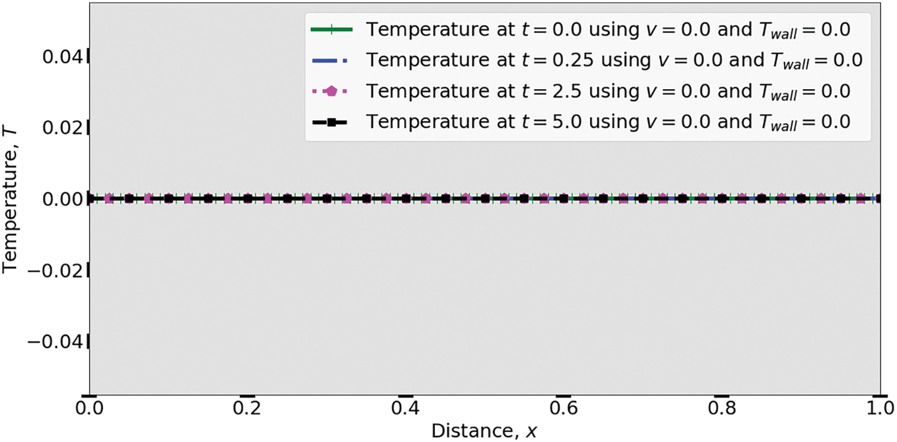
Figure 6: Temperature profiles at different times when v=Twall=0

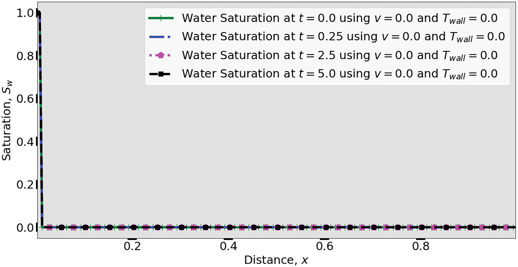
Figure 7: Water saturation at different times when v=Twall=0

5.1.2 Effects of Injection Velocity v on Temperature

The effects of the injection velocity on the reservoir temperature are shown in Fig. 8. The upper figure is the results at t=2.5, while the lower figure is at t=5. Both numerical experiments are conducted while setting the wall temperature (injecting water temperature) at a constant value of Twall=10oC. The results show that increasing the rate v at what the hot water is being injected at the injection well leads to an increase in the temperature of the fluid in the reservoir. The results are physically expected since a higher rate of hot water injection would increase the convection transport and also enhance the diffusive transport of heat, thereby increasing the temperature. Hence, these results are physically valid.

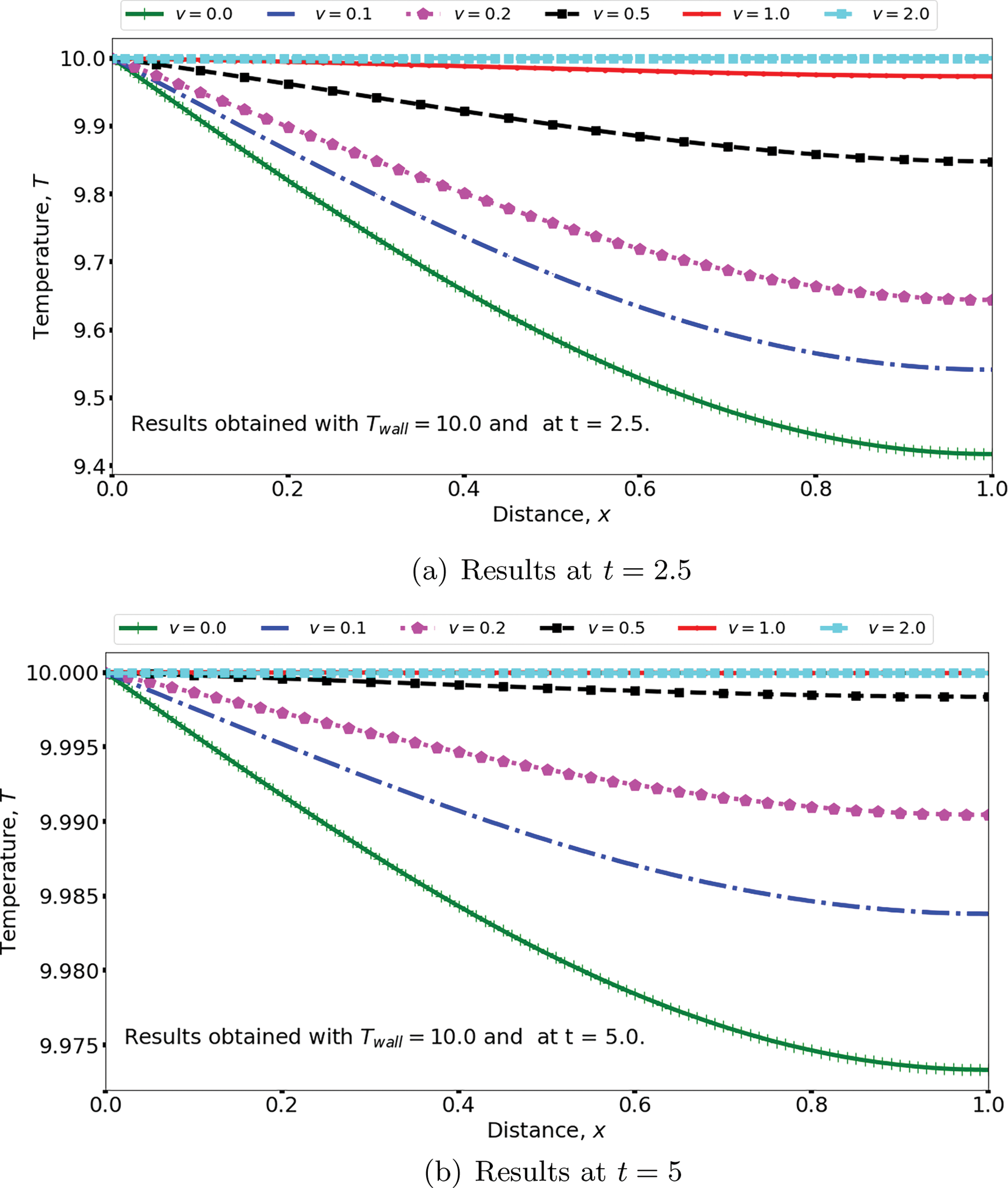
Figure 8: Effect of injection velocity on the temperature profiles

Also, notice that the temperature profiles in the lower figure (at t=5) are higher than those of the upper figure (t=2.5) for each velocity value. This shows that the temperature increases with time. This is also valid since more hot water is constantly being introduced into the initially cold reservoir.

5.1.3 Effects of Injection Velocity v on Water Saturation and Oil Production

Fig. 9 shows the plots of water saturation for different injection velocities at (a) t=0.25 and (b) t=5. First, we observe that the water saturation increases at all points with an increase in the injection velocity. This is the case at both t=0.25 and t=5. So, the water saturation increases with injection velocity. It is also seen that for a given value of the injection velocity v, the saturation is higher at t=5 than at t=0.25, meaning that the water saturation increases with time, which makes sense since water is continuously injected into the reservoir. Again, we also notice that for v=0, the water saturation remains at it’s initial condition (the green line) at both t=0.25 and t=5. This is consistent with our earlier result that shows that no velocity means no flooding in Section 5.1.1, see Fig. 7.

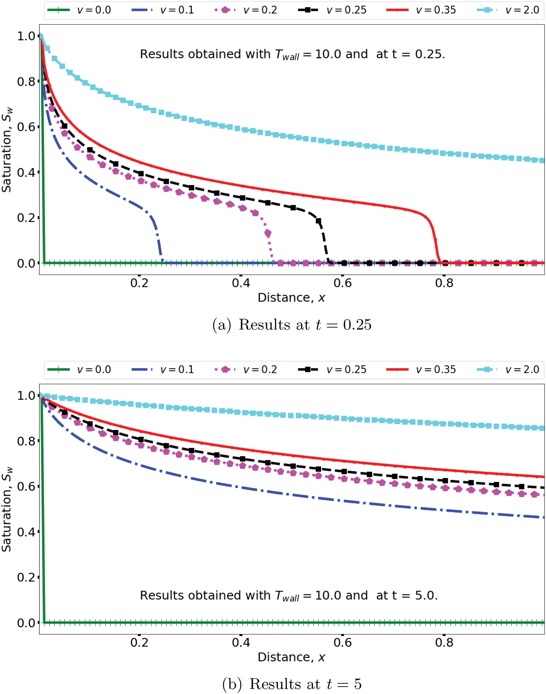
Figure 9: Effects of injection velocity on the water saturation

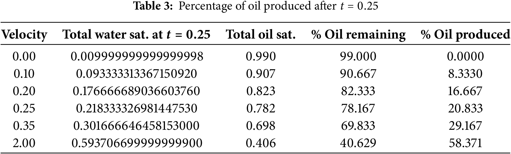
In order to relate the above observations to oil production and quantify the rate of production, we use the results in Fig. 9 to compute some important quantities which are Tabulated in Tables 3 and 4. As noted earlier, the reservoir is initially 99% filled with oil, see (28). Table 3 shows that at t=0.25, an injection velocity of zero leads to zero oil production (consistent with earlier results and physical reality), while an injection velocity of 0.1,0.2,0.25,0.35,2.0 leads to oil production at 8.3%,16.67%,20.8%,29.2% and 58.37%, respectively. This shows that the higher the injection velocity, the more oil is produced. Similarly, Table 4 shows that at t=5 the oil production rates for injection velocities of 0.1,0.2,0.25,0.35,2.0 are 58.97%,68%,70.8%,74.9% and 90.7%, respectively. Comparing these results in Table 4 with those of Table 3, we conclude that more oil is produced as time progresses.

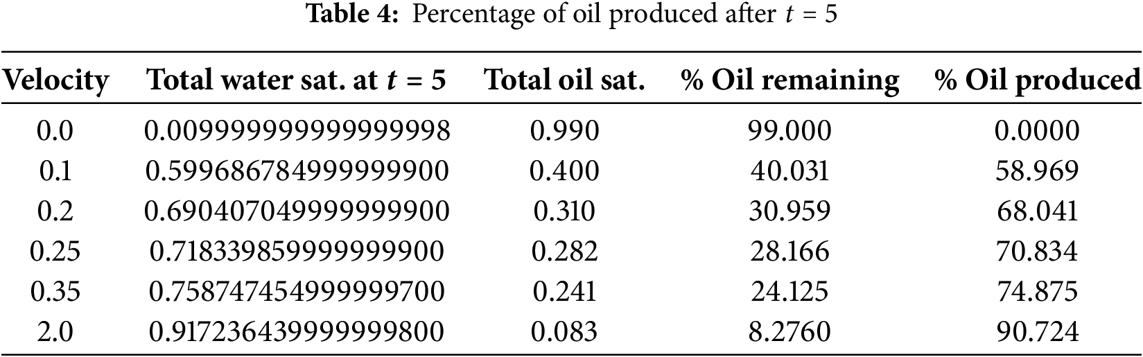
5.1.4 Effects of Wall Temperature Twall on Temperature

Even without simulation, it is common sense knowledge that an increase in the temperature of the injected water (the wall temperature) will lead to an increase in the temperature of the entire reservoir system. To demonstrate the consistency of our results with this physical reality, Fig. 10 shows our computed temperature distributions using different values of the wall temperature and at different times. Obviously, the temperature profiles are higher for higher wall temperatures and at all times. This particular result, again, establishes that our model obeys physical realities.

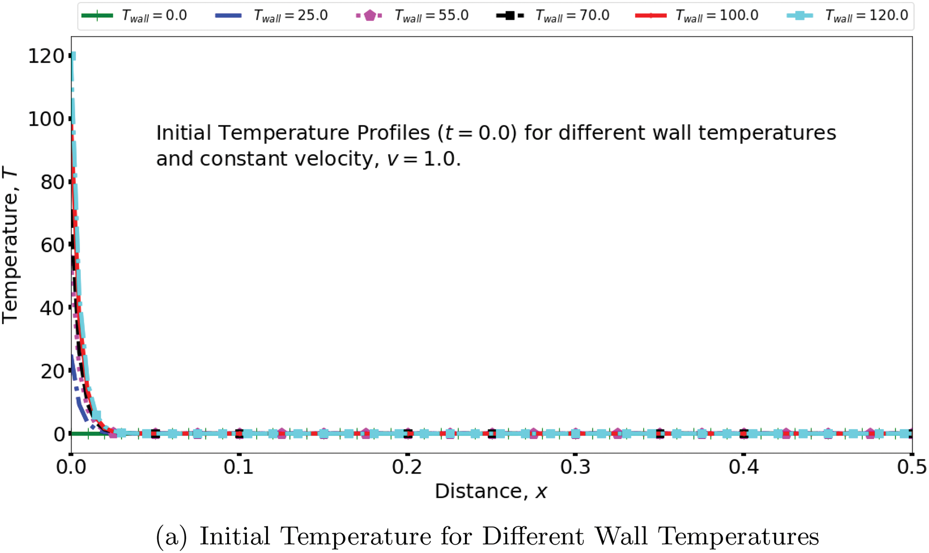
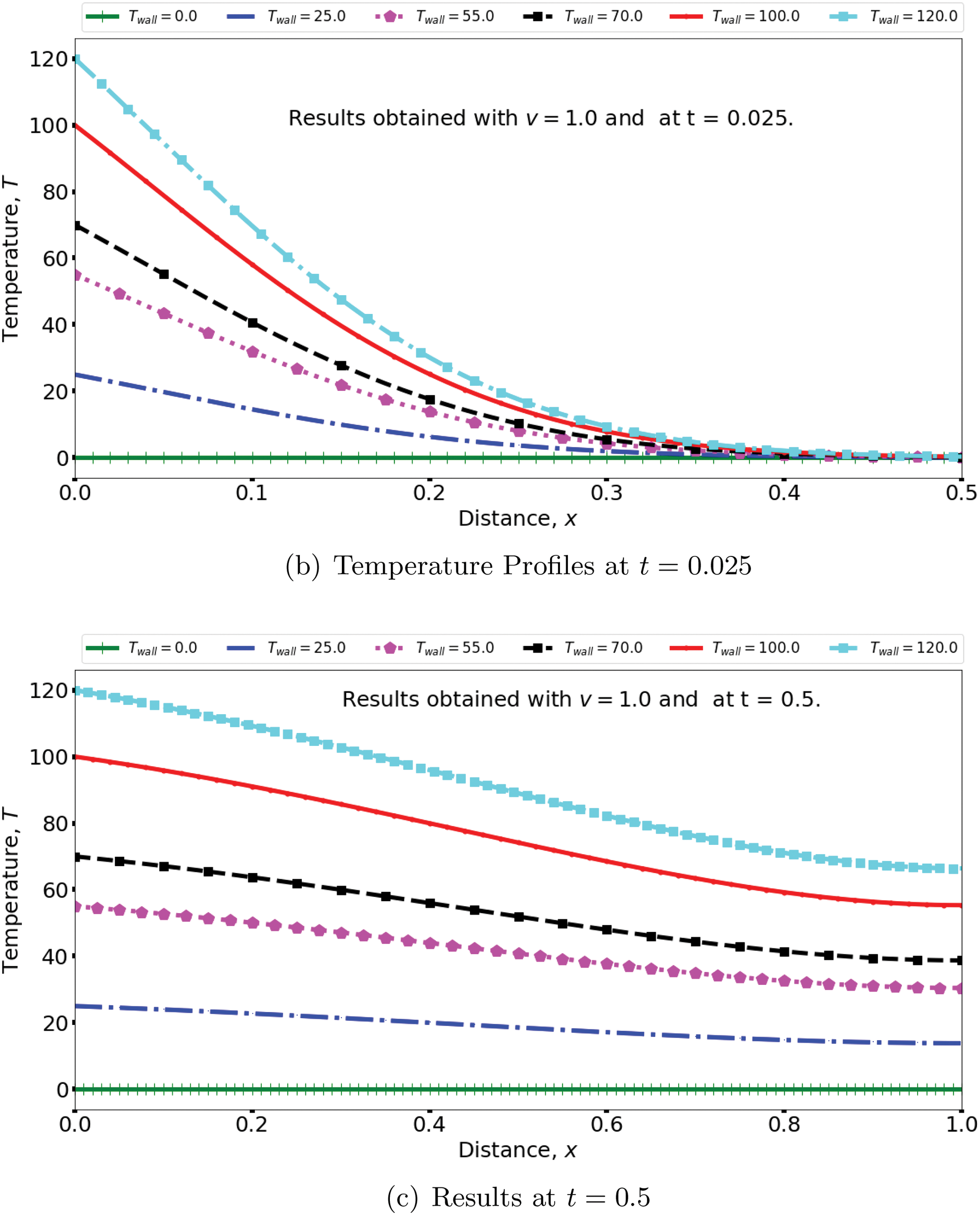
Figure 10: Effect of temperature of injected water (wall temperature, Twall) on the reservoir temperature distribution

5.1.5 Effects of Wall Temperature Twall on Water Saturation and Oil Production

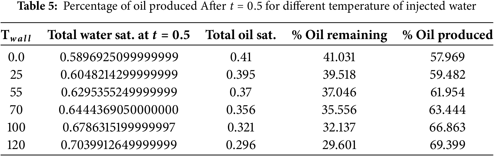
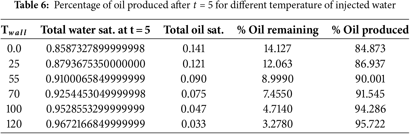
In Fig. 11, the plots of the water saturation for different wall temperatures (injected water temperature) are shown at (a) t=0.5 and (b) t=5. The results show that the saturation increases at all point in the reservoir as the wall temperature increases. This is the case for both t=0.5 and t=5. Note that the injection velocity used for these experiments is v=1. Therefore, even for Twall=0 the water saturation does not remain at the initial condition but flows with the nonzero velocity, v=1. Fig. 11a,b also shows that the water saturation increases with time.

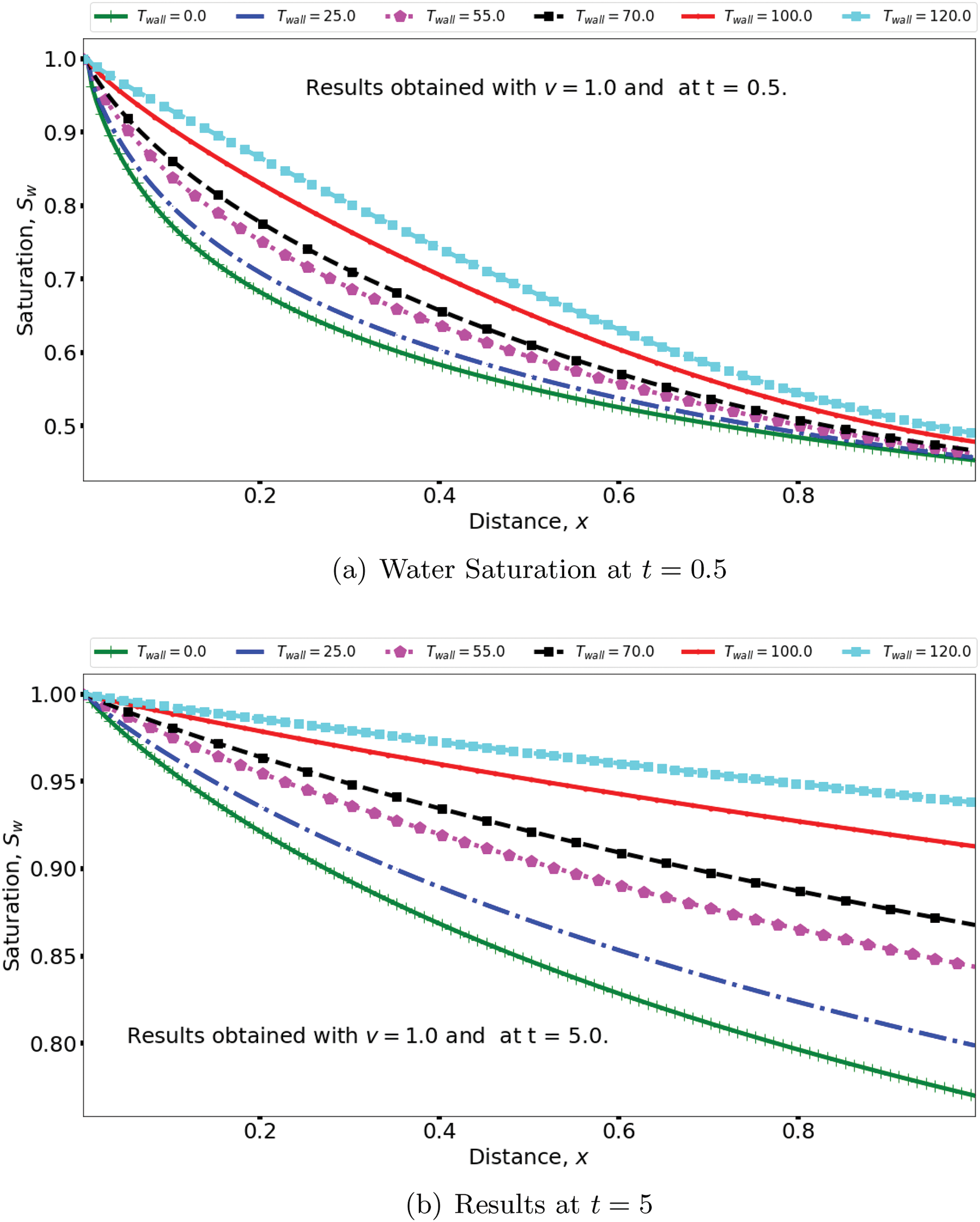
Figure 11: Effects of temperature of injected water on the water saturation and oil production

To quantify the rate of oil production, important quantities are computed and Tabulated in Tables 5 and 6. Table 5 shows that at t=0.5, the injected hot water at the temperature (in °C) of 0,25,55,70,100 and 120 led to oil production at 57.97%,59.48%,61.95%,63.44%,66.86% and 69.4%, respectively. Table 6 shows a repeat of the same trend in Table 5, moreover, the results also show that oil production increases with time.

6  Conclusion

In this paper, the mathematical and numerical modeling of the water saturation and heat distribution in a horizontal reservoir is conducted with the aim of predicting the rate or percentage of oil recovery in a hot water flooding process. To achieve this, the Bonny-light crude oil is chosen as a case study, and available experimental data found in the literature was used to conduct regression analyses to derive two temperature-dependent viscosity models for oil and water. Then a modified Buckley-Leverette model containing temperature-dependent nonlinear flux, and a convection-diffusion equation containing a convex combination as thermal conductivity are adopted for water saturation and temperature models. Finite volume and finite difference methods are formulated on a staggered grid to approximate the models. The following are the results found from the study:

(i)   No single regression model is fit for all viscosity problems, in particular the best regression model for oil viscosity is different from the one for the water viscosity,

(ii)   At wall (in-let) temperature of 10oC, increase in the injection velocity from 0.1 to 0.25 changed the rate of oil production from 8.33% to 20.8%,

(iii)   At injection velocity of v=1, an increase in the temperature of the injected water from 25oC to 55oC changed the production rate from 59.48% to 61.95%,

(iv)   Both high injection water temperature and high injection velocity are beneficial to high oil production,

(v)   Oil recovery is directly dependent on maintaining non-zero positive injection velocity.

Acknowledgement: The authors sincerely thank all the reviewers for their great suggestions which enormously improved this work. We also thank the editor for the efforts.

Funding Statement: The authors received no specific funding for this study.

Author Contributions: The authors confirm contributions to the paper as follows: study conception and design: Chinedu Nwaigwe; data collection: Chinedu Nwaigwe, Abdon Atangana; analysis and interpretation of results: Chinedu Nwaigwe, Abdon Atangana; software and code development: Chinedu Nwaigwe; literature: Chinedu Nwaigwe, Abdon Atangana; draft manuscript preparation: Chinedu Nwaigwe, Abdon Atangana. All authors reviewed the results and approved the final version of the manuscript.

Availability of Data and Materials: The datasets generated and analyzed during the current study are available from the corresponding author on reasonable request.

Ethics Approval: Not applicable.

Conflicts of Interest: The authors declare no conflicts of interest to report regarding the present study.

Nomenclature

References

1. Ezekwe N. Petroleum reservoir engineering practice. United States: Pearson Education; 2010. [Google Scholar]

2. Ursegov S, Zakharian A. Adaptive approach to petroleum reservoir simulation. Switzerland: Springer; 2021. [Google Scholar]

3. Brezzi F, Chavent G, Jaffre J. Mathematical models and finite elements for reservoir simulation: single phase, multiphase and multicomponent flows through porous media. Math Comput. 1988;50(182):640. doi:10.1016/s0168-2024(08)x7007-9. [Google Scholar] [CrossRef]

4. Aarnes JE, Gimse T, Lie KA. An introduction to the numerics of flow in porous media using matlab. In: Geometric modelling, numerical simulation, and optimization: applied mathematics at SINTEF. Berlin/Heidelberg: Springer; 2007. p. 265–306. doi:10.1007/978-3-540-68783-2_9. [Google Scholar] [CrossRef]

5. Aziz K. Petroleum reservoir simulation. Vol. 476. Applied Science Publishers; 1979. [Google Scholar]

6. Esfe MH, Hosseinizadeh E, Esfandeh S. Flooding numerical simulation of heterogeneous oil reservoir using different nanoscale colloidal solutions. J Mol Liq. 2020;302(10):111972. doi:10.1016/j.molliq.2019.111972. [Google Scholar] [CrossRef]

7. Zhao DW, Gates ID. On hot water flooding strategies for thin heavy oil reservoirs. Fuel. 2015;153(2):559–68. doi:10.1016/j.fuel.2015.03.024. [Google Scholar] [CrossRef]

8. Dong Y, Dindoruk B, Ishizawa C, Lewis E, Kubicek T. An experimental investigation of carbonated water flooding. In: SPE Annual Technical Conference and Exhibition? SPE; 2011. SPE-145380-MS. [Google Scholar]

9. Marotto TA, Pires AP. Mathematical modeling of hot carbonated waterflooding as an enhanced oil recovery technique. Int J Multiphase Flow. 2019;115(6):181–95. doi:10.1016/j.ijmultiphaseflow.2019.03.024. [Google Scholar] [CrossRef]

10. Wang F. A new method for solving the mass and heat transfer process in steam flooding. Front Energy Res. 2022;10:910829. doi:10.3389/fenrg.2022.910829. [Google Scholar] [CrossRef]

11. Masoomi R, Torabi F. A new computational approach to predict hot-water flooding (HWF) performance in unconsolidated heavy oil reservoirs. Fuel. 2022;312(7):122861. doi:10.1016/j.fuel.2021.122861. [Google Scholar] [CrossRef]

12. Holden H, Risebro NH. Stochastic properties of the scalar buckley-leverett equation. SIAM J Appl Math. 1991;51(5):1472–88. doi:10.1137/0151073. [Google Scholar] [CrossRef]

13. Abdulkareem A, Kovo AS. Simulation of the viscosity of different nigerian crude oil. Leonardo J Sci. 2006;5(8):7. [Google Scholar]

14. Isehunwa OS, Olamigoke O, Makinde AA. A correlation to predict the viscosity of light crude oils. In: SPE Nigeria Annual International Conference and Exhibition. SPE; 2006. SPE-105983-MS. [Google Scholar]

15. Bouchut F. Efficient numerical finite volume schemes for shallow water models. Netherlands: Elsevier; 2007. [Google Scholar]

16. Nwaigwe C, Mungkasi S. Comparison of different numerical schemes for 1d conservation laws. J Interdiscipl Math. 2021;24(3):537–52. doi:10.1080/09720502.2020.1792665. [Google Scholar] [CrossRef]

17. LeVeque RJ. Finite volume methods for hyperbolic problems. Vol. 31. United Kingdom: Cambridge University Press; 2002. [Google Scholar]

18. LeVeque RJ, Leveque RJ. Numerical methods for conservation laws. Vol. 214. Switzerland: Springer; 1992. [Google Scholar]

19. Weli A, Nwaigwe C. Numerical analysis of channel flow with velocity-dependent suction and nonlinear heat source. J Interdiscipl Math. 2020;23(5):987–1008. doi:10.1080/09720502.2020.1748278. [Google Scholar] [CrossRef]

20. Nwaigwe C, Oahimire J, Weli A. Numerical approximation of convective brinkman-forchheimer flow with variable permeability. Appl Computat Mech. 2023;17(1). [Google Scholar]