A Comparative Study on Hydrodynamic Optimization Approaches for AUV Design Using CFD

1  Introduction

Ocean space exploration requires remotely operated vehicles (ROV), underwater vehicles (UV) such as ship-towed instrumentation packages, autonomous underwater vehicles (AUV), and submarines. However, in deep-sea exploration, AUVs are predominantly used. AUVs can be employed in detecting hydrothermal vents, pipe laying, monitoring offshore structures, collecting data about physical characteristics of the water (e.g., conductivity, current, depth and temperature), underwater warfare, and searching for seabed minerals. Unlike ROVs, autonomous surface vehicles (ASVs), deep submergence vehicles (DSVs), and AUGs are unmanned submersibles. They follow a predefined path without human intervention and umbilical cables or tethers attached to them. They usually carry only a mission-specific payload and the power source, namely, batteries onboard (Thomas [1]).

AUVs are underwater robots that usually possess torpedo-shaped hull forms with lengths varying between 1 to 10 m, operational depth from 200 to 6000 m and with varying speeds from 0.5 to 2 m/s. Autonomous Underwater Gliders (AUGs) are underwater robots without active propulsion devices on board and hold their positions against the gravity waves or ocean currents by keeping themselves neutrally buoyant and resting on the seabed or drifting with the ocean currents and gravity waves. AUGs, unlike AUVs, are capable of having much larger endurance and carrying out a mission economically. Few existing AUGs derive propulsive energy using thermal stratification (using temperature difference in the ocean thermocline and converting that heat into mechanical energy) concept from the ocean. In general, the size of these vehicles is very small, with 0.1–0.5 m/s as the operating speeds (Ref. Alam et al. [2], Vasudev et al. [3]).

Initially, in the late 1960s, attempts to develop AUVs were made for oceanographic research by the University of Washington. They deployed the Special Purpose Underwater Research Vehicle (SPURV). Few recent instances, in which ROVs and AUVs were employed to explore ocean beds are: in 1985, the deployment of Argo ROV by Woods Hole Oceanographic Institute helped in discovering the wreck of the German battleship Bismarck and RMS Titanic; in 1996–1997, the deployment of Autonomous Benthic Explorer (ABE) to explore the characteristics of underwater volcanic eruption off the coast of Oregon in the Juan de Fuca plate; to understand the effects of mixing salt and fresh waters near Haro Strait along the northwest border between US-Canada, MIT deployed Odyssey IIB class vehicles; and in 1996, deployment of OKPO-6000 for the successful exploration of 2300 m deep seabed near the Dok-Do island, Korea in the East Sea. Few present day AUVs are torpedo-shaped vehicle Japan’s Urashima, with titanium hull frames and operational depth up to 3500 m; the tail-boomed vehicle Norway’s HUGIN 3000, having operational depth up to 3000 m depth; the torpedo-shaped vehicle Theseus by Canada, with a diameter of 0.127 m and length to diameter ratio of 84.25 and can operate at depths up to 1000 m; the torpedo-shaped UK’s Autosub, with a titanium hull, operational depth of 6000 m, and duration of 4400 h run time; modular flat fish Atlas Maridan Seaotter Mk II which has a depth rating of up to 600 m, and length 3.65 m developed by Denmark; teardrop-shaped vehicle AUG Seaglider with a variation of length between 1.8 to 2 m based on payload requirements and torpedo-shaped Indian AUV Maya of length 1.72 m and diameter 0.234 m.

The design of an AUV depends on the mission it must perform, and hence, each AUV is unique in design. But the design objectives from the viewpoint of underwater usage remain the same (i.e., hydrodynamic drag, lift, buoyancy control, manoeuvring, propulsion, and power). Of these, the lift and the hydrodynamic drag are significant because they directly affect the endurance and range of the vehicle, which dictates the power requirement. Therefore, simultaneous lift maximization, drag and delivered power minimisation are the central objectives in AUV design or otherwise, one can say lift-to-drag ratio maximization or drag-to-lift ratio minimization along with delivered power minimization in self-propulsion mode is a significant problem in marine hydrodynamics, and it will remain the central objective in AUV design. The following four are the existing ways to achieve minimization of drag-to-lift ratio (i) reducing energy required for propulsion, e.g., a suction slot having stern jet or wake-adapted propeller; (ii) boundary-layer control through slot suction or injecting polymer (iii) streamlining the hull shape, and (iv) efficient manoeuvring with optimum compromise on hydrodynamic stability. Of these above-mentioned methods, the first and third focus on reducing pressure drag and skin friction. While the second method focuses on extracting energy lost into the fluid. The fourth method attempts to increase lift and reduce drag. While designing the AUV, one must take into consideration all four aspects simultaneously. Though the complexity involved does not permit an analytical systems design approach [refer to Parsons et al. [4]].

Parsons et al. [4] developed an approach that automatically synthesizes minimum drag hull forms for axisymmetric bodies. The geometric shape of the hull considered for optimization has a rounded nose described by eight parameters and a tail boom. The eight design variables are axial location of maximum diameter, the radius of curvature at the nose to be zero, aft inflection point slope and radius, curvatures near the inflection point towards the aft of the body and maximum diameter, and the tail boom radius of the profile. The two constraints are speed in non-separating flows and volume. A 2-dimensional Laminar flow without flow separation model is used to estimate hydrodynamic drag.

Ray et al. [5] proposed a design optimization method for ships to solve complex problems where the change in variable sets is significant, with multiple local optima existing within the design bounds of the ship. They used the simulated annealing technique for optimization and developed a global optimization tool for the design of ships.

Alexandrov et al. [6] proposed the Approximation Management Framework (AMF) to solve optimization problems. AMF follows a systematic approach where it uses low-fidelity models in iterative procedures and high-fidelity models occasionally. They optimized 3D and 2D aerodynamic wings using three different versions of AMF in conjunction with NP (nonlinear programming) algorithms, namely, augmented Lagrangian AMF, multilevel optimization algorithm for large-scale constrained trust-region and sequential quadratic programming AMF.

Percival et al. [7] developed a downhill simplex method to solve the drag minimization problem of ships with constraints on waterplane transverse moment of area and volume displacement. They adopted the classical Wigley hull of length 122 m. The NURBS (Non-Uniform Rational B-Spline) surface generation technique has been used to define the hull form. A low-fidelity model based on the ITTC (International Towing Tank Conference) formula for estimating frictional drag and a zeroth-order slender ship approximation is used to calculate wave drag. The optimization process was carried out for a range of velocities. Campana et al. [8] introduced two simulation-based approaches for ship design: first, the ‘narrow band derivative-free’ approach and second, the ‘variable fidelity’ approach. CFD has been used to evaluate the objective function in both approaches, and the results are validated by conducting model tests. Identical work was done by Tahara et al. [9] and Peri and Campana [10].

Alvarez et al. [11] optimized Cormoran AUV for minimum wave-making resistance operating at snorkelling depths using a simulated annealing technique with constraints on surface area and volume. They used a low-fidelity model based on an empirical formula to estimate viscous drag. The results were validated by conducting experiments. Shahid and Huang [12] developed an optimization framework to optimize the bulbous bow design for the series 60 hull. They used a genetic algorithm (GA), Goldberg [13], for optimization. Computer-Aided Geometric Design software is used for geometric changes, and the CFD solver is used for the evaluation of viscous drag.

Alam et al. [2] developed an evolutionary algorithm called an infeasibility-driven evolutionary algorithm (IDEA) to investigate the optimum shape for the toy submarine USS Dallas. In this approach, low-fidelity models (empirical formulae) were used to calculate the drag. They also presented the developed algorithm results in comparison with the non-dominated sorting genetic algorithm (NSGA-II) developed by Deb et al. [14]. The results were validated for both optimum and parent hull forms using CFD. They explored the possibility of integrating the proposed algorithm with CFD software to achieve optimum shape using high-fidelity models. Huang et al. [15] introduced the use of surrogate modelling for optimization using a multi-fidelity co-kriging method integrated with a genetic algorithm to find low-drag hull forms.

Vasudev et al. [16] proposed a design framework integrated with multi-objective optimization for the design of underwater vehicles using NSGA-II integrated with CFD. The methodology seeks an optimum hull form with minimum drag, maximum volume and wake fraction. This work deals with the comparison of optimum hull forms achieved by solving the drag minimization problem for different velocities, the lift-to-drag maximization problem for different angles of attack and the delivered power minimization problem of Afterbody 1 (A1). The proposed methodology highlights the importance of recent advancements in CFD and its application in the design process of AUVs/Gs. Tiwari and Sharma [17] developed a variable buoyancy system to efficiently control the hovering characteristic of the underwater vehicle with a state feedback controller. Patil et al. [18] developed a methodology that can optimize the performance of an AUV while manoeuvring for depth variation. They used a PID controller and optimized the gain coefficients for the propeller revolution.

Ahmed et al. [19] have conducted a survey on the available traditional and latest machine learning algorithms in estimating hydrodynamic coefficients of AUV. They discussed different system identification techniques, ML techniques, recent Deep Learning, and Reinforcement Learning techniques concluded that all the methods, namely, have their efficacy and utility for hydrodynamic coefficient predictions. Chen et al. [20] developed a multi-objective optimization framework for an AUV with appendages. The objective functions considered are motion stability and hydrodynamic drag. They used a surrogate model using the Kriging technique to evaluate objective functions while optimization, and then validated the drag and motion stability of the optimum design using CFD simulations to reduce the computational costs of the optimization process. Hong et al. [21] Conducted a comprehensive survey on available methods to investigate the hydrodynamics of existing AUV prototypes and their performance. Sener and Aksu [22] investigated the effects of forward shape on the hydrodynamic performance of the AUV. They concluded that the forward shape extends the boundary layer significantly towards the tail. Lavimi et al. [23] solved a constrained and unconstrained optimization problem of AUV design. They considered only the shape variation of the nose and tail to minimize drag. Liu and Deng [24] used an improved Kriging model with point sampling and point filling approaches to minimize the drag of an AUV. Myring body has been considered for the study.

Although at the preliminary design stage, an empirical approach is convenient, it is not capable of considering the effect on flow because of local variations on the hull form, which has an impact on the computation of lift and drag. These limitations can be overcome by conducting experiments using models in a towing tank; however, it is both expensive and time-consuming. Typically, towing tank experiments can be carried out on a maximum of three designs; this may not be sufficient in most cases to reach out to a near-optimum design. To overcome this constraint, the recent developments in CFD play a significant role in the AUV design. Using CFD, one can satisfactorily predict the variations in flow and the local fairing effects so that one can do many design samples hydrodynamic computations before concluding on the optimum shape within a short time, economically. Therefore, it is advantageous to incorporate CFD into the AUV design spiral.

Although CFD can reduce the overall cost and time of each analysis, manually changing the design hull parameters and carrying out drag calculations to conclude on the optimized shape is not feasible. Hence, it is required to use a robust and automatic optimization method to solve this design problem of AUVs. Few such attempts in the literature were found, namely, Alam et al. [2], Vasudev et al. [3], Chen et al. [20], Lavimi et al. [23] and Liu and Deng [24]. In all these works, minimization of hydrodynamic drag is the prime objective. No attempts have been made to optimize other hydrodynamic parameters like lift and delivered power. Hydrodynamic drag plays a predominant role, but the combination of propeller and hull, their relative characteristics, affects the overall performance of the vehicle. The main aim of this work is to study the influence of the propeller and hull on the hydrodynamic performance of the entire system. The rest of the paper discusses the numerical implementation of optimization, the choice of design parameters, CFD methodology, and followed by results and discussion.

2  Geometry Definition and the Parent Hull Form

An axisymmetric geometry, as shown in Fig. 1, is used to generate the shape of the AUV, which was reported and used by (Alvarez et al. [11]):

r(x)={rm(1−(Lf−xLf)nf)1/nffor 0≤x≤Lfrmfor Lf≤x≤Lf+LPrm(1−(x−Lf−LPLa)na)for Lf+LP≤x≤L(1)

Lf+LP+La=L

where the maximum radius is denoted as rm and the length of the parallel middle body (Lm) has this radius so that the maximum diameter is Dmax (= 2rmax), r(x) is the radius variation over the total length L, Lt and Ln are the lengths of the tail and nose, respectively and nt and nn are exponents associated with the tail and nose shapes, respectively.

Figure 1: Parameterization of the hull geometry

A conical nose shape is the result of Eq. (1) for nn = 1 (i.e., linear r(x)) and similarly, a conical tail can be achieved for nt = 1. For large values of nn and nt (i.e., r(x) approaches rmax), a rectangular shape can be achieved for the nose and tail shape profiles. For nt < 1 and nn < 1, the sign of their curvatures is reversed for both the tail and nose.

In this work, a smooth tailed axisymmetric shape, named ‘Afterbody 1’, that was studied by Huang et al. [25] is considered, for which the results of comprehensive experiments in an anechoic wind tunnel with inlet air velocity (U) of 30.48 m/s or Reynold’s number ReL = 6.6 × 106 (ReL = UL/ν, ν = 10−6 m2/s) are available. The results, namely, mean velocity profiles, measurements of static pressure distributions, and distributions of Reynolds stresses and turbulence intensities across the stern boundary layers, are compared for validation of the CFD methodology implemented in the current work. These measurements are very reliable because when compared with theoretical results, the deviations were within 1% for both velocities and pressure.

When the offset table of Afterbody 1 reported in Huang et al. [25] was fitted numerically to the parametric shape given by Eq. (1), we get length of nose Ln = 0.502 m, length of parallel middle body Lm = 1.356 m, length of tail Lt = 1.208 m, maximum radius rmax = 0.14 m, nose variation coefficient nn = 1.94 and tail variation coefficient nt = 2.55; so that the total length of the vehicle is 3.066 m (= L) and its displaced volume is 0.148 m3 (= ∇). The comparison between the two shapes is reported in Fig. 2. It is evident from the figure that a good match in the shape of the nose can be noticed, whereas the tail shapes are somewhat poor close towards the tail. This is because Eq. (1) cannot yield an inflection point that is present in the actual shape. However, the two shapes are very closely matched with each other, so it is unlikely to affect the hydrodynamic drag appreciably. The data of the parameterized Afterbody 1 and all optimized shapes are given in Table 1.

Figure 2: Parameterized shape of Afterbody 1. (a) Full body comparison; (b) Aft part comparison [25]

Huang et al. [25] used air as the surrounding fluid, whereas in the present calculations, water is used as the surrounding fluid medium. For ReL = 6.6 × 106, the velocity of the body in water is U = 2.152 m/s.

3  CFD Model

RANS equations were solved using an appropriate turbulence model (SST k-ω) to estimate the hydrodynamic drag (D). The formulation of total drag using the drag coefficient is as follows:

D=12ρCDVU2∇2/3=Df+Dpv=12ρCFVU2∇2/3+12ρCVVU2∇2/3(CDV=CFV+CVV)(2)

where ρ is the fluid density (1000 kg/m3), ∇ is the vehicle’s volume (m3), CDV is the volumetric total drag coefficient, CVV is the coefficient of volumetric viscous pressure drag, and CFV is the coefficient of volumetric frictional drag. Using CFD, one can estimate total drag (D) and frictional component (Df) of drag; therefore, viscous pressure drag (D) can be calculated for a given velocity (U).

The computational domain is shown in Fig. 3, the body boundary is denoted as SB, the subdomain surrounding SB is named as Ω1 with outer surface (SF1). Rectangular-shaped domain Ω marked as ABCD in the x-z or the vertical plane, as shown in Fig. 3, includes a domain Ω1. SF2 is the outer surface of the entire domain Ω. The length of the domain Ω is 6.2 times the length of the body (L), and the breadth (= height in z direction) is 1.2L. The downstream domain length is 4.5L, and the upstream is 0.7L. The domain is set to be large enough to capture all wake development and viscous-inviscid interaction. The domain Ω embeds in it the domain enclosed by the body within the surface SB and Ω1.

Figure 3: Fluid domain and boundary conditions for CFD calculations

The Ω1 subdomain is defined in such a way that any point on the outer surface SF1 is located at a (perpendicular) distance of l from the surface of the body SB, and is graded with N cells over this distance l to form an H-type structured mesh around the body surface SB. l1 is the distance (perpendicular) from SB (wall adjacent cell size) where the nearest grid point is located, and a successive ratio (g), i.e., the ratio of successive distances between grid points in the normal direction between the surfaces SB and SF1, is prescribed. Therefore, the distance l can be calculated as:

l=∑i=1Nl1gi−1(3)

The choice of g should be such that the wall adjacent cells must be placed within the buffer layer, where, y+=yuτ/ϑ is the acceptable distance between wall adjacent cells and the cell centroid is. Usually measured in the wall unit, where y is the absolute distance from the wall, ϑ kinematic viscosity and uτ=τwρ is the friction velocity and τw is the wall shear stress. However, finding a suitable value for l1 requires some attention through trial and error method. In all calculations of the present work, l1 = 0.001 mm and g = 1.1 are adopted, and this satisfies the number of cells between SB and SF1 was N = 115. This gives the (perpendicular) distance between SF1 and SB as l = 52 mm and the maximum size of the cell in the domain as 4.3 mm, which is located adjacent to SF1. The number of cells was taken to be N = 100 along the x-direction (or length of the body), and in the circumferential direction, N = 50 (i.e., angle of 7.2 deg) was chosen. Thus, the domain Ω1 had a grid of 100 × 115 × 50 (= 575,000) cells.

The rectangular mesh inside the rectangular domain Ω, was modelled using a uniform grid of 100 × 51 × 51 (= 260,100) cells along x-, y- and z-directions. The number of cells along the boundaries AB and CD was 51, which gives a cell size of about 72 mm, and the number of cells along the boundaries AD and BC were 100; this resulted in a cell size of about 190 mm. Solver automatically handles the interface or the intersection of cells between the domains Ω1 and Ω by developing interfacial cells. The domain discretization of both Ω1 and Ω is shown in Fig. 4 for Afterbody 1.

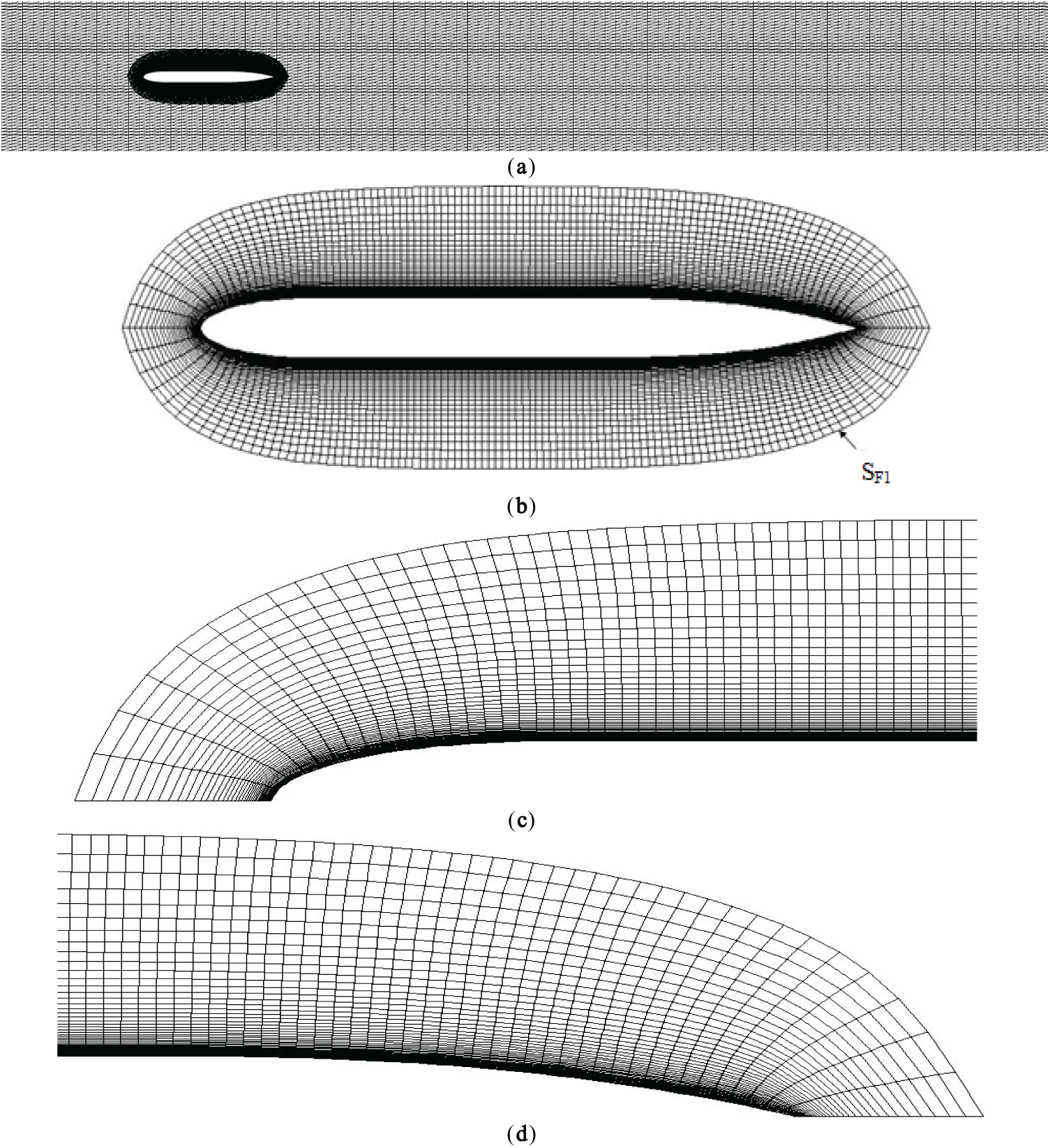
Figure 4: Mesh for Afterbody 1. (a) Mesh in the full domain for Afterbody 1; (b) Mesh in the Ω1 for Afterbody 1; (c) Mesh near the nose; (d) Mesh near the tail

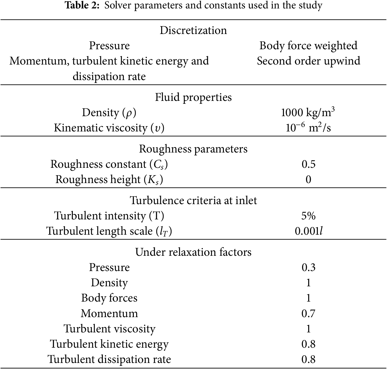
The k-ω SST (shear stress transport) model is used to introduce turbulence into the simulation while solving RANS equations, where ω is the rate of dissipation and k is the turbulent kinetic energy. No-slip boundary condition has been imposed on the surface of the body SB. The velocity inlet boundary condition with velocity as U m/s in the x-direction has been imposed on the boundary AB (refer to Fig. 3). The pressure outlet boundary condition with pressure equal to gauge pressure (p = 0) has been imposed on the boundary CD. The gradients of ω and k are also set to zero on the boundary CD. Zero shear stress condition has been imposed on the remaining four boundaries (two top boundaries, BC, AD and two side boundaries not visible in Fig. 3, being 2D). The solver parameters set during the numerical experimentation in CFD software are reported in Table 2.

The computation of the flow field around a body involves solving the conservation equations of fluid motion, namely the mass, popularly known as the continuity equation and momentum, popularly known as the Navier-Stokes equations. Upon time averaging, these conservation equations lead to well-known RANS equations. The continuity equation in an incompressible flow can be written as:

∂Ui∂xi=0(4)

where Ui is the instantaneous velocity component.

The Navier-Stokes equations of motion can be written in the following form:

ρ∂Ui∂t+ρ∂(UjUi)∂xj=ρRi+∂σij∂xj(5)

where Ri is volume force σij is the total stress, σij for a Newtonian fluid, can be written as:

σij=−Pδij+2μ(Sij)(i,j=1,2)(6)

where P is the pressure (Pa), δij is Kronecker’s delta, and Sij is the strain-rate and is defined as:

Sij=12(∂Ui∂xj+∂Uj∂xi)(i,j=1,2)(7)

The Reynolds-averaged Navier-Stokes equations can be derived from Eqs. (1) and (2) by splitting Ui, in time mean velocity ui, and time fluctuating velocity u″i, making Ui=ui+u″i P, in time mean pressure p, and time fluctuating pressure p″, making P=pi+p″. The time average of the continuity equation and the Navier-Stokes equations is defined as:

∂U―i∂xi=∂ui∂xi=0∂ui∂t+∂(ujui+u″iu″j―)∂t=R―i−1ρ∂p∂xi+∂∂xj(ν(∂uj∂xi+∂ui∂xj))(8)

where ν = μ/ρ is the kinematic viscosity of the fluid (m2/s). −ρu″iu″j― is the Reynolds stress. Eq. (5) is popularly known as the RANS equations, and these equations cannot be solved directly as they no longer remain a closed set and require additional equations. It is through these additional equations that turbulence makes their imprint upon the mean velocity and pressure. The problem now is that the time averaging has created a tensor of unknowns. Since ρu″iu″j― it is symmetric, there are six additional unknowns. This is called the closure problem. The turbulence model aims to express the Reynolds stress in known or calculable quantities. In Cartesian coordinates, the components of the viscous stress tensor which represents an additional momentum transfer due to turbulent fluctuations are defined through Boussinesq approximation for incompressible flows as:

ρu″iu″j―=−μT(∂uj∂xi+∂ui∂xj)+23ρkδij(9)

where μT=νT/ρ is the turbulent viscosity as the constant of proportionality and k is the kinetic energy. As the Reynolds stresses are not known, appropriate turbulence models are introduced for modelling these stresses and their interaction with the mean flow variables. Several turbulence models have been proposed in the past for both high-ReL and low-ReL applications, as the behavior of turbulence is expected to be different in fully turbulent and transitional flows. SST k-ω turbulence model is used in the present study and their applicability and relevance in the context of flow past axisymmetric bodies is critically examined.

4  Optimization Problem and Its Solution by Genetic Algorithm

The design optimization problem considered to be solved in this work consists of a single objective function (i.e., either minimization of drag or minimization of delivered power or minimization of drag-to-lift ratio), subjected to constraints on geometric parameters, total volume and total length. The mathematical formulation of the problem can be as follows:

Minimize F(x1,…,x5) subject to constraints l+x1+x2=cl;g(x1,…,x5)≥cg.

And variable bounds

xLi≤xi≤xUi(i=1,2,…,5)(10a)

Three different optimization problems were treated in this work to optimize the shape of Afterbody 1. The problems stated are as follows:

1.   Problem P1. Minimize drag F(x1, … , x5). This problem, involving five design variables (as discussed in Section 2) and two design constraints, namely, total volume and total length of the vehicle, seeks an optimum shape across all practical ranges of speeds. The mathematical form of the problem can be stated as:

F=D(Drag),x1=Lf,x2=La,x3=nf,x4=nax5=rm,l=Lp,cl=L=3.066 m

g=∇(volume),cg=0.148m3(10b)

and

x1L=0.1 m,x2L=0.5 m,x3L=x4L=1,x5L=0.125 m,(10c)

x1u=x2u=1.5m,x3u=x4u=10,x5u=0.175m.

2.   Problem P2. Minimize drag-to-lift ratio (D/L) F(x1, … , x5). This problem also involves five design variables and two design constraints as discussed above and seeks an optimum shape for the bare hull having an angle of attack (α = 6°). The mathematical representation of the problem is as follows:

F=DL(Drag/lift),x1=Lf,x2=La,x3=nf,x4=nax5=rm,l=Lp

cl=L=3.066 m,g=∇(volume),cg=0.148m3(10d)

and

x1L=0.1 m,x2L=0.5 m,x3L=x4L=1,x5L=0.125 m,(10e)

x1u=x2u=1.5 m,x3u=x4u=10,x5u=0.175 m.

3.   Problem P3. Minimize delivered power (PD) F(x1, …, x5). This problem involves six design parameters, five for the bare hull shape and one for the duct inclination of the ducted propeller. The mathematical representation is given below:

F=PD(Delivered Power),x1=Lf,x2=La,x3=nf,x4=nax5=rm,l=Lp

x6=θ;cl=L=3.066 m,g=∇(volume),cg=0.148m3(10f)

and

x1L=0.1 m,x2L=0.5 m,x3L=x4L=1,x5L=0.125 m,x6L=5∘,

x1u=x2u=1.5 m,x3u=x4u=10,x5u=0.175 m,x6u=15∘.(10g)

The linear constraint has been solved adopting (first of Eq. (10a,d,f) ‘Genetic Algorithm for Numerical Optimization for Constrained Problems (GENOCOP)’ discussed in Miettinen et al. [26], Michalewicz and Attia [27].

5  Numerical Implementation

As mentioned above, the current focus is to create a design framework for the design of axisymmetric shapes where optimization is carried out by heuristic algorithms, namely, genetic algorithms and the objective which is of hydrodynamic nature can be evaluated solving RANS equations with appropriate boundary conditions set and physics of the problem in the simulation. The important task is to seamlessly integrate GA with geometry generator, CFD preprocessor (to generate domain and mesh around the body), CFD solver and CFD post-processor (to obtain the drag values). In other words, we need to embed the geometry creation, mesh generation and CFD solution into an automatic implementation of the GA to ensure that there is no need for manual intervention to set the parameters for the CFD solver to estimate values of the objective functions.

The convergence of the total drag (D) using CFD calculations is reported in Fig. 5 for a single forward speed (U = 15 m/s). Fig. 5 also depicts the convergence of total drag (D) for the optimum shape achieved using the proposed methodology for speed U = 15 m/s. It is clear from Fig. 5 that a minimum of 4000 iterations is needed to claim the convergence of total drag. However, at nearly 2000 iterations, one can notice the periodic oscillating nature with attenuation of the drag force, which implies the possibility of calculating accurately the converged drag force as the mean value of these oscillations (with respect to iterations). To reduce the total time taken by the design framework, it is therefore decided to use 2000 iterations for all intermediate variants during the optimization process instead of going up to 4000 to 6000 iterations for drag convergence. However, the drag of the optimum configuration is obtained by running the CFD solver up to 4000 to 6000 iterations for high accuracy.

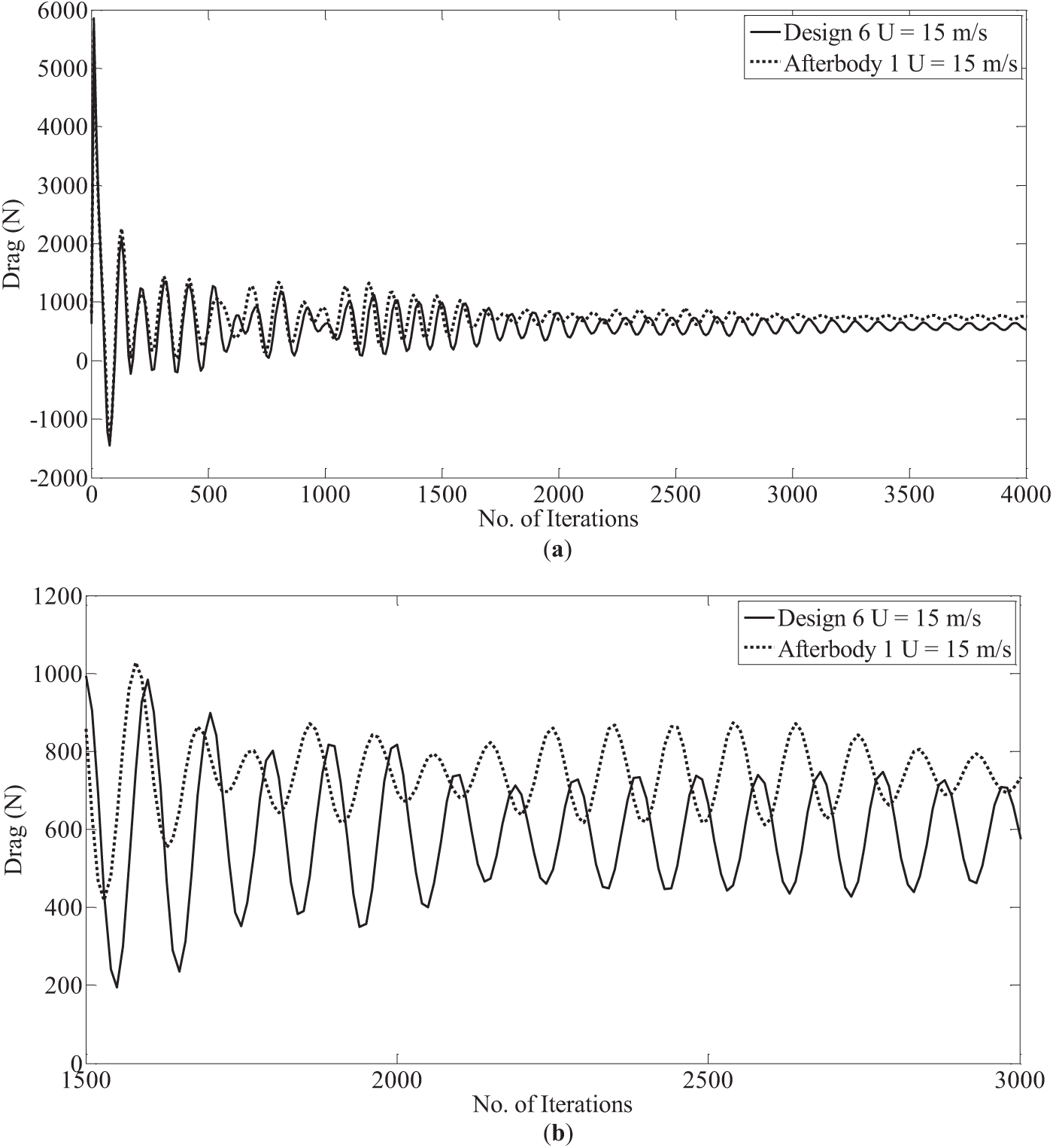
Figure 5: Comparison of convergence of the total drag (D) for Afterbody 1 and Design 6 at U = 15 m/s. (a) Full range of iterations; (b) Partial range of iterations

6  Results and Discussion

6.1 CFD Validation

As mentioned above, Huang et al. [25] conducted experimental studies on A1 in a wind tunnel for a single Reynolds number, namely, Re = 6.6 × 106. The results of these wind tunnel experiments were used by many researchers later to validate their CFD methodology; the exhaustive list is Sarkar et al. [28,29], Virag et al. [30] and Shereena et al. [31]. All of them used different inlet turbulence intensities and turbulence models. Also, they all used water as the surrounding fluid around A1. Table 3 reports the comparison of experimental measurements, a few existing CFD calculations reported in literature and present CFD calculations of hydrodynamic drag for A1. It is evident from the table that the CFD calculations reported in this study are in good agreement with experimental measurements. The good accuracy of the current calculations is further supported by Fig. 6, where the comparison of pressure coefficient (Cp) on the body surface between the present calculations to that of experimental results for the region reported in Huang et al. [25] (i.e., 0.65 ≤ x/L ≤ 1).

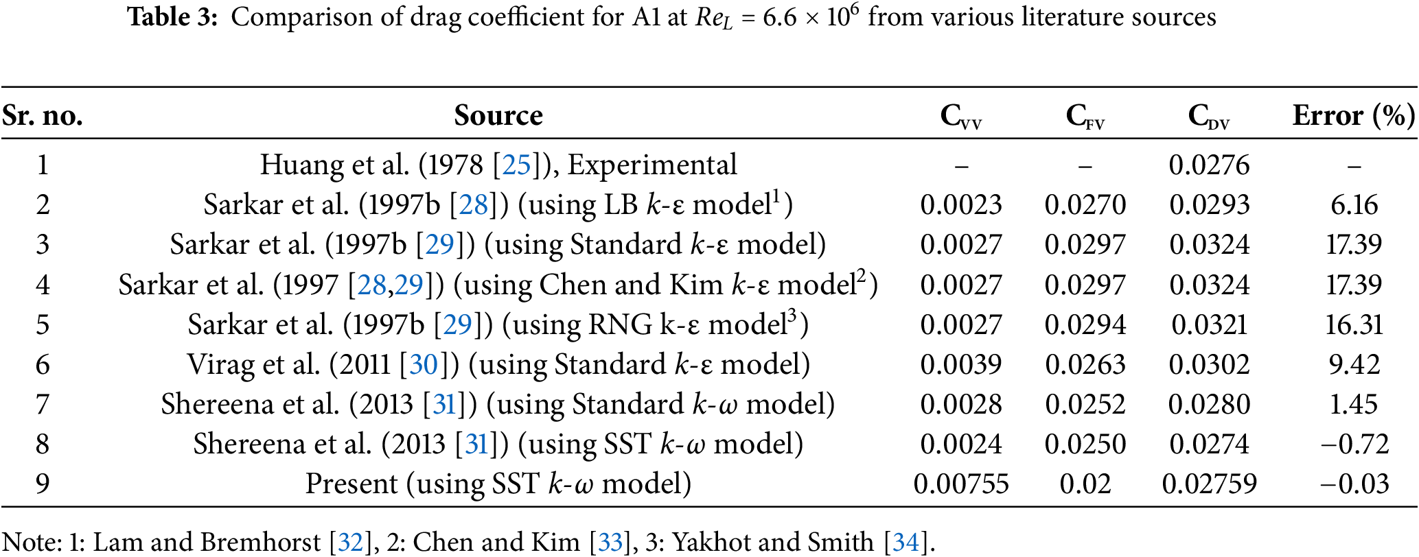
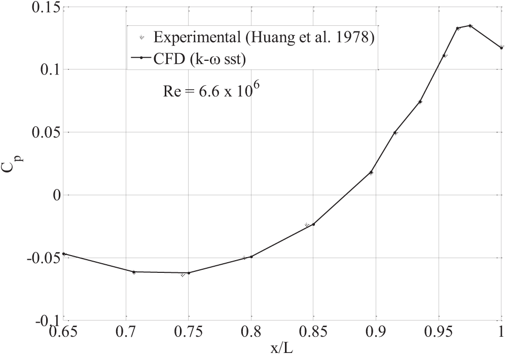
Figure 6: Comparison of computed and measured tail pressure distribution on Afterbody 1 [25]

The grid independence study is not presented in this work because a very fine mesh has been used in the current work than those works reported in Table 3. For example, in this work, there are approximately 1 million cells, whereas the results reported by Shereena et al. (2013) were for 0.25 million cells.

Optimization Results of Problem P1

The optimization of the parent hull A1 is carried out for six forward speeds of the vehicle, namely, U = 0.5 m/s (= U1), 1 m/s (= U2), 1.5 m/s (= U3), 2.152 m/s (= U4), 10 m/s (= U5) and 15 m/s (= U6). The first four speeds are in the typical range of AUVs, and the last two are much above the typical range. We denote the optimized shape for Uj as D j (j = 1 to 6). The convergence of the hull shape parameters (x1 to x5 in Eq. (10)) with successive iteration cycles (i.e., ‘generation’ in GA parlance) is presented in Fig. 7 for three speeds, namely U = 2.152 m/s, 10 m/s, 15 m/s (i.e., U4, U5 and U6). From the figure, it is evident that the optimization process runs till 22 iterations, even though it is sufficiently converging at 13 iterations, considering all speeds. Fig. 8 presents the convergence of total drag force with successive generations for the same three speeds (i.e., U4, U5 and U6). The hull shapes of the parent hull and all six optimized shapes are given in Fig. 9 and Table 1.

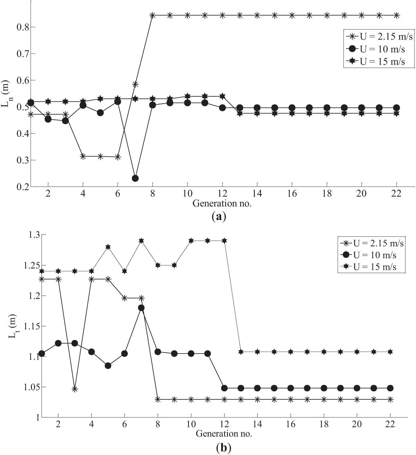
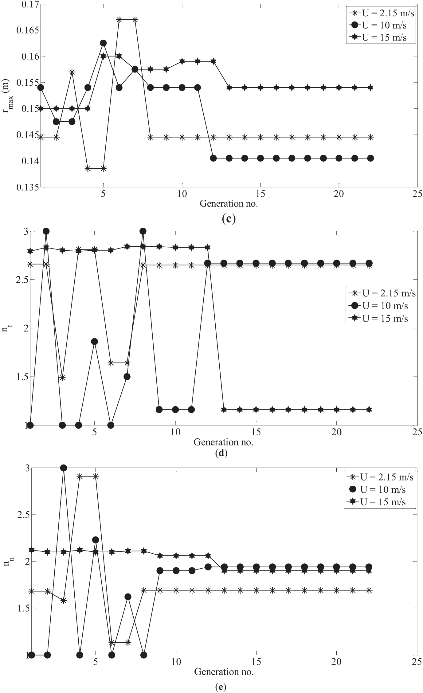
Figure 7: Evolution of the design parameters over successive generations. (a) Variation of nose length; (b) Variation of tail length; (c) Variation of maximum radius; (d) Variation of tail parameter; (e) Variation of nose parameter

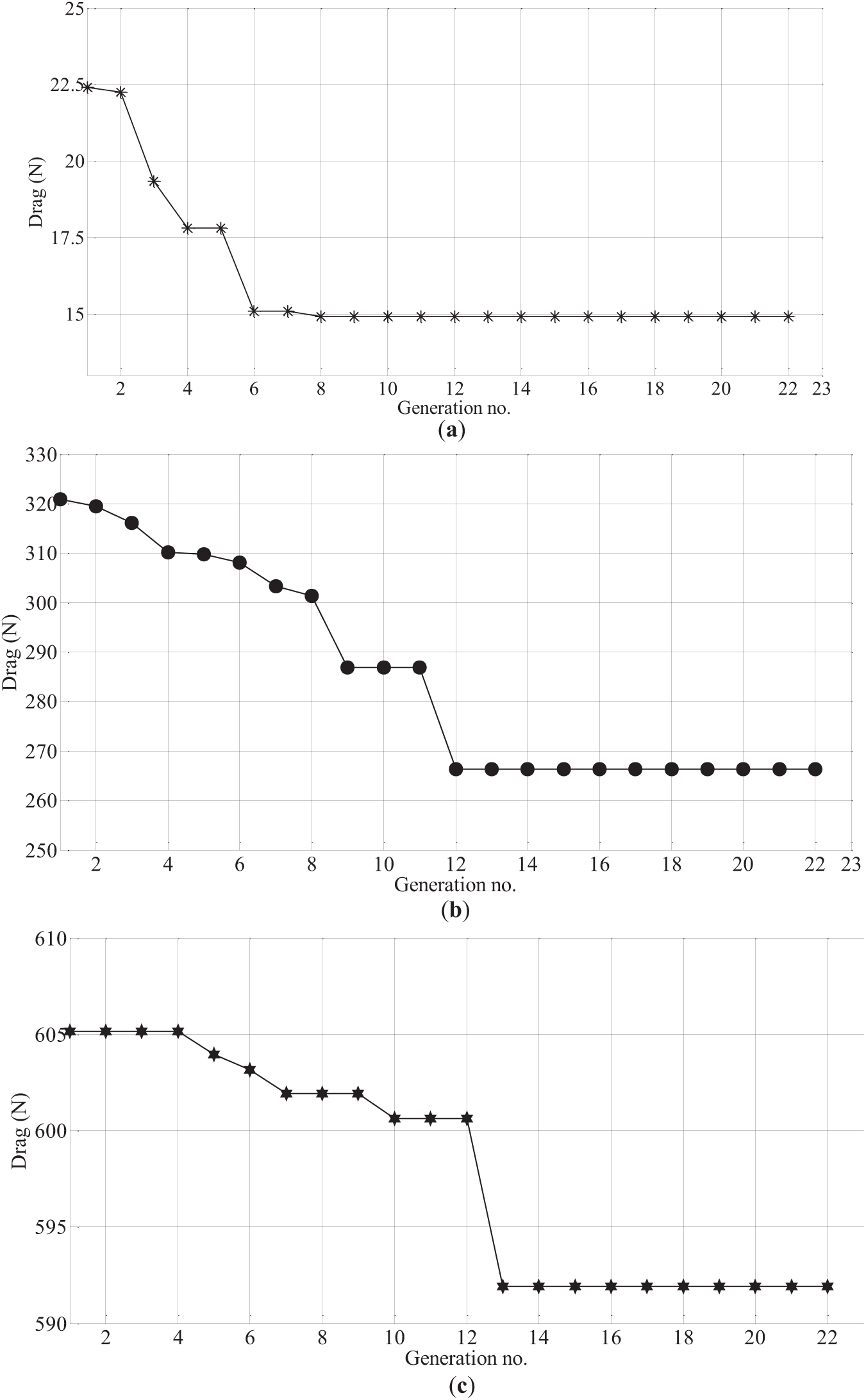
Figure 8: Evolutionary history of the optimization for Design 4, Design 5 and Design 6. (a) Evolution of drag values for optimization with U = 2.152 m/s; (b) Evolution of drag values for optimization with U = 10 m/s; (c) Evolution of drag values for optimization with U = 15 m/s

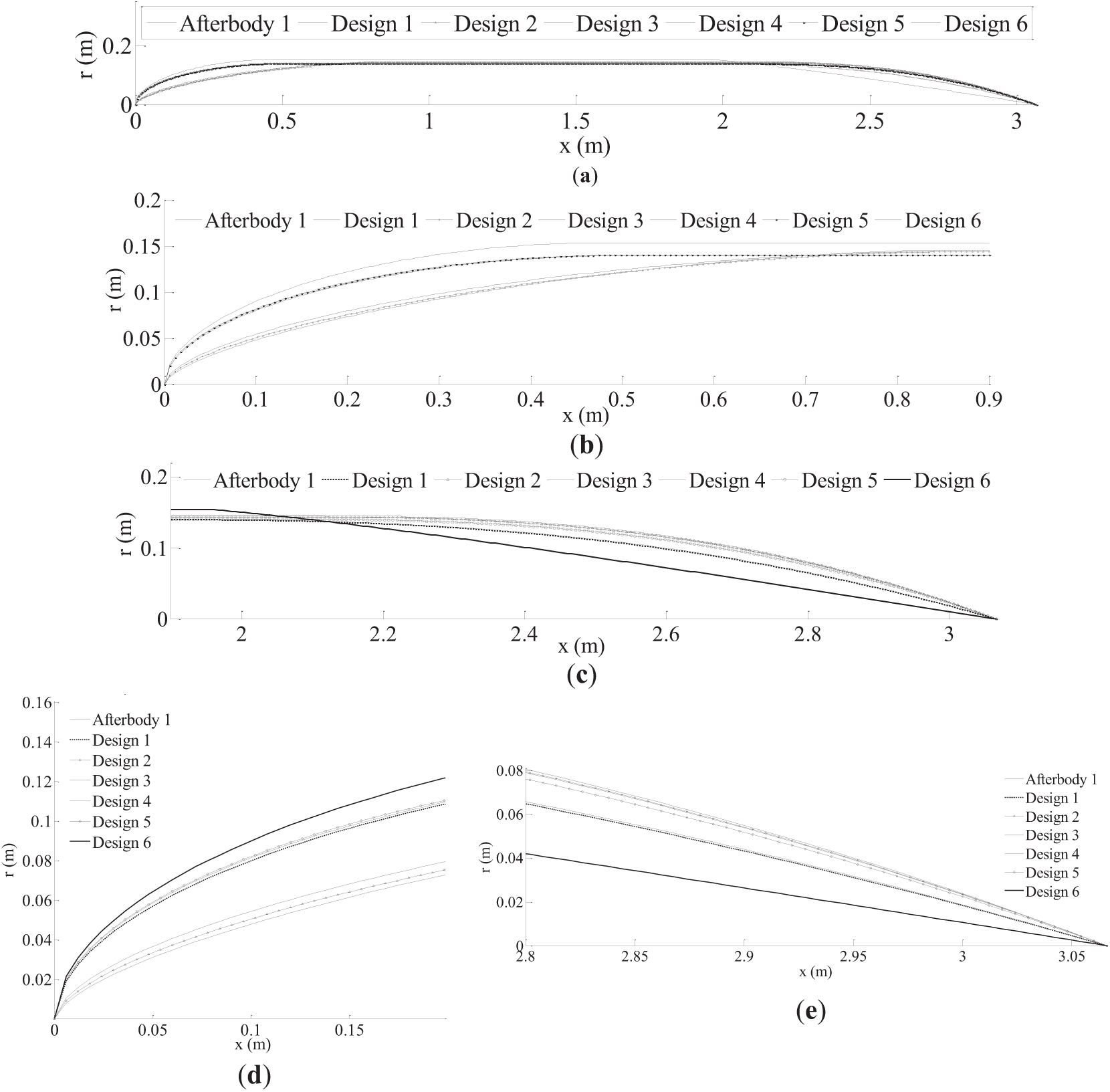
Figure 9: Geometries of Afterbody 1 and Designs 1 to 6. (a) Hull comparison; (b) Nose shape; (c) Tail shape; (d) Close view of nose shape; (e) Close view of tail shape

The drag forces for the parent hull (A1) and six optimized shapes (D1 to D6), with the drag reduction of the optimized shapes concerning the parent hull, are recorded in Table 4. As can be seen that Dj (j = 1 to 6) are the shapes of minimum drag for the speed Uj. The drag reductions are quite substantial, 17.5%, 22.2%, 21.74%, 14.84%, 20.31% and 24.35% for U1 to U6, respectively. It is seen that all six optimized shapes have lower drag than the parent hull for all six forward speeds.

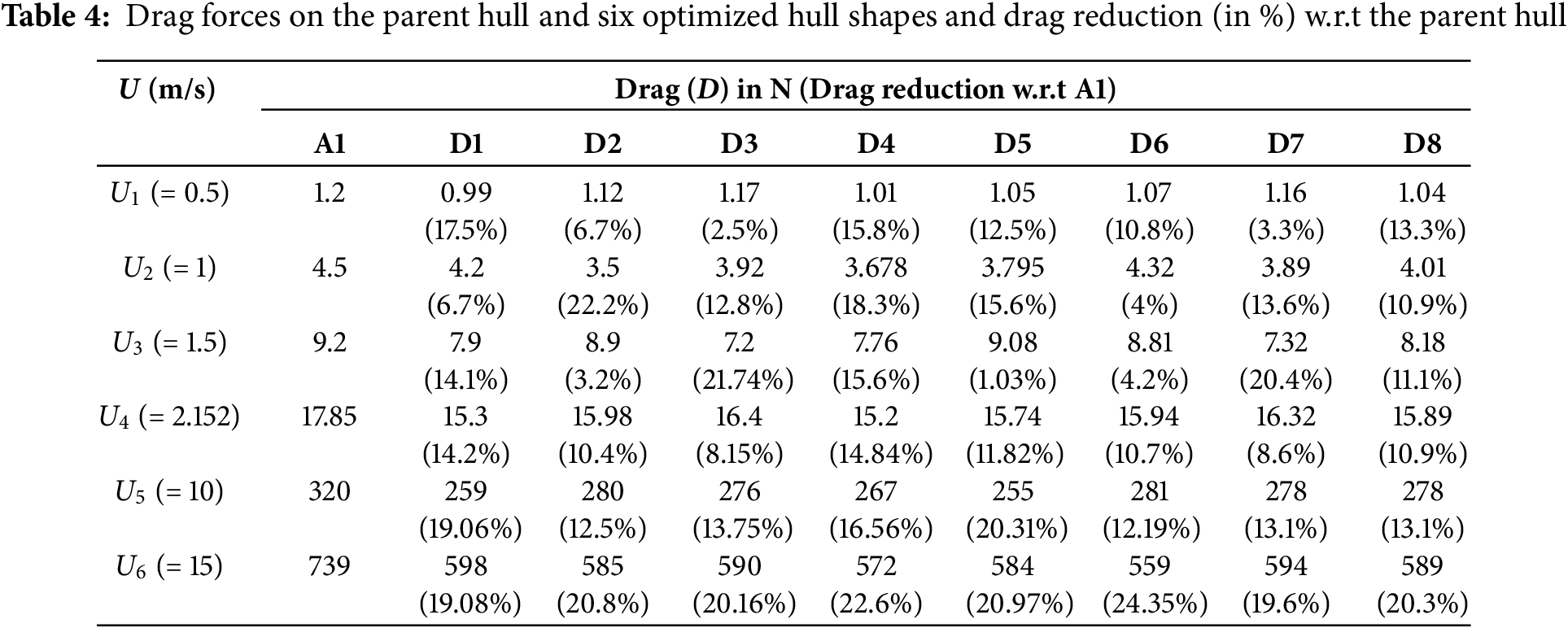
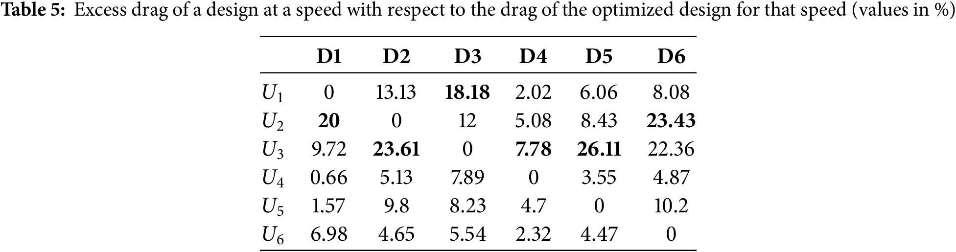
Denoting the drag of Dj at speed Ui by Dij(i, j = 1 to 6), and bearing in mind that Min{Dij(j=1,2,…,6)}=Dii one can construct D¯ij=100(Dij−Dii)/Dii so that D¯ij the excess drag Dj at speed Ui over the drag of the optimized design at this speed (i.e., Dij), expressed in percentage. The values Dij are presented in Table 4 and those of D¯ij are given in Table 5, which shows that maximum values in each column are 20%, 23.16%, 18.18%, 7.78%, 26.11% and 23.43% for D1 to D6, respectively. These values are the largest of the excess drag of Dj considering all six speeds, and are given by Dj′=max{D¯ij(i=1,2,…,6)}. The design with the minimum Dj′, which in this case is D4 (an excess of 7.78%), is the design that will work best for all speeds. It may also be seen that if one considers the typical speed range of AUVs alone, given by Ui (i = 1 to 4), even then, the D4 is the best design in that speedrange.

From Fig. 9, it is observed that the nose shapes of A1, D1 and D5 are close, and the nose shapes of D2, D3 and D4 are close. Also, the tail shapes of A1 and D1 are close, and the tail shapes of D3, D4 and D5 are close. The total drag coefficient (CDV) and the percentage of skin friction drag component (CFV) and viscous pressure drag component (CVV) in CDV for all seven configurations at all six speeds are presented in Table 6. The frictional drag component is dominating over the viscous pressure drag component in the total drag. The percentage variations are in the narrow but high range of 72.66% to 94.8% for all six speeds for the six optimized configurations. Fig. 10 presents the variations of the pressure coefficient of D5, D4 and D6 along the length of the vehicle in comparison with the A1 for U = 2.152, 10 and 15 m/s, respectively.

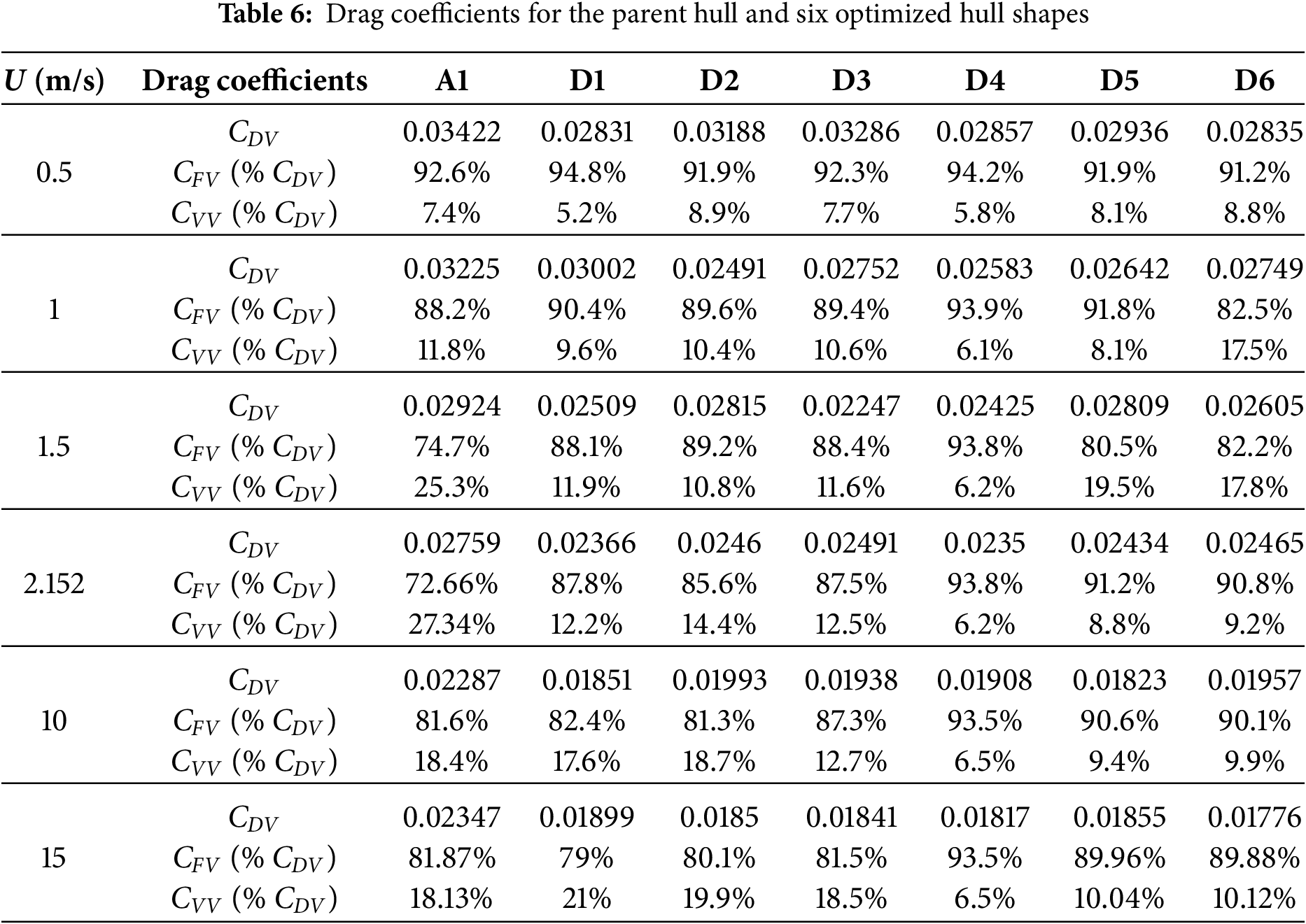
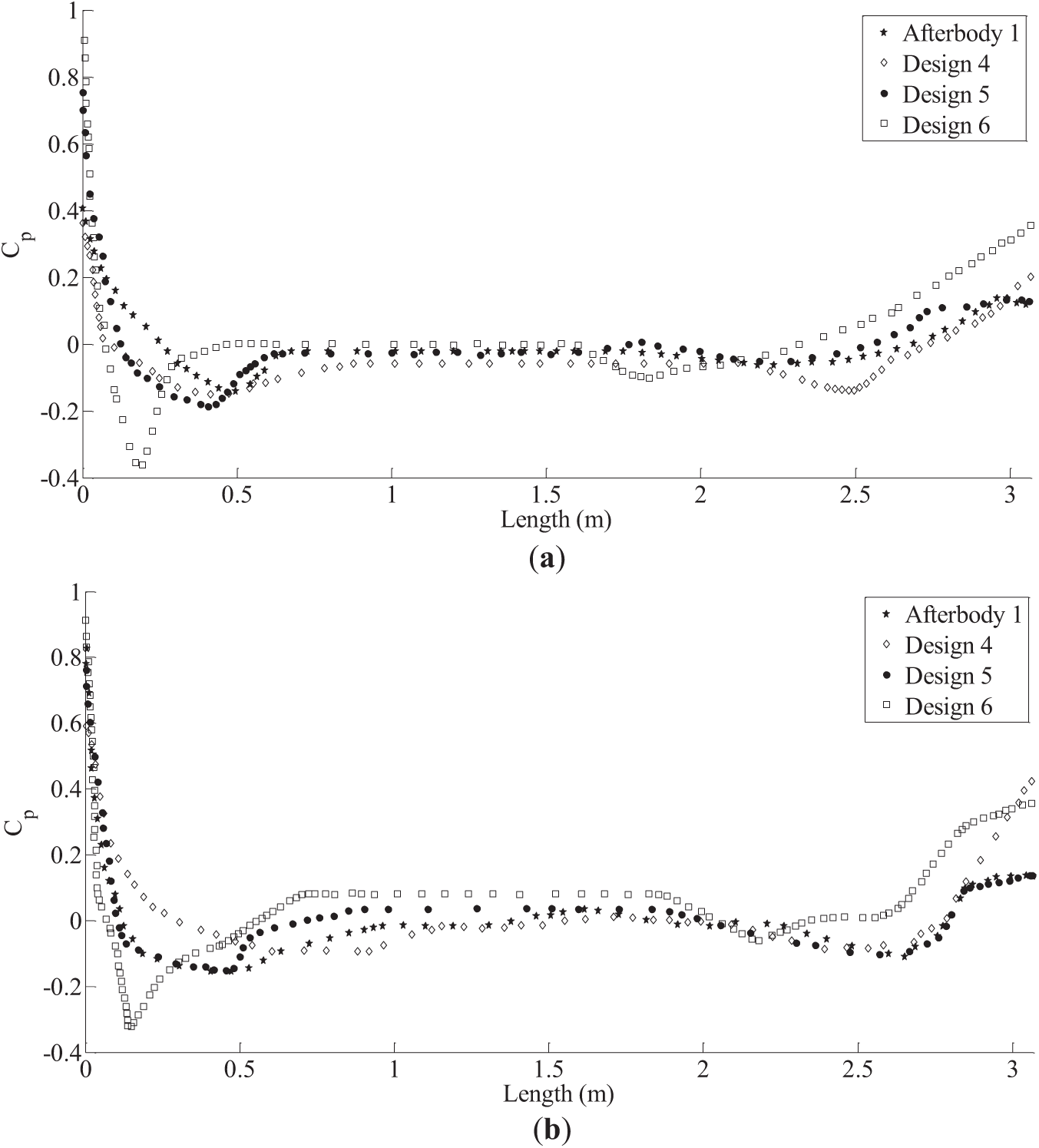
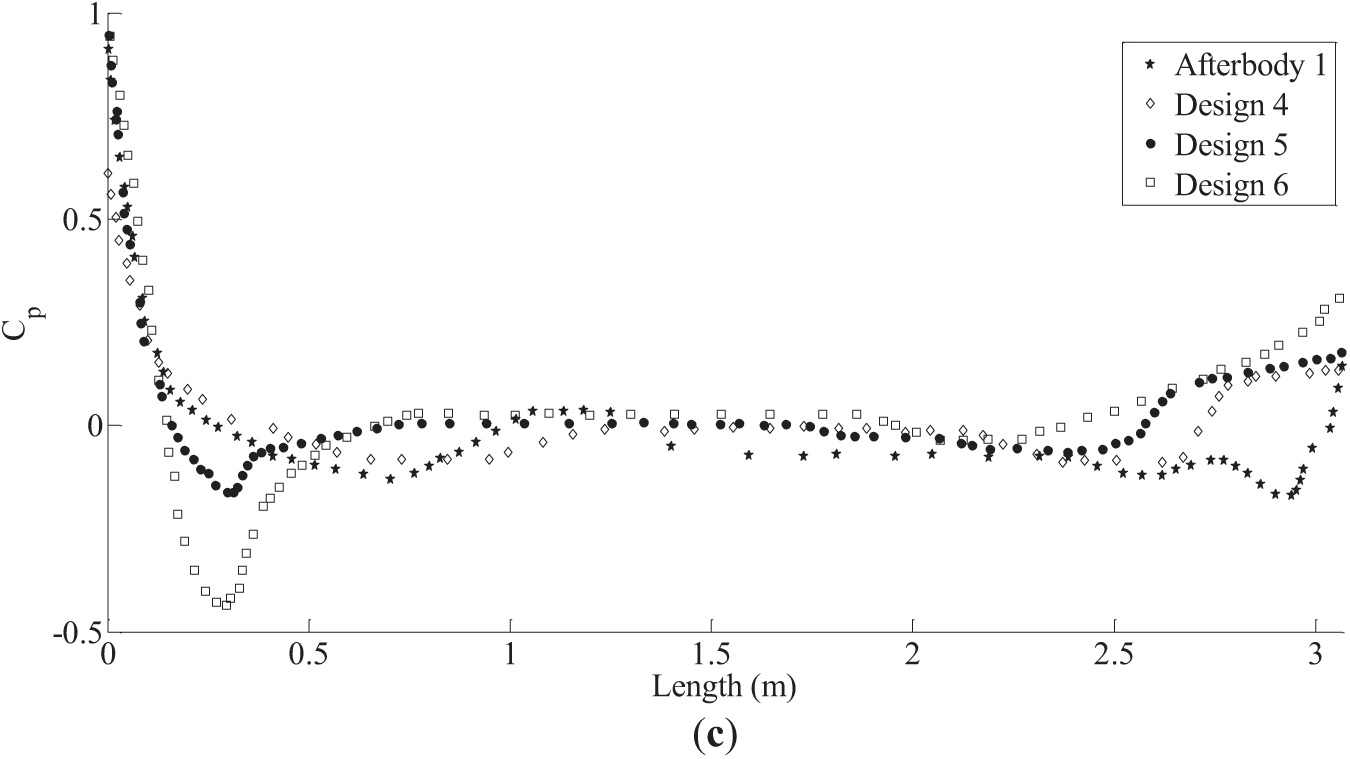
Figure 10: Variations of the pressure coefficients. (a) U = 2.152 m/s; (b) U = 10 m/s; (c) U = 15 m/s

Optimization Results of Problem P2

The D/L minimization of A1 is solved for a single speed, U = 1 m/s and single angle of attack, α = 6° and for a single speed. The resulting shape is denoted D7. The hull shape comparison between A1, D4 (which is the ‘least drag’ considering all speeds at α = 0°) and D7 are presented in Table 1 and Fig. 9. From Fig. 9, it can be seen that D7 has a fuller nose than both A1 and D4. L, D and L/D ratios of the three designs (i.e., A1, D4, D7, D8) for various angles of attack, namely, α = 2°, 4°, 8°, 10° and 12° at U = 1 m/s, are recorded in Table 7. It can be noticed from Table 7 that both D4 and D7 have larger L/D than A1 for all angles of attack.

Further, D7 performs better than D4 at angles of attack upto α = 6°, whereas D4 performs better than D7 at angles of attack in the range 6° < α < 12°. The drag of D4 is less than that of D7 over the full range of α. From this, it may be concluded that D4 will be a better design choice than D7 even when L/D ratio is considered. It should be noted that the L/D will play a significant role for vehicles with wings (e.g., AUG). It will be interesting to study this optimization problem when lifting surfaces are present in the hull, though such a study is not carried out in the present work.

Optimization Results of Problem P3

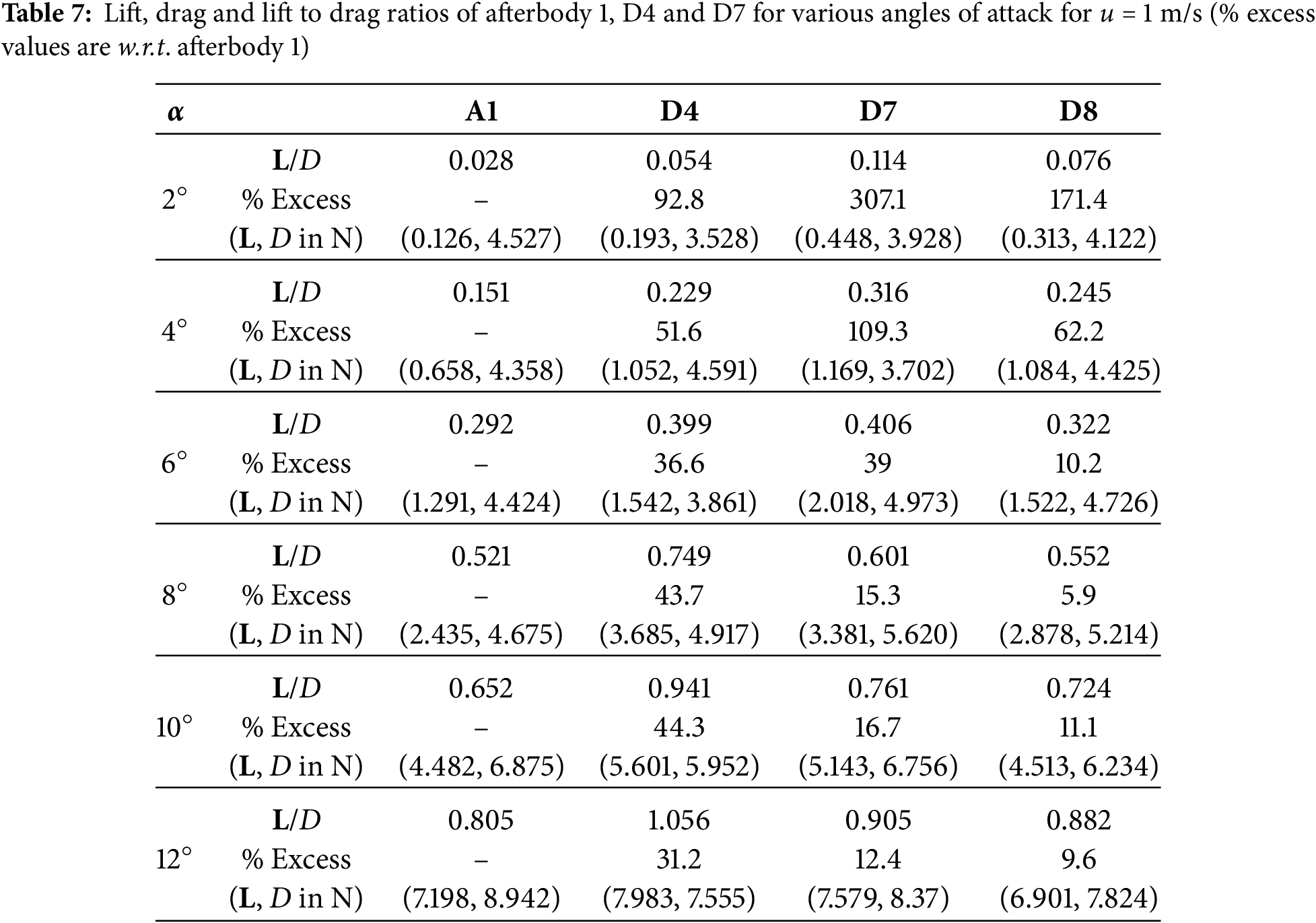
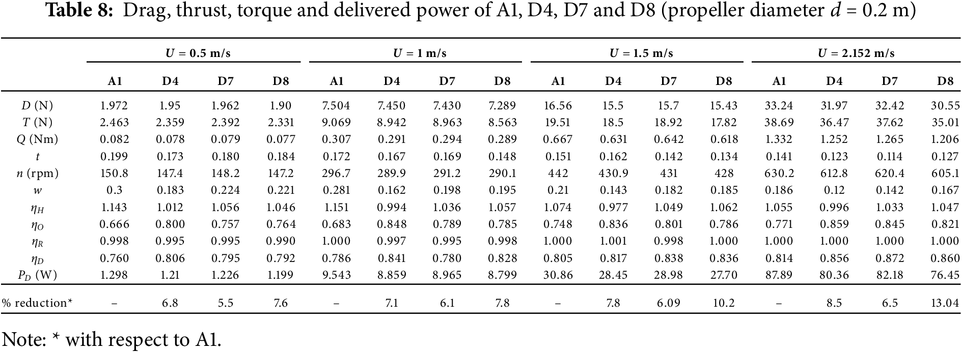
D8 is the shape obtained as a result of solving the delivered power (PD) minimization of A1 for speed (U = 2.152 m/s). The CFD convergence for the coefficient of thrust and coefficient of torque is reported in Fig. 11. The scale for the coefficient of thrust is on the left side of the plot, whereas the scale for the coefficient of torque is reported to the right of the plot for U = 1 m/s. From Fig. 12, it is evident that for convergence, 1500 iterations are sufficient, but we carried out up to 2000 iterations. The comparison of hull shapes D4, A1, D7 and D8 is presented in Table 1 and Fig. 12. It can be noticed that the parallel middle body length (Lm) of D8 is less than D4, A1 and D7; therefore, to satisfy the volume constraint, its diameter is increased by 8%, 11% and 12%, respectively. From the figure, it can be seen that D8 has a finer nose when compared to the other 3 shapes (D4, A1 and D7), whereas its tail has a closer match with D4. Table 7 records the values of thrust (T), Hydrodynamic drag (D), torque (Q), thrust deduction factor (t), propeller rpm (n), efficiencies, delivered power (PD) and effective wake fraction (w) of the four designs (i.e., D4, D7, D8 and A1) for three velocities (U = 1, 1.5 and 2.152 m/s). From Table 7, it can be noticed that D4 (i.e., has the least D) is outperforming other shapes in terms of hydrodynamic drag for U = 1, 1.5 and 2.152 m/s, respectively. The hydrodynamic drag reduction of D8 when compared to D4 is 8%, 5% and 4% for speeds U = 1, 1.5 and 2.152 m/s, respectively. The reduction is not very significant at higher speeds. Table 8 depicts that D8 (least PD) is better in terms of delivered power than D4, A1 and D7. The reduction of delivered power between D8 and D4 is not significant at low speeds, but its significance is increasing with speed; the reductions reported as 0.6%, 2.6% and 4.9% for U = 1, 1.5 and 2.152 m/s, respectively. This underscores the importance of the optimization of delivered power over that of hydrodynamic drag. It may be happening because the interaction between the hull and the propulsion system has been ignored while optimizing for hydrodynamic drag and L/D. This highlights the importance of optimizing the entire system (including appendages, control fins, rudders, and propeller) rather than the bare hull. While considering bare hull alone for optimization, one may end up ignoring the interaction of fluid near the intersection of appendages to the bare hull, and this may lead to a design that is not optimum.

Figure 11: CFD convergence of coefficients of thrust and torque for Afterbody 1 at U = 1 m/s

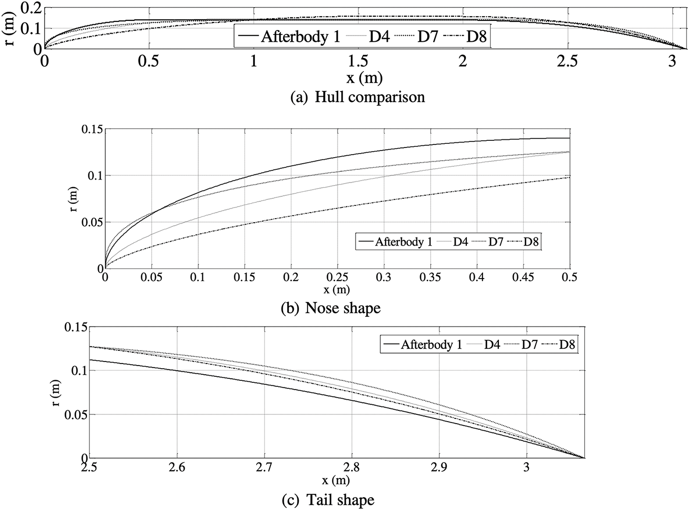
Figure 12: Geometries of Afterbody 1, D4, D7 and D8

It will be interesting to study the above optimization problem with lifting surfaces on the bare hull as in general the major contribution to lift is coming from lifting surfaces than the bare hull itself. The future direction of this work may go in this direction.

7  Conclusion

This work reports the effective use of genetic algorithms as an efficient optimization tool to find solutions for the design problem of AUVs with axisymmetric shape. It also compares the results achieved by solving the drag minimization problem, lift-to-drag maximization problem and delivered power minimization problem in the design of AUVs. The hull of the AUV is described by a 5-parameter formula. No appendages were used in the drag minimization and lift-to-drag maximization problems, but a ducted propeller is attached to the hull when the delivered power minimization problem is solved with only duct angle as the sixth parameter of the optimization process. It seems that the optimum design (D8) achieved by solving maximizing delivered power outperforms both the optimum designs achieved by solving for drag minimization (D4) and L/D maximization (D7), as the objective functions. The results are promising and have practical significance. The reduction in delivered power achieved by D8 in comparison with A1 (Afterbody 1) is 7.6%, 7.8%, 10.2% and 13.04%, respectively, for speeds U = 0.5 m/s, 1 m/s, 1.5 m/s and 2.152 m/s. Whereas D4 and D7 are underperforming when the propeller is attached. While considering bare hull alone for optimization, one may end up ignoring the interaction of fluid near the intersection of appendages to the bare hull, and this may lead to a design that is not optimum. This difference is increasing with an increase in the speed of operation of the AUV. The work highlights the importance of considering appendages to the bare hull in the optimization process, and the proposed methodology is capable of handling appendages too. This proposed approach can also be extended to multi-body interaction problems.

Acknowledgement: Not applicable.

Funding Statement: The authors received no specific funding for this study.

Author Contributions: The authors confirm contribution to the paper as follows: study conception and design: KL Vasudev, Manish Pandey; analysis and interpretation of results: Jaan H. Pu. All authors reviewed the results and approved the final version of the manuscript.

Availability of Data and Materials: All data are available in the manuscript.

Ethics Approval: Not applicable.

Conflicts of Interest: The authors declare no conflicts of interest to report regarding the present study.

References

1. Thomas R. Performance evaluation of the propulsion system of the autonomous underwater vehicle C-SCOUT [master’s thesis]. St John’s, NL, Canada: Memorial University of Newfoundland; 2003. [Google Scholar]

2. Alam K, Ray T, Anavatti SG. A new robust design optimization approach for unmanned underwater vehicle design. J Eng Marit Environ. 2012;226(3):235–49. doi:10.1177/1475090211435450. [Google Scholar] [CrossRef]

3. Vasudev KL, Sharma R, Bhattacharyya SK. Multi-objective shape optimization of submarine hull using genetic algorithm integrated with CFD. Proc IMechE Part M J Eng Marit Environ. 2019;233(1):55–66. doi:10.1177/1475090217714649. [Google Scholar] [CrossRef]

4. Parsons JS, Goodson RE, Goldschmied FR. Shaping of axisymmetric bodies for minimum drag in incompressible flow. J Hydronautics. 1974;8(3):100–7. doi:10.2514/3.48131. [Google Scholar] [CrossRef]

5. Ray T, Gokarn RP, Sha OP. A global optimization model for ship design. Comput Ind. 1995;26:175–92. doi:10.1016/0166-3615(95)00003-M. [Google Scholar] [CrossRef]

6. Alexandrov N, Dennis JE JrJr, Lewis RM, Torczon V. A trust region framework for managing the use of approximation models in optimization. Struct Optim. 1998;15(1):16–23. doi:10.1007/bf01197433. [Google Scholar] [CrossRef]

7. Percival S, Hendrix D, Noblesse F. Hydrodynamic optimization of ship hull forms. Appl Ocean Res. 2001;23(6):337–55. doi:10.1016/s0141-1187(02)00002-0. [Google Scholar] [CrossRef]

8. Campana EF, Peri D, Tahara Y, Stern F. Shape optimization in ship hydrodynamics using computational fluid dynamics. Comput Methods Appl Mech Eng. 2010;196(1–3):634–51. doi:10.1016/j.cma.2006.06.003. [Google Scholar] [CrossRef]

9. Tahara Y, Tohyama S, Katsui T. CFD based multi-objective optimization method for ship design. Int J Numer Methods Fluids. 2006;52(5):499–527. doi:10.1002/fld.1178. [Google Scholar] [CrossRef]

10. Peri D, Campana EF. High fidelity models and multi-objective global optimization algorithms. J Ship Res. 2005;49(3):159–75. doi:10.5957/jsr.2005.49.3.159. [Google Scholar] [CrossRef]

11. Alvarez A, Bertram V, Gualdesi L. Hull hydrodynamic optimization of autonomous underwater vehicles operating at snorkeling depth. Ocean Eng. 2008;36(1):105–12. doi:10.1016/j.oceaneng.2008.08.006. [Google Scholar] [CrossRef]

12. Shahid M, Huang D. Computational fluid dynamics based bulbous bow optimization using a genetic algorithm. J Mar Sci Appl. 2012;11(3):286–94. doi:10.1007/s11804-012-1134-1. [Google Scholar] [CrossRef]

13. Goldberg DE. Genetic algorithms in search, optimization and machine learning. Boston, MA, USA: Addison-Wesley; 1989. [Google Scholar]

14. Deb K, Pratap A, Agarwal S, Meyarivan T. A fast and elitist multi-objective genetic algorithm: NSGA-II. IEEE Trans Evol Comput. 2002;6(2):182–97. doi:10.1109/4235.996017. [Google Scholar] [CrossRef]

15. Huang L, Gao Z, Zhang D. Research on multi-fidelity aerodynamic optimization methods. Chin J Aeronaut. 2013;26(2):279–86. doi:10.1016/j.cja.2013.02.004. [Google Scholar] [CrossRef]

16. Vasudev KL, Sharma R, Bhattacharyya SK. Shape optimization of an AUV with ducted propeller using GA integrated with CFD. Ships Offshore Struct. 2017;13(2):194–207. doi:10.1080/17445302.2017.1351292. [Google Scholar] [CrossRef]

17. Tiwari BK, Sharma R. Design and analysis of a variable buoyancy system for efficient hovering control of underwater vehicles with state feedback controller. J Mar Sci Eng. 2020;8(4):263. doi:10.3390/jmse8040263. [Google Scholar] [CrossRef]

18. Patil PV, Khan MK, Korulla M, Nagarajan V, Sha OP. Design optimization of an AUV for performing depth control maneuver. Ocean Eng. 2022;266(5):112929. doi:10.1016/j.oceaneng.2022.112929. [Google Scholar] [CrossRef]

19. Ahmed F, Xiang X, Jiang C, Xiang G, Yang S. Survey on traditional and AI based estimation techniques for hydrodynamic coefficients of autonomous underwater vehicle. Ocean Eng. 2023;268(2):113300. doi:10.1016/j.oceaneng.2022.113300. [Google Scholar] [CrossRef]

20. Chen X, Yu L, Liu LY, Yang L, Xu S, Wu J. Multi-objective shape optimization of autonomous underwater vehicle by coupling CFD simulation with genetic algorithm. Ocean Eng. 2023;286(2):115722. doi:10.1016/j.oceaneng.2023.115722. [Google Scholar] [CrossRef]

21. Hong L, Wang X, Zhang D-S. CFD-based hydrodynamic performance investigation of autonomous underwater vehicles: a survey. Ocean Eng. 2024;305(5):117911. doi:10.1016/j.oceaneng.2024.117911. [Google Scholar] [CrossRef]

22. Sener MZ, Aksu E. The effects of head form on resistance performance and flow characteristics for a streamlined AUV hull design. Ocean Eng. 2022;257:111630. doi:10.1016/j.oceaneng.2022.111630. [Google Scholar] [CrossRef]

23. Lavimi R, Le Hocine AE, Poncet S, Marcos B, Panneton R. Hull shape optimization of autonomous underwater vehicles using a full turbulent continuous adjoint solver. Ocean Eng. 2024;312:119256. doi:10.1016/j.oceaneng.2024.119256. [Google Scholar] [CrossRef]

24. Liu F, Deng X. Multi-objective optimization of an autonomous underwater vehicle shape based on an improved Kriging model. Ocean Eng. 2024;313(1):119388. doi:10.1016/j.oceaneng.2024.119388. [Google Scholar] [CrossRef]

25. Huang TT, Santelli N, Belt G. Stern boundary layer flow on axisymmetric bodies. In: 12th ONR Symposium on Naval Hydrodynamics; 1978 Jun 26–30; Washington, DC, USA. p. 125–67. [Google Scholar]

26. Miettinen K, Makela MM, Toivanen J. Numerical comparison of some penalty-based constraint handling techniques in genetic algorithms. J Glob Optim. 2003;27:427–46. [Google Scholar]

27. Michalewicz Z, Attia NF. Evolutionary optimization of constrained problems. In: Sebald AV, Fogel LJ, editors. Proceedings of the 3rd Annual Conference on Evolutionary Programming; 1994 Feb 24–26; San Diego, CA, USA. River Edge, NJ, USA: World Scientific Publishing; 1994. p. 98–108. [Google Scholar]

28. Sarkar T, Sayer PG, Fraser SM. A study of autonomous underwater vehicle hull forms using computational fluid dynamics. Int J Numer Methods Fluids. 1997;25:1301–13. doi:10.1002/(SICI)1097-0363(19971215)25:11<1301::AID-FLD612>3.0.CO;2-G. [Google Scholar] [CrossRef]

29. Sarkar T, Sayer PG, Fraser SM. Flow simulation past axisymmetric bodies using four different turbulence models. Appl Math Model. 1997;21(12):783–92. doi:10.1016/s0307-904x(97)00102-9. [Google Scholar] [CrossRef]

30. Virag M, Vengadesan S, Bhattacharyya SK. Translational added mass of axisymmetric underwater vehicles with forward speed using computational fluid dynamics. J Ship Res. 2011;55(3):185–95. doi:10.5957/jsr.2011.55.3.185. [Google Scholar] [CrossRef]

31. Shereena SG, Vengadesan S, Idichandy VG, Bhattacharyya SK. CFD study of drag reduction in axisymmetric underwater vehicles using air jets. Eng Appl Comput Fluid Mech. 2013;7(2):193–209. doi:10.1080/19942060.2013.11015464. [Google Scholar] [CrossRef]

32. Lam CKG, Bremhorst KA. Modified form of k-ε model for predicting wall turbulence. J Fluid Eng. 1981;103:456–60. [Google Scholar]

33. Chen YS, Kim SW. Computation of turbulent flows using extended k-ε turbulence closure model. Washington, DC, USA: NASA; 1987. Report No.: NASA CR-179204. [Google Scholar]

34. Yakhot V, Smith LM. The renormalization group, the ε-expansion and derivation of turbulence models. J Sci Comput. 1992;7(1):35–61. doi:10.1007/bf01060210. [Google Scholar] [CrossRef]