Wave Propagation and Chaotic Behavior in Conservative and Dissipative Sawada–Kotera Models

1  Introduction

The article studies the following 5th-order partial differential equation:

∂u∂t+αu2∂u∂x+β∂u∂x∂2u∂x2+γu∂3u∂x3+∂5u∂x5=0,(1)

first considered by Sawada and Kotera in [1] and then by Caudrey et al. in [2]. Eq. (1) describes long waves in water of relatively shallow depth [3]. A generalized Sawada-Kotera equation:

∂u∂t+αu2∂u∂x+β∂u∂x∂2u∂x2+γu∂3u∂x3+d∂2u∂x2+b∂3u∂x3+e∂4u∂x4+∂5u∂x5=0,(2)

is also considered in the article. The Sawada-Kotera Eqs. (1) and (2) are a generalization of the Kawahara equation:

∂u∂t+u∂u∂x+a∂2u∂x2+b∂3u∂x3+e∂4u∂x4+γ∂5u∂x5=0,(3)

which in turn is one of the generalizations of the well-known Kuramoto-Sivashinsky equation:

∂u∂t+u∂u∂x+a∂2u∂x2+b∂3u∂x3+e∂4u∂x4=0.(4)

Eqs. (1), (3) and (4) are widely used to describe wave processes in active and dissipative media when studying models for weakly nonlinear dispersive waves, for which the dispersion terms of more than the third order are significant. This is necessary when modeling the simplest turbulence processes, studying waves at the boundary of two viscous liquids, describing wave phenomena in plasma in toroidal installations, analyzing the behavior of the flame front, and in other problems (see [4]). Eq. (3) also describes waves in shallow water when surface tension and gravitational effects are comparable. The Eq. (4) also arises under exceptional interaction laws for magnetoacoustic waves in plasma propagating at a critical angle relative to the applied magnetic field [4], for long waves in a liquid under an ice cover [5], for longitudinal deformation waves in thin cylindrical shells [6], etc.

At present, the exact soliton solutions of the traveling wave type for Eqs. (3) and (4) and for some special cases of the nonlinear Sawada-Kotera evolution Eq. (1) are quite well studied. Such solutions are found in the form of a function of one variable after a self-similar change of variables in (1) and the transition to a nonlinear system of ordinary differential equations. The resulting system is conservative and possesses many desirable properties, which make it possible to obtain its exact solutions in many cases. For example, its bi-Hamiltonian structure was studied in [7], and a Darboux transformation was received for this system in [8]. In [9–11], some new exact soliton solutions of Eq. (1) were obtained by the bilinear Hirota method [12]. In [13], a direct method was used to find new conservation laws for Eq. (1) in polynomial form. In [14,15], invariant solutions for the Sawada-Kotera equation are found using Lie symmetry groups. A two-mode Sawada-Kotera equation was considered in [16,17]. Some methods for the numerical and analytical soliton solutions of the nonlinear Sawada-Kotera Eq. (1) have been proposed in [18,19]. New soliton wave solutions of a (2 + 1)-dimensional Sawada-Kotera equation were found in [20–22].

The Sawada-Kotera Eq. (1), primarily studied in the context of nonlinear wave theory, exhibits characteristics that can relate to certain phenomena in materials science, particularly in systems involving liquids, such as in complex systems like liquid crystals or ferrofluids [23–25]. Traveling waves and solitons are often observed in materials that exhibit complex rheological properties, such as non-Newtonian fluids, where the fluid’s response to external forces can lead to wave-like phenomena. Moreover, the dissipative nature of the generalized Sawada-Kotera Eq. (2), which can lead to chaotic wave behavior, shares conceptual parallels with chaotic dynamics seen in fluid systems [26–28]. Though the generalized Sawada-Kotera equation does not directly model turbulence, which is a character for the fluid systems in materials science, the principles of bifurcation and chaos that it describes are consistent with the types of behavior seen in many dissipative fluid systems. The principles of nonlinear wave propagation and chaos described by the Sawada-Kotera equations could be applied to better understand fluid dynamics in systems where the behavior is influenced by factors like viscosity, magnetic fields, or particle interactions.

In the present work, a new bifurcation approach developed by the author in [29–31] for all nonlinear systems of differential equations is proposed for the analytical and numerical solution of both the conservative and dissipative Sawada-Kotera equations. This approach makes it possible to find wave solutions that are more complex than soliton ones. In the case of a conservative equation, the method makes it possible to find wave solutions not only in the form of cycles of an ordinary differential equation after a self-similar change of variables but also in the form of two-dimensional and three-dimensional tori, as well as chaotic traveling waves. In the case of a dissipative equation, the method makes it possible to find cascades of bifurcations of stable traveling waves that generate spatiotemporal chaos in the generalized dissipative Sawada-Kotera equation. The technique was applied by the author in [32,33] to find stable and chaotic traveling waves for the Kuramoto-Sivashinsky Eq. (4) and the Kawahara Eq. (3). In article [32], it was proven that for specific parameter values, the Kuramoto-Sivashinsky Eq. (4), in full accordance with the universal bifurcation chaos theory of Feigenbaum-Sharkovsky-Magnitskii (FShM) [29–31], has an endless number of stable wave solutions traveling along the spatial axis with arbitrary speeds, as well as an infinite number of different modes of space-time chaos. The bifurcation parameter is the speed of the traveling wave propagation along the spatial axis. This parameter is not included in the original system of equations. In [33], the analogy result was obtained for the generalized dissipative Kawahara Eq. (3).

2  Conservative Sawada-Kotera Equation

The Sawada-Kotora Eqs. (1) and (2) have significant differences related to the fact that the self-similar change of variables reduces the first equation to a conservative nonlinear system of the fourth order ordinary differential equations, but it reduces the second equation to a dissipative nonlinear system of the fourth-order ordinary differential equation. In this regard, the methods for studying chaotic dynamics in the equations obtained after the self-similar change of variables differ significantly.

2.1 Reduction to an ODE System

Let us consider Eq. (1) on the infinite axis: u(x,t):R×R→R. We will analyze solutions of Eq. (1) using a self-similar replacement of independent variables ξ=x−ct, thereby reducing the original Eq. (1) to a nonlinear ordinary differential equation:

−cu′+αu2u′+βu′u′′+γuu′′′+u′′′′′=0,(5)

where the derivative is taken with respect to ξ. Integrating Eq. (5), we obtain the equation:

−cu+αu33+(β−γ)(u′)22+γuu′′+u′′′′=δ,(6)

where δ is an arbitrary constant. Eq. (6) can be reduced to a nonlinear system of four ordinary differential equations

u˙=v,v˙=w,w˙=z,z˙=cu−αu33−(β−γ)v22−γuw+δ.(7)

If (u(ξ),v(ξ),w(ξ),z(ξ)) is a solution to the ODE system (7), then u(x,t)=u(x−ct) will be a wave solution of the partial derivative system (1).

2.2 Analytical Study of the ODE System

Let us first find the region of dissipativity of the system (7):

divF(u,v,w,z)=∂F1∂u+∂F2∂v+∂F3∂w+∂F4∂z=0,

where the vector function F(u,v,w,z) is the right-hand side of the system of Eq. (7), consequently, the system of Eq. (7) is everywhere a conservative system. This means that system (7) does not have attractors but has a more complex structure of unstable periodic and non-periodic solutions. In this case, traveling waves in Eq. (1) are described by limit cycles, two-dimensional or three-dimensional tori of the system (7), some of them can be born by bifurcations of cycles and tori in an extended dissipative system when its bifurcation parameter tends to zero. So, a conservative system (7) can also have chaotic dynamics as a result of bifurcation cascades in an extended dissipative system (see [29,34]).

Let’s define the singular points (u∗,v∗,w∗,z∗) of the system (7) by equating the right-hand sides of its equations to zero. We get that v∗=0,w∗=0,z∗=0,u∗(c−αu∗2/3)+δ=0. Consequently, the ODE system (7) has three singular points, Oi(u∗i,0,0,0),i=1,2,3, where u∗i are the roots of the cubic equation u∗3−3u∗c/α−3δ/α=0=u∗3+pu∗+q, roots of which are found using Cardano’s formula:

u∗1=a+b,u∗2,3=−a+b2±ia−b23,a=−q2+(p3)3+(q2)23,b=−q2−(p3)3+(q2)23.

When δ=0, then q=0, and O1(u∗1,0,0,0)=(0,0,0,0),O2,3(u∗2,3,0,0,0)=(±3cα,0,0,0).

Let’s define the type and investigate the stability of singular points of the system (7). The linearization matrix of the right side of the system has the form:

A=(010000100001c−αu2−γw−(β−γ)v−γu0),

and its characteristic equation is the equation:

det(A−λI)=λ4+γuλ2+(β−γ)vλ−(c−αu2−γw)=0,(8)

which takes the form λ4+γu∗iλ2−(c−αu∗i2)=0 at the points Oi(u∗i,0,0,0). From the Routh-Hurwitz stability criterion, it follows that all singular points Oi,i=1,2,3, are unstable for all values of the system parameters.

The value δ is the first integral of the system of Eq. (7) and determines the connectedness of variables in the four-dimensional phase space. Therefore, it is natural to expect that for δ>0 the number of different solutions of system (7) and their form will differ significantly from the case with δ=0. In this case, the value δ plays a role inverse to the value of the energy surface level in the analysis of the dynamics of Hamiltonian and conservative systems with connected variables by the constancy of the Hamiltonian or another connection imposed on the variables of the equation. Let us apply the bifurcation approach developed by the author in [34] to the analysis of the dynamics of solutions of the conservative system of Eq. (7).

2.3 Bifurcation Approach to Analysis of Conservative Systems

Modern classical mechanics deals exclusively with a special case of conservative systems: Hamiltonian systems. The theory of Hamiltonian systems reduces the problem of analyzing the dynamics of such systems to the problem of their integrability, i.e., to the problem of constructing a canonical transformation that reduces the system to action-angle variables in which, as is commonly believed, the motion occurs on the surface of a n-dimensional torus and is periodic or quasiperiodic. Any non-integrable nonlinear Hamiltonian system is considered a perturbation of an integrable system, and the analysis of its dynamics is reduced to clarifying the question of the destruction or non-destruction of the tori of the unperturbed system depending on the magnitude of the applied perturbation. The formulation of the last problem is usually called following A. Poincaré [35], the main problem of classical Hamiltonian mechanics, in the solution of which, as is commonly believed, the following significant results have been achieved over the last hundred years [36–40]:

–   It is established by the Kolmogorov-Arnold-Moser (KAM) theory that under certain conditions, most of the non-resonant tori of the unperturbed system are not destroyed by sufficiently small perturbations and continue to exist in the perturbed system;

–   In the case of systems with two degrees of freedom, global stability is preserved since the stochastic layers around the destroyed two-dimensional tori remain squeezed in narrow gaps between the undestroyed invariant tori;

–   In the case of systems with three or more degrees of freedom, even in the case of small perturbations, trajectories can move along the entire accessible energy surface, forming a complex, chaotic structure called the Arnold web;

–   The destruction of resonant tori of the unperturbed system leads to the appearance of so-called islands in the perturbed system—a sequence of hyperbolic singular points (trajectories) connected by separatrices (separatrix surfaces), inside which elliptic singular points (trajectories) are located;

In accordance with the statements above, chaos in a perturbed Hamiltonian system is explained by the effect of the separatrix splitting, when the invariant manifolds of a singular hyperbolic trajectory of the perturbed system begin to intersect, forming a complex tangled chaotic network called a homoclinic or heteroclinic interweaving.

The author proposed in [34] a completely different, bifurcation approach to the analysis of the dynamics of not only Hamiltonian but also any conservative systems of nonlinear differential equations with a given integral. This approach consists of constructing a two-parameter extended approximating dissipative system, the attractors of which are approximations to the solutions of the original Hamiltonian (conservative) system. Such attractors (stable cycles, tori, and singular attractors) of the extended dissipative system can be found by numerical methods in accordance with the results of the universal bifurcation FShM theory [29–31], originally developed for nonlinear dissipative systems of differential equations. The final stage of applying the bifurcation approach is the mandatory final verification of the existence of a close solution (elliptic cycle, torus) in the original Hamiltonian or conservative system.

In the works [29–31], the bifurcation approach is applied to the analysis of several typical perturbed Hamiltonian systems with one and a half, two, two and a half and three degrees of freedom, as well as simply conservative systems, including some classical systems. The results obtained allowed the author to assert that most of the above-listed provisions of classical Hamiltonian mechanics are not satisfied for the considered typical Hamiltonian systems and that the tori existing in these systems are not tori of unperturbed systems for any magnitude of perturbation. The transition to chaos in any such system occurs not through the destruction of some tori of the unperturbed system. It occurs, on the contrary, through cascades of saddle-node bifurcations leading to the effect of multiplication of cycles and tori in the vicinities of the separatrices of the system, and through cascades of bifurcations of the birth of regular and singular attractors in the extended dissipative system as the dissipation parameter tends to zero in accordance with the universal theory of FShM. Thus, the bifurcation approach suggests considering the dynamics of not only Hamiltonian systems, but also any conservative systems as a limiting case of the dynamics of dissipative systems. Within the framework of such a bifurcation concept: a) two-dimensional and multidimensional tori of a perturbed Hamiltonian (and any conservative) system are tori around its main elliptic cycles, formed by the stability regions of close stable cycles of the corresponding extended dissipative system as the dissipation parameter tends to zero and, therefore, have a completely different nature and differ from the tori of unperturbed systems of classical Hamiltonian mechanics, which are by definition Cartesian products of several cycles, and not tori around cycles; b) the complication of the dynamics with an increase in the magnitude of the perturbation in any Hamiltonian (conservative) system begins to occur not as a result of the splitting of the separatrix, but as a result of the non-local effect of the multiplication of cycles and tori in the vicinity of the tangency of various systems of tori along the separatrix surfaces of hyperbolic trajectories (cycles), while the birth of more complex tori occurs around more complex elliptic cycles of the system, close to the stable cycles of the corresponding extended dissipative system, born as a result of saddle-node bifurcations when the dissipation parameter tends to zero; c) the stability regions of complex cycles of a dissipative extended system are not required to generate exclusively tori of the perturbed Hamiltonian (conservative) system around its complex cycles, therefore motion in a perturbed Hamiltonian (conservative) system can occur not only along windings of two-dimensional tori, but also along Möbius bands and other more complex two-dimensional infinitely folded heteroclinic separatrix manifolds characteristic of nonlinear dissipative systems with small dissipation; d) for sufficiently large values of the perturbation magnitude, the transition to chaos in Hamiltonian and conservative systems occurs not through the destruction of some tori of the unperturbed system, but in accordance with the universal theory of FShM through cascades of bifurcations of the birth of tori around elliptic cycles, limiting to stable cycles of extended dissipative systems as the dissipation parameter tends to zero. Let us show that the numerical bifurcation approach is applicable to the analysis of the dynamics of the conservative system of Eq. (7) for different perturbation parameters δ, while the analytical approach of KAM theory is not suitable for solving this problem.

2.4 Numerical Analysis

Let us consider two essentially different cases of the conservative system of Eq. (7): δ=0 and δ=2. For δ=2, the system of Eq. (7) has several elliptic cycles and two-dimensional tori around these cycles, which can be found by solving the system of Eq. (7) under different initial conditions. Fig. 1 shows the projections onto the (v,w) plane of the main two-dimensional torus of the system (7) under u0=1.9 and its section by the z=0 plane, as well as different sections of the energy surface of the system of Eq. (7) by the z=0 plane under δ=2 and the initial conditions: (1.6<u0<4.5;v0=0,w0=0,z0=0.1).

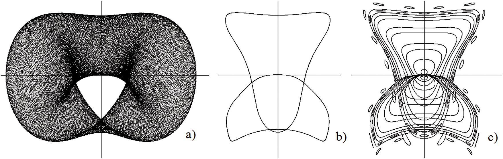
Figure 1: (a–c) Projections onto the (v,w) plane of the main two-dimensional torus of the system (7) under u0=1.9 and its section by the z=0 plane, as well as different sections of the energy surface of the system of Eq. (7) by the z=0 plane under δ=2 and the different initial conditions: (u0=1.65;1.75;1.86;1.9;2.1;2.4;2.6;3;3.2;3.5;4;v0=0,w0=0,z0=0.1)

Fig. 2 presents the projections onto the plane (v,w) of an elliptic cycle of the second order existing in the system (7) for δ=2,u0=1.676, a two-dimensional torus around this cycle for u0=1.65 and its section by the plane z=0.

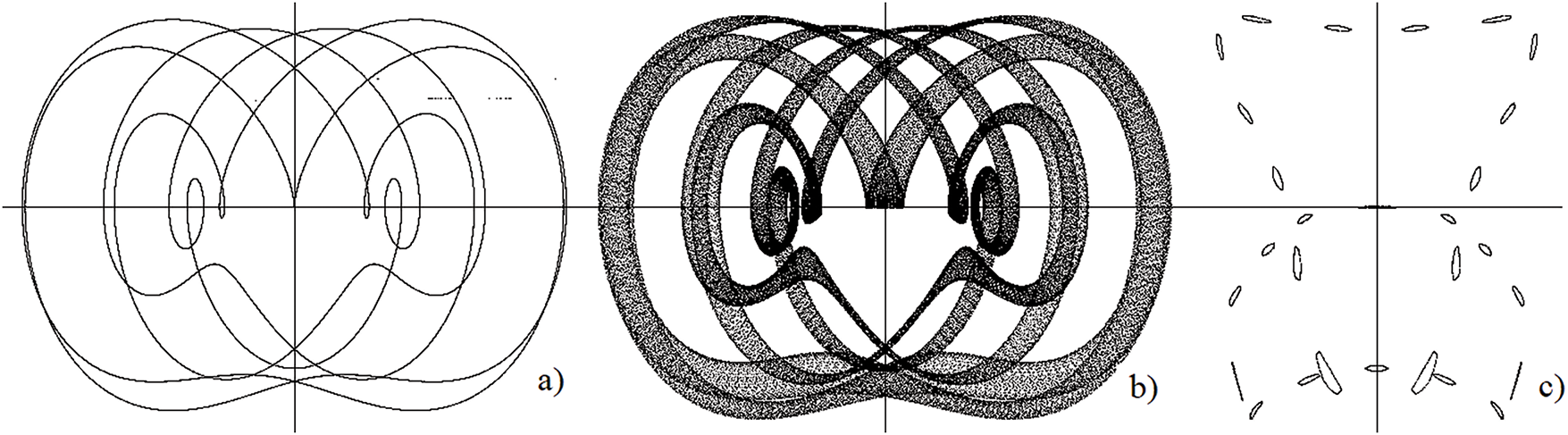
Figure 2: (a–c) Projections onto the (v,w) plane of an elliptic cycle of the second order of the system (7) at δ=2,u0=1.676, a two-dimensional torus around this cycle for u0=1.65 and its section by the plane z=0

Analysis of the dynamics of solutions of the system of Eq. (7) for δ=2 shows that, in this case, the system has its solutions either simple basic elliptic limit cycles or two-dimensional tori around such cycles tangent along hyperbolic cycles. In full accordance with the bifurcation approach, around the basic elliptic cycle of the first order and the two-dimensional torus around it (Fig. 1a,b) in the system, there are elliptic cycles of the second order (Fig. 2a) and more complex tori around them (Figs. 1c and 2b,2c). All cycles of the system can be found as a result of solving the extended dissipative system when the dissipation parameter tends to zero.

When δ=0 the situation becomes noticeably more complicated. In this case, in addition to the main elliptic cycles and two-dimensional tori around them, as well as elliptic cycles and two-dimensional tori of the second order (Fig. 3), the system of Eq. (7) has elliptic multi-turn cycles and two-dimensional tori of the third order (Fig. 4a,b).

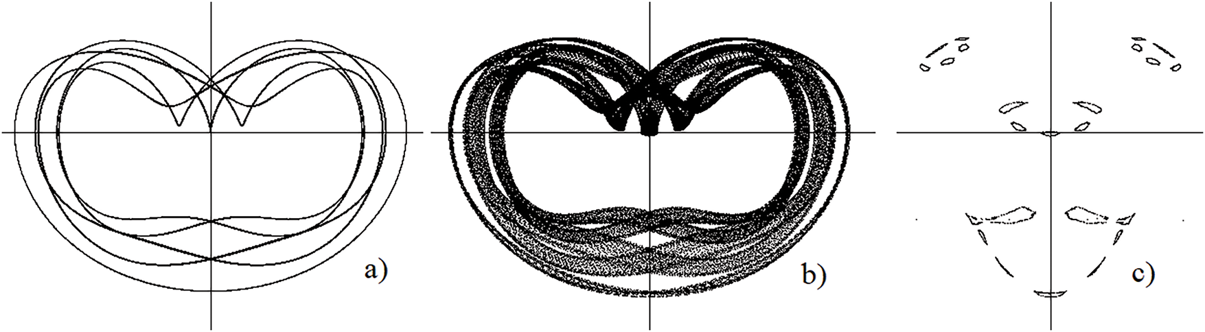
Figure 3: (a–c) Projections onto the (v,w) plane of an elliptic cycle of the second order of the system (7) at δ=0,u0=1.67, a two-dimensional torus around this cycle for u0=1.62 and its section by the plane z=0

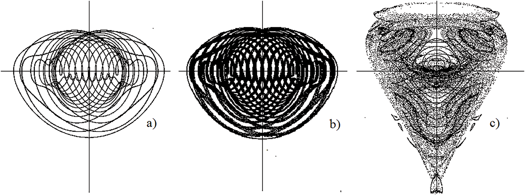
Figure 4: (a–c) Projections onto the (v,w) plane of an elliptic cycle of the third order of the system (7) at δ=0,u0=4.325, a two-dimensional torus around this cycle for u0=4.2986 and its section by the plane z=0, as well as different sections of the energy surface of the system of Eq. (7) by the z=0 plane under δ=0 and the different initial conditions: (u0=0.21;08;1.2;1.5;1.62;1.8;2.1;2.3;2.7;3;3.8;4.2;4.35;4.4;4.45;4.5,v0=0,w0=0,z0=0.1)

As follows from the bifurcation approach to the analysis of conservative systems, multi-turn third-order tori arise as a result of the effect of the multiplication of cycles and tori in the neighborhoods of separatrix manifolds. As a result, either a transition to chaotic dynamics occurs in their neighborhoods, or three-dimensional tori are born. Both cases look like chaos in the first Poincaré section z=0, which is clearly demonstrated in Fig. 4c. Therefore, in order to give an unambiguous answer to the question of what is actually depicted in Fig. 4c, chaos or a three-dimensional torus, it is necessary to take the next section of codimension 2 in the three-dimensional space generated by the section z=0 of codimension 1, for example, u=const. Taking the second section on the solution of the system of Eq. (7) with the initial condition u0=4.45, we obtain a closed curve in it (Fig. 5c), which indicates that the chaos in the first section, depicted in Fig. 5b, is in fact a three-dimensional torus.

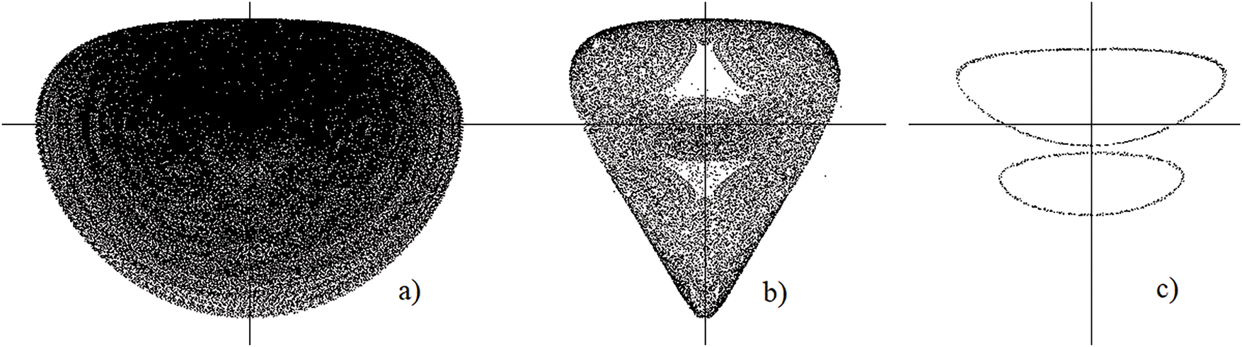
Figure 5: Projections onto the (v,w) plane of the three-dimensional torus of the system (7) at δ=0,u0=4.45 (a); its section of codimension 1 by the plane z=0 (b); and two sections of codimension 2 by the planes u=const (c)

Thus, the topology of the conservative system (7) for large values of the parameter δ is determined by the main two-dimensional tori around the main cycles of the system. For smaller values of the parameter δ, the topology of the system (7) is determined not only by the two-dimensional tori around the main cycles of the system but also by the three-dimensional tori around the two-dimensional tori. For the considered values of the parameter δ, it was not possible to detect regions with chaotic dynamics, although it is quite possible that such regions may exist. The appearance of chaos is created by points lying in the Poincaré sections on the surfaces of complex tori formed by the stability regions of the complex cycles of the extended dissipative system of equations as the dissipation parameter tends to zero. Next, we consider the dissipative generalized Sawada-Kotera Eq. (2), which, as will be shown below, already has chaotic dynamics.

3  Generalized Sawada-Kotera Equation

The main difference between generalized Sawada-Kotera Eqs. (2) and (1) is the presence of a positive coefficient at the fourth derivative with respect to the spatial variable, which leads to the dissipativity of the equation and, consequently, the possibility of the existence of its solutions in the form of arbitrarily complex stable periodic and chaotic waves running along the spatial axis with different speeds. Unlike the conservative Sawada-Kotera Eq. (1), the analysis of the dynamics of solutions of the dissipative Eq. (2) can be carried out directly using the results of the universal bifurcation chaos theory of Feigenbaum-Sharkovsky-Magnitskii.

3.1 Reduction to an ODE System

We will also consider the Eq. (2) on the entire number line: u(x,t):R×R→R. We will analyze regular and chaotic solutions of Eq. (2) using a self-similar replacement of independent variables ξ=x−ct, thereby reducing the original Eq. (2) to a nonlinear ordinary differential equation:

−cu′+αu2u′+βu′u′′+γuu′′′+du′′+bu′′′+eu′′′′+u′′′′′=0,(9)

where the derivative is taken with respect to ξ. Integrating Eq. (9), we obtain the equation:

−cu+αu33+(β−γ)(u′)22+γuu′′+du′+bu′′+eu′′′+u′′′′=δ,(10)

where δ is an arbitrary constant. Eq. (10) can be reduced to a nonlinear system of four ordinary differential equations:

u˙=v,v˙=w,w˙=z,z˙=cu−αu33−(β−γ)v22−γuw−dv−bw−ez+δ.(11)

If (u(ξ),v(ξ),w(ξ),z(ξ)) is a solution to the ODE system (11), then u(x,t)=u(x−ct) will be a wave solution of the partial derivative system (2).

3.2 Analytical Study of the ODE System

Let us first find the region of dissipativity of the system (11):

divF(u,v,w,z)=∂F1∂u+∂F2∂v+∂F3∂w+∂F4∂z=−e,

where the vector function F(u,v,w,z) is the right-hand side of the system of Eq. (11), consequently, the system of Eqs. (11) is everywhere dissipative system when e>0. In this case, traveling waves in Eq. (2) are described by limit cycles or tori of the system (11), traveling impulses are described by loops of separatrices of saddle-focuses of the system (11), and chaotic dynamics in Eq. (2) is described by singular attractors of the system (11) in the sense of the bifurcation FShM chaos theory.

Let us consider the case δ=0 and find the singular points (u∗,v∗,w∗,z∗) of the system (11) by equating the right-hand sides of its equations to zero. We get that: v∗=0,w∗=0,z∗=0,u∗(c−αu∗2/3)=0. Consequently, the ODE system (11) has three singular points: O(0,0,0,0),O±(±3c/α,0,0,0). Let us study the stability and type of singular points of the system (11). The linearization matrix of the right-hand side of the system has the form:

A=(010000100001c−αu2−γw−(β−γ)v−d−γu−b−e),

and its characteristic equation is the equation:

det(A−λI)=λ4+γuλ2+(β−γ)vλ−(c−αu2−γw)=0,

which takes the form λ4−c=0 at the point O(0,0,0,0), and

λ4+eλ3+(±γ3c/α+b)λ2+dλ+2c=0,(12)

at the points O+ and O−. From the Routh-Hurwitz stability criterion, it follows that the singular point O is unstable for all values of the system parameters, and the stability conditions for the singular points O+ and O− have a kind of

e(γu∗+b)>d,e(γu∗+b)d−2e2c>d2.(13)

Let us consider the singular point O+(3c/α,0,0,0). Let the value c∗ be the leading root of the equation e(γ3c/α+b)d−2e2c−d2=0 for fixed positive values of the parameters e,b,d,γ,α. Then, obviously, for c<c∗ both conditions (13) of stability of the singular point O+ are satisfied. For c>c∗, the singular point O+ loses stability.

Theorem 1: For any fixed positive values of the parameters e,b,d,γ,α, the singular point O+(3c/α,0,0,0) is a stable focus for c<c∗. For c>c∗ the singular point O+ loses stability, and a stable limit cycle is born from it as a result of the Andronov-Hopf bifurcation.

Proof: Let c∗ be such a value of the parameter c for which the characteristic Eq. (12) at the singular point O+ has two purely imaginary complex conjugate roots λ3,4=±iω. Then having written the characteristic polynomial (12) in the form:

λ4+eλ3+(γ3cα+b)λ2+dλ+2c=(λ−λ1)(λ−λ2)(λ2+ω2)=0,

and equating the coefficients at the same powers of λ, we get that

{λ1+λ2=−e,λ1λ2+ω2=(γ3c∗/α+b),(λ1+λ2)ω2=−d,λ1λ2ω2=2c∗.(14)

Solving the system of Eq. (14), we find that in this case λ1+λ2=−e,ω2=d/e,λ1λ2=2ec∗/d, and, therefore, 2ec∗/d+d/e=(γ3c∗/α+b) and

λ1,2=−e2±e24−2ec∗d,c∗=dγ4e3α+3d2γ216e2α−(d2−bde)2e2.

The obtained equation for the value of c∗ coincides with the stability condition (13) of the singular point O+ obtained from the Routh-Hurwitz criterion, up to a positive factor de. Therefore, for c<c∗ the singular point O+ is stable, and, in addition, two eigenvalues λ1,2 of the linearization matrix of system (11) at this singular point are negative real numbers, and the other two eigenvalues λ3,4 are complex conjugate numbers with a negative real part. Consequently, for c<c∗ the singular point O+ of system (11) is a stable focus, and for c>c∗ the singular point O+ loses stability with the birth of a stable limit cycle from it as a result of the Andronov-Hopf bifurcation. The theorem is proved. □

It follows from the theorem that the greatest interest is in the study of possible cascades of bifurcations of stable singular point O+ in the case where its first bifurcation is Andronov-Hopf bifurcation of the birth of stable limit cycle, that is, for c>c∗. In this case, all three cascades of bifurcations of stable limit cycles and an infinite number of chaotic singular attractors can exist in the system of Eq. (11) in accordance with the bifurcation FShM chaos theory. And in this case, the generalized Sawada-Kotera Eq. (2) can have an infinite number of complex periodic and non-periodic (chaotic) traveling waves, up to traveling impulses.

Analytical study of bifurcations of the Eq. (11) and the generalized Sawada-Kotera equation following the Andronov-Hopf bifurcation with increasing values of the parameter c for singular point O+ starting with the period-doubling bifurcations of the born limit cycles, is an extremely difficult task. For this purpose one must analytically find the multipliers of the cycle, that is almost not possible, and determine such values of the parameter c for which one of the multipliers is equal to +1, the second is equal to −1, and the other two multipliers lie inside the unit circle of the plane of the complex variables. Therefore, we will further study the complexity of the dynamics of solutions to the generalized Sawada-Kotera equation using numerical methods.

3.3 Scenario of Transition to Dynamical Chaos

Let us carry out a numerical study of the system (11) for fixed values of the parameters e=1,δ=0,d=1,b=1,γ=1,α=1,β=5. For these parameter values, we find that c∗=3/2 or c∗=3/4. Numerical calculations confirm that for c∗<0.75 the singular point O+(3c∗,0,0,0) is a stable focus, and for c∗>0.75 a stable limit cycle is born from it. This cycle remains stable up to the value c∗≈1.17. At c∗≈1.17, stable limit cycle C2 of the double period is born from it. When the values of the parameter c are further increasing, the Feigenbaum period-doubling cascade of bifurcations is observed. Period 4 cycle is born at c≈1.253, period 8 cycle is born at c≈1.2714 etc. At c≈1.277 in Eq. (11), there is the simplest singular (chaotic) attractor-the Feigenbaum attractors-non-periodic trajectory that is the limit of cycles from the Feigenbaum cascade of period-doubling bifurcations (Fig. 6).

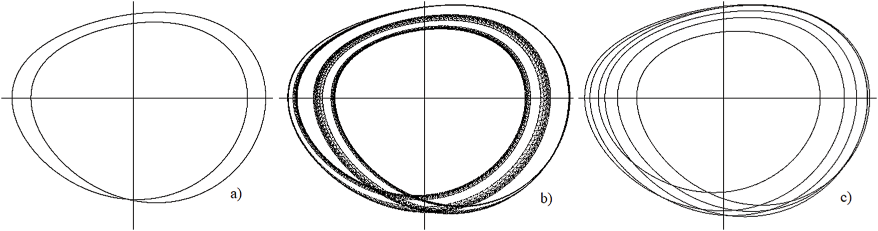
Figure 6: Projections on the plane (v,w) of the cycle C2:(a) of period 2, the Feigenbaum attractor (b) and the cycle C6:(c) of period 6 of the subharmonic cascade of bifurcations of the system of Eq. (11), found at c=1.2,c=1.277 and c=1.284, consequently

With a further increase in the values of the parameter c, the stable cycles are born in accordance with the Sharkovsky order, and then they are born in accordance with the homoclinic order. So, for example, stable cycle C6 of period 6 of the subharmonic Sharkovsky cascade of bifurcations is detected at c=1.284 (Fig. 6), and a stable cycle C5 of period 5 is detected at c=1.303 (Fig. 7). A stable cycle H4 of the homoclinic cascade of bifurcations, making 4 conventional turns in a spiral around the saddle-focus O+, is detected at c=1.3558 (Fig. 7b). As is known (see [29–31]), the sequence of cycles of a complete homoclinic cascade must converge to a saddle-focus separatrix loop. It is quite possible that the separatrix loop exists for a given set of values of the system parameters, because one of the complex singular (chaotic) attractors, found in the system of Eq. (11) at c=1.355, has quite a small eye (Fig. 7c). The detection of the separatrix loop in the space of seven parameters of the system e,δ,d,b,γ,α,β is a very difficult task, since the manifold on which the loop exists has codimension two or even three or more.

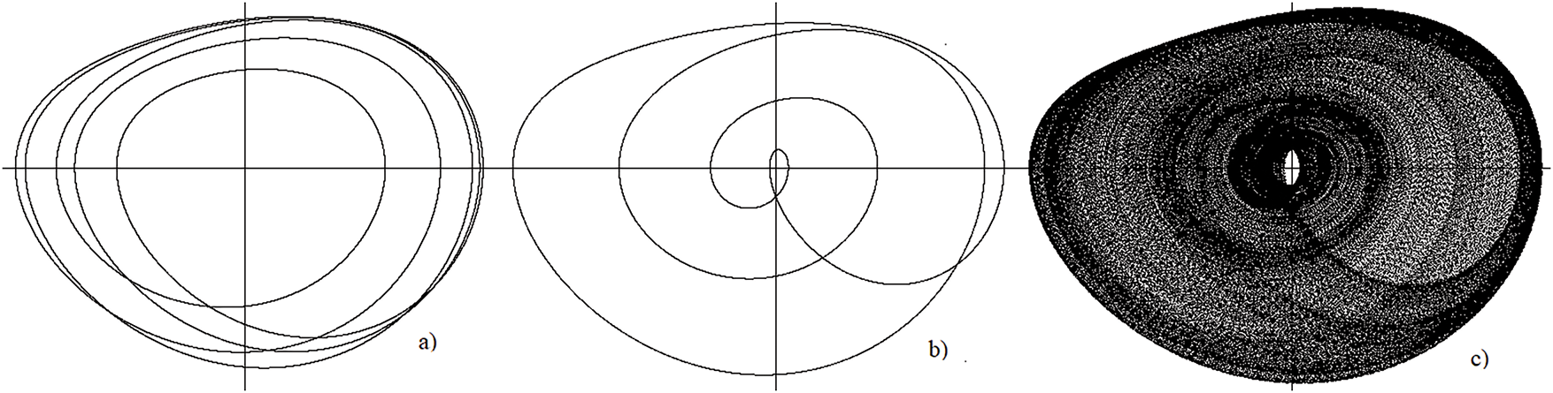
Figure 7: Projections on the plane (v, w) of the cycle C5:(a) of period 5 of the subharmonic cascade of bifurcations, cycle H4:(b) of period 4 of the homoclinic cascade of bifurcations, and one of the complex singular attractors (c), found in the system of Eq. (11) at c=1.303,c=1.3558 and c=1.355, consequently

Fig. 6 shows projections onto the (v,w) plane of stable cycles C2,C6 of periods 2, 6, and Feigenbaum attractor of the subharmonic cascade of bifurcations around the singular point O+ when c=1.2,c=1.284 and c=1277.

Fig. 7 shows projections of stable cycle C5 of period 5 of the subharmonic cascade of bifurcations, of stable cycle H4 of period 4 of the homoclinic cascade of bifurcations around the singular point O+, found at c=1.303,c=1.3558, and a complex singular attractor lying in the neighborhood of the separatrix loop of the saddle-focus O+ of system (11) at c=1.355.

Thus, it has been established numerically that in the system (11), when the parameter c changes, there exists a Feigenbaum cascade of period-doubling bifurcations of stable limit cycles, a complete subharmonic cascade of bifurcations of stable cycles in accordance with the Sharkovsky order, and an incomplete homoclinic cascade of bifurcations in accordance with the Magnitskii order. The found cycles and chaotic attractors of the ODE system (11) correspond to the running and chaotic waves of the original generalized Sawada-Kotera Eq. (2). These waves, corresponding to the cycle of period two of the subharmonic cascade, the cycle of period four of the homoclinic cascade, and the singular attractor depicted in Figs. 6 and 7, are presented in Fig. 8.

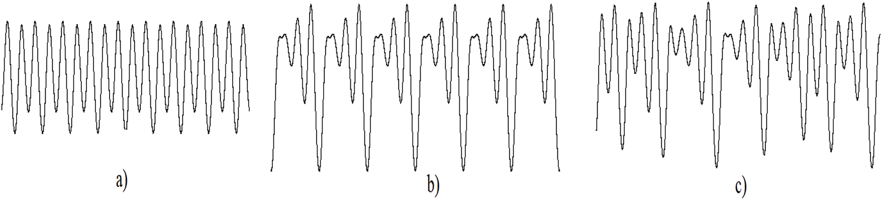
Figure 8: Periodic and chaotic waves u(x,t)=u(x−ct) of the generalized Sawada-Kotera Eq. (2) corresponding to the cycles C2:(a), H4:(b) and chaotic singular attractor (c) of the system (11), depicted in Figs. 6 and 7

Corollary 1: The parameter с is a bifurcation parameter of the system of ordinary differential Eq. (11), but does not explicitly enter into the original generalized Sawada-Kotera Eq. (2). This means that in the original Eq. (2) there are infinitely many different stable and chaotic waves running along the space axis with different speeds.□

Corollary 2: The leading characteristic Lyapunov exponent of any singular attractor of the system (11) is equal to zero.

Proof: The leading characteristic Lyapunov exponent cannot be less than zero since, on any bounded trajectory that does not end at a singular point, one of the Lyapunov exponents in the direction tangent to the trajectory is zero. Let some Lyapunov exponent be greater than zero on a singular attractor, corresponding to some value μ of the bifurcation parameter. For a sequence of smaller values of the bifurcation parameter converging to μ, the system has a sequence of stable cycles of a cascade of period-doubling bifurcations converging to the singular attractor. On each cycle from this sequence, the leading characteristic Lyapunov exponent is zero. Therefore, the limit of this sequence of zero leading characteristic Lyapunov exponents, which is the leading characteristic Lyapunov exponent of the singular attractor, is also zero.□

We presented here a simple proof of the equality to zero of the leading characteristic Lyapunov exponent on any singular attractor without going on to consider complex heteroclinic separatrix manifolds. But as it was rigorously proven in many works of the author and his employees, the FShM theory is the universal bifurcation theory, and there are no other chaotic attractors in this theory except singular ones, i.e., non-periodic bounded trajectories that are the limits of period-doubling bifurcation cascades of some limit cycles. It has also been rigorously proven that any singular attractor lies on a heteroclinic separatrix manifold consisting of exponentially compressed Möbius bands, and so the leading characteristic Lyapunov exponent on any singular attractor is zero.

At the same time, articles continue to be published in the scientific literature on nonlinear and chaotic dynamics, in which the authors, not understanding the essence of the ongoing processes, write about attractors with supposedly found numerically “positive” Lyapunov exponents. It is this fact that is interpreted as the presence of chaotic dynamics in the system. In all such systems with supposedly “positive” Lyapunov exponents without exception, which were studied by the author, the main cycles of the universal bifurcation FShM scenario were found. Systems with other scenarios of transition to chaos were not found. Therefore, all such chaotic systems have indeed only singular chaotic attractors and have no positive Lyapunov exponents. So, the positiveness of the Lyapunov exponent cannot be used as a criterion of chaotic dynamics in a system. The effect of the positiveness of the Lyapunov exponent is exclusively a consequence of computational errors since, due to the presence of an everywhere dense set of non-periodic trajectories, numerical motion is possible only over the entire region in which the trajectory of the singular attractor is located, and not along its trajectory itself. In addition, the calculated numerical Lyapunov exponent will also be “positive” when moving along a stable periodic trajectory of a large period located in the neighborhood of some singular attractor. Therefore, the criterion of chaotic dynamics in any nonlinear dissipative system of differential equations can only be the detection of some reference stable cycles or tori of a cascade of bifurcations in accordance with the Sharkosky-Magnitskii order (cycles or tori of two, six, five or three periods).

4  Discussion

The results obtained in the work demonstrate a wide spectrum of possible complex wave solutions that can have both conservative and dissipative systems of nonlinear partial differential equations. Conservative systems can have only unstable wave solutions, corresponding to solutions of nonlinear conservative systems of ordinary differential equations under self-similar change of variables. Solutions of the latter systems can be elliptic cycles, two-dimensional tori around elliptic cycles, three-dimensional and multidimensional tori generated by two-dimensional tori as a result of the nonlocal effect of multiplication of cycles and tori in the neighborhoods of separatrix surfaces, or as a result of cascades of period-doubling bifurcations of cycles or tori, as well as cascades of more complex bifurcations leading to dynamical chaos in ODE systems or to spatio-temporal chaos in partial differential systems. Neither cascades of bifurcations nor chaos in the conservative Sawada-Kotera equation have been detected so far.

Dissipative systems can have an infinite number of stable periodic and chaotic wave solutions, corresponding to bifurcation cascades of nonlinear dissipative systems of ordinary differential equations under self-similar change of variables. It is noteworthy that the bifurcation parameter is the speed of the wave running along the spatial axis. It follows from this that the entire infinite spectrum of stable and chaotic waves exists simultaneously in a dissipative system of partial differential equations. In the dissipative generalized Sawada-Kotera equation, it has not yet been possible to detect running pulses corresponding to homoclinic or heteroclinic contours of systems of ordinary differential equations.

5  Conclusion

In this work, an analytical and numerical analysis of the conservative Sawada-Kotera equation and the dissipative generalized Sawada-Kotera equation is carried out. It has been proven that the conservative Sawada-Kotera equation, in accordance with the value of the energy surface level, has as its solutions traveling waves corresponding to either simple basic elliptic limit cycles or two-dimensional and three-dimensional tori around such cycles of the corresponding system of ordinary differential equations. All cycles of the ODE system can be found as a result of solving the extended dissipative system, as the dissipation parameter tends to zero. Chaotic waves in the conservative Sawada-Kotera equation have not yet been detected. But chaotic waves have been detected in the dissipative generalized Sawada-Kotera equation, and it has been proven that the transition to chaos in the corresponding system of ordinary differential equation occurs in the same way as in other dissipative systems, in accordance with the universal bifurcation scenario of the FShM theory. Therefore, it is shown for the first time that the conservative Sawada-Kotera equation can have complex quasi-periodic wave solutions, and the dissipative generalized Sawada-Kotera equation can have an infinite number of stable periodic and chaotic wave solutions.

Acknowledgement: Not applicable.

Funding Statement: The author received no specific funding for this study.

Availability of Data and Materials: The data that support the findings of this study are available from the corresponding author upon reasonable request.

Ethics Approval: Not applicable.

Conflicts of Interest: The author declares no conflicts of interest to report regarding the present study.

References

1. Sawada K, Kotera T. A Method for finding N-soliton solutions of the K.d.V. equation and K.d.V.-like equation. Prog Theor Phys. 1974;51(5):1355–67. doi:10.1143/ptp.51.1355. [Google Scholar] [CrossRef]

2. Caudrey PJ, Dodd RK, Gibbon JD. A new hierarchy of Korteweg-de Vries equations. Proc R Soc Lond A. 1976;351:407–22. [Google Scholar]

3. Krishnan EV. On Sawada-Kotera equations. Il INuovo C B. 1986;92:23–6. [Google Scholar]

4. Kawahara T. Oscillatory solitary waves in dispersive media. J Phys Soc Jpn. 1972;33(1):260–4. doi:10.1143/jpsj.33.260. [Google Scholar] [CrossRef]

5. Marchenko AV. Long waves in shallow liquid under ice cover. J Appl Math Mech. 1988;52(2):230–4. [Google Scholar]

6. Zemlyanukhin AI, Mogilevich LI. Nonlinear waves in cylindrical shells: solitons, symmetries, evolution [dissertation]. Saratov, Russia: Saratov State Technical University; 1999. 132 p. [Google Scholar]

7. Fuchssteiner B, Ovel W. The bi-Hamiltonian structure of some nonlinear fifth- and seventh-order differential equations and recursion formulas for their symmetries and conserved covariants. J Phys A—Math Gen. 1982;23(3):358–63. doi:10.1063/1.525376. [Google Scholar] [CrossRef]

8. Aiyer RN, Fuchssteiner B, Ovel W. Solitons and discrete eigenfunctions of the recursion operator on nonlinear evolution equations: 1. Caudrey-Dodd-Gibbbon-Sawada-Kotera equation. J Phys. 1986;19(18):3755–70. doi:10.1088/0305-4470/19/18/022. [Google Scholar] [CrossRef]

9. Liu C, Dai Z. Exact soliton solutions for the fifth-order Sawada-Kotera equation. Appl Math Comput. 2008;206(1):272–5. doi:10.1016/j.amc.2008.08.028. [Google Scholar] [CrossRef]

10. Ahmad S, Saifullah S, Khan A, Wazwaz AM. Resonance, fusion and fission dynamics of bifurcation solitons and hybrid rogue wave structures of Sawada-Kotera equation. Commun Nonlinear Sci Numer Simul. 2023;119(1):107117. doi:10.1016/j.cnsns.2023.107117. [Google Scholar] [CrossRef]

11. Hossain AK, Akbar MA. Multi-soliton solutions of the Sawada-Kotera equation using the Hirota direct method: novel insights into nonlinear evolution equations. Partial Differ Equ Appl Math. 2023;8(5):100572. doi:10.1016/j.padiff.2023.100572. [Google Scholar] [CrossRef]

12. Hirota R. Exact N-soliton solution of the wave equation of long waves in shallow and nonlinear lattices. J Math Phys. 1973;14(7):810–4. doi:10.1063/1.1666400. [Google Scholar] [CrossRef]

13. Hejazi SR, Lashkarian E. Conservation laws and symmetry analysis of (1+1)-dimensional Sawada-Kotera equation. Phys Math Sci. 2017;3(19):10–9. (In Russian). doi:10.18454/2079-6641-2017-19-3-10-19. [Google Scholar] [CrossRef]

14. Priya TS, Deepika S. Symmetry reductions of the (2+1)-dimensional Sawada-Kotera equation with damping term. JETIR. 2018;5(3):980–3. [Google Scholar]

15. El-Shiekh RM, Gaballah M. Lie group analysis and novel solutions for the generalized variable-coefficients Sawada-Kotera equation. Europhys Lett. 2023;141(3):32003. doi:10.1209/0295-5075/acb460. [Google Scholar] [CrossRef]

16. Oad A, Arshad M, Shoaib M, Lu D, Li X. Novel soliton solutions of two-mode sawada-kotera equation and its applications. IEEE Access. 2021;9:127368–81. doi:10.1109/access.2021.3111704. [Google Scholar] [CrossRef]

17. Kumar D, Park C, Tamanna N, Paul GC, Osman MS. Dynamics of two-mode Sawada-Kotera equation: mathematical and graphical analysis of its dual-wave solutions. Results Phys. 2020;19(4):103581. doi:10.1016/j.rinp.2020.103581. [Google Scholar] [CrossRef]

18. Karakoc SBG, Saha A. Sucu DY A collocation algorithm based on septic B-splines and bifurcation of traveling waves for Sawada Kotera equation. Math Comput Simul. 2023;203(2):12–27. doi:10.1016/j.matcom.2022.06.020. [Google Scholar] [CrossRef]

19. Riaz MB, Naseer F, Abbas M, El-Rahman MA, Nazir T, Chan CK. Solitary wave solutions of Sawada-Kotera equation using two efficient analytical methods. AIMS Math. 2023;8(12):31268–92. doi:10.3934/math.20231601. [Google Scholar] [CrossRef]

20. Yin Z, Tian S. Nonlinear wave transitions and their mechanisms of (2+1)-dimensional Sawada-Kotera equation. Phys D Nonlinear Phenom. 2021;427(4):133002. doi:10.1016/j.wavemoti.2024.103383. [Google Scholar] [CrossRef]

21. Yao R, Li Y, Lou S. A new set and new relations of multiple soliton solutions of (2+1)-dimensional Sawada-Kotera equation. Commun Nonlinear Sci Numer Simul. 2021;99(2):105820. doi:10.1016/j.cnsns.2021.105820. [Google Scholar] [CrossRef]

22. Debin K, Rezazadeh H, Ullah N, Vahidi J, Tariq KU, Akinyemi L. New soliton wave solutions of a (2+1)-dimensional Sawada-Kotera equation. J Ocean Eng Sci. 2023;8(5):527–32. doi:10.1016/j.joes.2022.03.007. [Google Scholar] [CrossRef]

23. Gulati P, Caballero F, Kolvin I, You Z, Marchetti MC. Traveling waves at the surface of active liquid crystals. Soft Matter R Soc Chem. 2024;38(38):7549–754. doi:10.1039/d4sm00822g. [Google Scholar] [PubMed] [CrossRef]

24. Karpierz MA. Solitary waves in liquid crystalline waveguides. Phys Rev E. 2002;66(3):036603. doi:10.1103/physreve.66.036603. [Google Scholar] [PubMed] [CrossRef]

25. Lir SA, Miranda JA. Nonlinear traveling waves in confined ferrofluids. Phys Rev E. 2012;86:056301. [Google Scholar]

26. Özdemir ZG, Canli NY, Ocak H, Bilgin-Eran B. Determination of chaotic behavior in liquid crystal. Molec Cryst Liq Cryst. 2015;607(1):1. doi:10.1080/15421406.2014.930222. [Google Scholar] [CrossRef]

27. Zahn M, Pioch LL. Ferrofluid flows in AC and traveling wave magnetic fields with effective positive, zero or negative dynamic viscosity. J Magn Magnet Mat. 1999;201(1–3):144–8. doi:10.1016/s0304-8853(99)00099-2. [Google Scholar] [CrossRef]

28. Náraigh LO. Advection of nematic liquid crystals by chaotic flow. Phys Fluids. 2017;29(4):043102. doi:10.1063/1.4979528. [Google Scholar] [CrossRef]

29. Magnitskii NA. Theory of dynamical chaos. Moscow: URSS; 2021. 320 p. [Google Scholar]

30. Magnitskii NA. Bifurcation theory of dynamical chaos. Chaos Theory. 2018;11:197–215. doi:10.5772/intechopen.70987. [Google Scholar] [CrossRef]

31. Magnitskii NA. Universal bifurcation chaos theory and its new applications. Mathematics. 2023;11(11):2536. doi:10.3390/math11112536. [Google Scholar] [CrossRef]

32. Magnitskii NA. Traveling waves and space-time chaos kuramoto-sivashinsky equation. Differ Equ. 2018;54(9):1266–70. doi:10.1134/S0012266118090148. [Google Scholar] [CrossRef]

33. Magnitskii NA. Traveling waves and space-time chaos in the kawahara equation. J Appl Nonlinear Dyn. 2025;14(2):247–52. [Google Scholar]

34. Magnitskii NA. New approach to analysis of Hamiltonian and conservative systems. Differ Equ. 2008;44(12):1682–90. [Google Scholar]

35. Poincaré H. New methods of celestial mechanics. Woodbury, NY, USA: American Institute of Physics; 1993. [Google Scholar]

36. Arnold VI, Kozlov VV, Neishtadt AI. Mathematical aspects of classical and celestial mechanics. Berlin/Heidelberg, Germany: Springer; 2006. [Google Scholar]

37. Gelfreich VG, Lazutkin VF. Splitting of separatrices: perturbation theory and exponential smallness. Russ Math Surv. 2001;56(3):499–558. doi:10.1070/rm2001v056n03abeh000394. [Google Scholar] [CrossRef]

38. Lichtenberg AJ, Lieberman MA. Regular and chaotic dynamics. 2nd ed. New York, NY, USA: Springer; 1992. [Google Scholar]

39. Mel’nikov VK. On the stability of a center for time-periodic perturbations. Proc Mosc Math Soc. 1963;12(1):3–52. [Google Scholar]

40. Moser JK. Lectures on hamiltonian systems amer. Provid RI Am Math Soc. 1968;60. [Google Scholar]