Ventilation Velocity vs. Airborne Infection Risk: A Combined CFD and Field Study of CO₂ and Viral Aerosols

1  Introduction

Indoor air quality (IAQ) governs not only the well-being of building occupants but also the energy signature of the envelope that shelters them [1–4]. During the past thirty years, the research community has moved from simple comfort charts to multi-objective frameworks that weigh infection risk, cognitive performance, and operating cost on the same scale [5,6]. Within this broader agenda, mechanical and hybrid ventilation have emerged as the principal levers for keeping pollutant concentrations within acceptable bounds while preserving thermal comfort [7–9]. The renewed interest in airborne transmission brought about by the COVID-19 pandemic has further exposed the limitations of legacy control philosophies that rely exclusively on carbon-dioxide (CO2) readings [10–14]. Although CO2 remains a convenient tracer of occupancy, its spatial footprint differs markedly from that of virus-laden aerosols, whose fate depends on particle size, inertia and local turbulence.

High-fidelity numerical methods now allow those contrasts to be examined in detail. Three-dimensional computational fluid-dynamics (CFD) models, augmented with realistic source terms and turbulence closures, have proved capable of recovering key features such as recirculation pockets, short-circuiting jets and stratification layers [15–21]. Pairing simulation with targeted experiments has become indispensable for translating such insights into design guidance. Parallel advances in sensor technology and cloud-based analytics point towards real-time supervisory control that assimilates both gas-phase and particulate information [22].

Yet the optimisation of supply and exhaust layouts remains a non-trivial exercise. Minor adjustments to diffuser position or return height can reorder streamline topology, alter residence times and shift exposure hotspots, sometimes at odds with intuition [23–27]. Furthermore, indicators derived from a single scalar—be it CO2, temperature or relative humidity—mask the interplay between density-driven flows, occupant motion and surface deposition [28–31]. Evidence from schools and offices shows that dead zones with low air-change rates persist even when bulk ventilation rates satisfy code requirements [32–35]. Tracer-gas studies and light-sheet visualisations confirm that aerosol plumes may linger in those pockets long after the corresponding CO2 excess has dispersed [36,37]. Specialised rooms—negative-pressure wards, screening cabins or retrofitted classrooms—add another layer of complexity by imposing strict containment targets alongside comfort and energy constraints [38].

Aerosol dynamics are further complicated by deposition, resuspension and occupant traffic [39–42]. Negative-pressure zoning or cross-flow ventilation can, in principle, curtail transmission, yet their success hinges on a precise match between geometry, load and control logic [43,44]. What the literature still lacks, therefore, is a systematic comparison of gas-phase and particulate surrogates under controlled variations of ventilation speed, coupled with an appraisal of the widely used “age of air” metric [45].

The present work addresses this gap. Using a full-scale office mock-up, we investigate how three characteristic inlet velocities influence both CO2 dispersion and the transport of a six-size aerosol ensemble. Validated CFD simulations and co-located measurements are employed to (i) quantify divergences between gas and particle fields, (ii) expose the blind spots of CO2-only or age-of-air diagnostics, and (iii) outline a composite assessment strategy that can inform future ventilation retrofits aimed at infection control without excessive energy penalty.

2  Methodology

2.1 Physical Model

In the present study, a representative office-like enclosure was selected to investigate the indoor flow distribution, carbon dioxide transport, and airborne virus-laden aerosols under forced ventilation. The modeled domain measures 7.2 m × 5.2 m × 2.8 m (length × width × height), consistent with typical office dimensions used in related works. Two rectangular vents are positioned on opposite walls to act as inlet and outlet, each located near the ceiling (with the bottom at 2.4 m from the floor, consistent with actual measurements and the CFD model) and measuring 0.175 m (height) × 0.40 m (width). The inlet is placed 0.9 m from the left boundary, while the outlet is positioned 0.8 m from the right boundary, ensuring a cross-ventilation path. As illustrated in Fig. 1, the setup includes four standard office desks and a central table, with an exhalation source to simulate contaminant release.

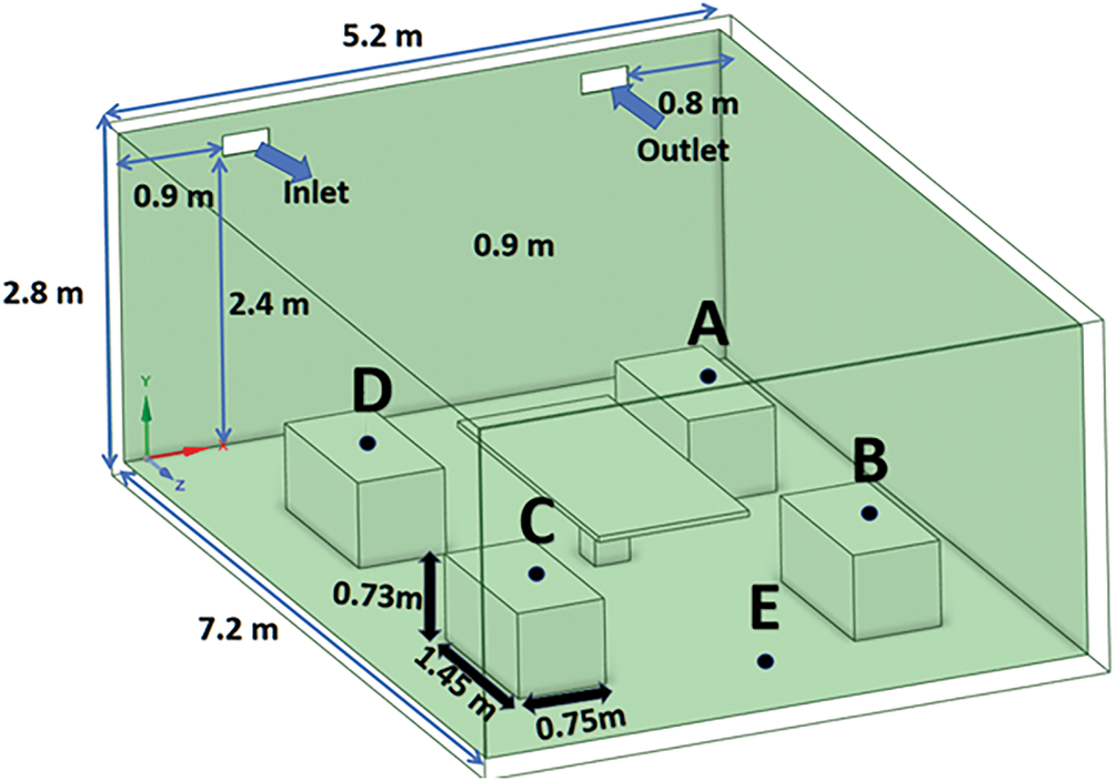
Figure 1: Schematic of the office-like enclosure with desks and exhalation source

As shown in Fig. 2, inside the room, there are four standard office desks (1.45 m × 0.75 m × 0.73 m), and a central table (2.8 m × 1.3 m, thickness 0.05 m). The designated positions A (1.425, 0, −1.475), B (1.425, 0, 1.8), C (−1.475, 0, 1.8), and D (−1.475, 0, −1.375) correspond to the center points of the four standard desks. The global coordinate system is centered at (0, 0, 0), with the heater positioned at (0, 0, 3.2). To model a localized contaminant source, one occupant is designated as releasing exhaled air containing elevated CO2 and aerosols, analogous to a mild respiratory infection scenario. This exhalation is represented by a short cylindrical pipe of 1 cm diameter, extending 0.45 m vertically above the desk surface. The exhalation velocity is set to 0.4 m s−1 at 310 K to reflect slightly warmer human breath.

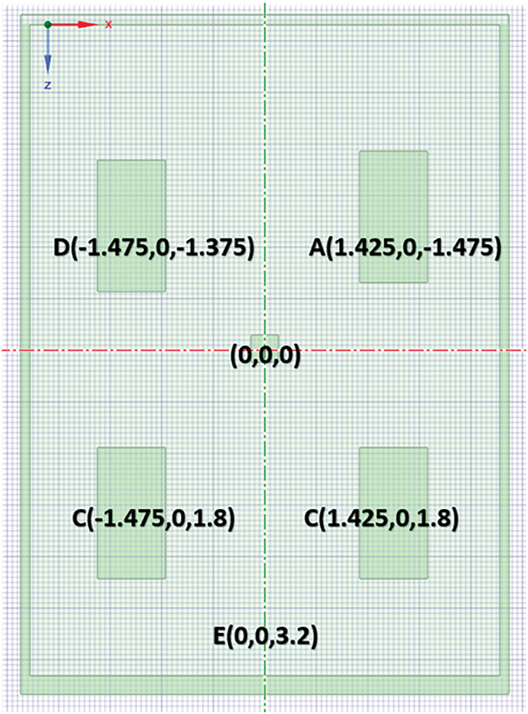
Figure 2: Top view of the enclosure showing desk positions and coordinate system

All walls, the floor, and the ceiling were set to a uniform temperature of 300 K and treated with no-slip boundary conditions. The initial CO2 concentration was 400 ppm, while the exhaled air introduced a higher mass fraction (0.04) to represent a localized contaminant source. Humidity effects and radiative heat transfer were neglected to simplify the model, allowing a realistic yet manageable representation of typical office ventilation scenarios.

2.2 Computational Setup

All simulations are performed using the commercial CFD code ANSYS Fluent [46] in steady-state mode, assuming incompressible turbulent flow. The governing equations are the Reynolds-averaged Navier-Stokes equations for mass, momentum, and scalar transport, complemented by an appropriate turbulence closure. Since buoyancy effects were neglected in this study to focus on forced convection (with isothermal boundaries at 300 K and minimal temperature differences), the continuity equation reads:

∇⋅v=0(1)

where v is the velocity field. The momentum equation takes the form:

ρ(v⋅∇)v=−∇p+∇⋅(µ∇v)+∇⋅(−ρv′v′¯)(2)

Here ρ is air density, µ the dynamic viscosity, p the pressure, and v′v′¯ represents the Reynolds stress tensor. The Buoyancy force was set to 0, as no buoyancy was considered (Boussinesq approximation not applied).

For the pollutant transport (e.g., carbon dioxide), the species conservation equation in Reynolds-averaged form is expressed as:

ρ(v⋅∇Y)=∇⋅(ρDeff∇Y)+SY(3)

where Y is the mass fraction of CO2, Deff is the effective diffusion coefficient (including eddy diffusivity), and SYS is any volumetric source from the exhalation region. SYS = 0.04 (CO2 mass fraction) at the exhalation pipe to represent the breathing plume, and SYS = 0 elsewhere.

To capture flow turbulence, a realizable k-ε model is adopted, as it is widely recognized for its reliability in enclosed, recirculating flows. This model provides transport equations for the turbulent kinetic energy (k) and its dissipation rate (ε). In compressed form:

ρ(v⋅∇k)=∇⋅[(µ+µtσk)∇k]+Gk−ρε(4)

ρ(v⋅∇ε)=∇⋅[(µ+µtσε)∇ε]+ρC1ε−ρC2ε2k+νε(5)

where Gk denotes the production of turbulent kinetic energy, µt is the eddy viscosity, and σk, σε, C1, and C2 are empirical constants. This model was selected after testing alternatives (k-ε RNG and SST k-ω), as it balanced accuracy and efficiency for indoor flows with obstacles (as discussed in Section 3.3).

Since viral aerosols are characterized by particle diameters often below 10 µm, a Discrete Phase Model (DPM) is incorporated to track their trajectories in a Lagrangian framework.

Particles are injected at the exhalation pipe with a specified size distribution. Their motion follows:

dvpdt=v−vpτp+g(ρp−ρ)ρp(6)

where vp is the particle velocity, v is the fluid velocity, ρ is the particle density, and τp is the particle relaxation time. Collisions with walls, inertial impaction, and gravity settling are also taken into account. The Discrete Random Walk (DRW) model was enabled to account for the effect of turbulence on particle diffusion, ensuring realistic stochastic behavior in turbulent flows.

A body-fitted, multi-block hexahedral grid was adopted to curb numerical diffusion in the essentially orthogonal domain. Local refinement was introduced at the supply and return apertures, around desk edges, and along the breathing jet: cell widths of 3 mm at the orifice, 15 mm near the diffusers, and 40 mm in the core volume were successively evaluated, after which further densification produced no discernible change in the monitored variables. Momentum, turbulence and passive-scalar transport were discretised with second-order upwind differencing, while pressure and velocity were linked through the SIMPLE algorithm.

The inflow was prescribed as a uniform velocity profile with magnitudes of 0.7, 1.4, and 2.1 m s−1, turbulence intensity of 5%, and turbulent-to-molecular viscosity ratio of 10 (based on standard indoor airflow assumptions for reproducibility). The outlet was held at atmospheric pressure (101 325 Pa) with zero-gradient conditions for scalars, and the same turbulence parameters as the inlet to ensure symmetrical treatment. All enclosing surfaces were treated as no-slip, isothermal walls at 300 K.

Three inlet speeds—0.7, 1.4 and 2.1 m s−1—were selected to represent 0.5, 1.0 and 1.5 times the reference ventilation rate. Convergence was accepted when residuals for all equations fell below 10−5 and the domain-averaged CO2 mass fraction varied by less than 0.1 % over 500 iterations.

This configuration isolates the interaction of forced convection with internal obstructions and a buoyant contaminant source, allowing detailed maps of air age, CO2 concentration and aerosol loading to be assembled for subsequent IAQ and comfort assessment. Calculations were carried out in ANSYS Fluent 2023 R2 [46] using the pressure-based segregated solver, an approach well suited to the low-Mach, incompressible regime that typifies indoor airflow under steady operating conditions.

2.3 Grid and Mesh Configuration, Independence Study, and Uncertainty Analysis

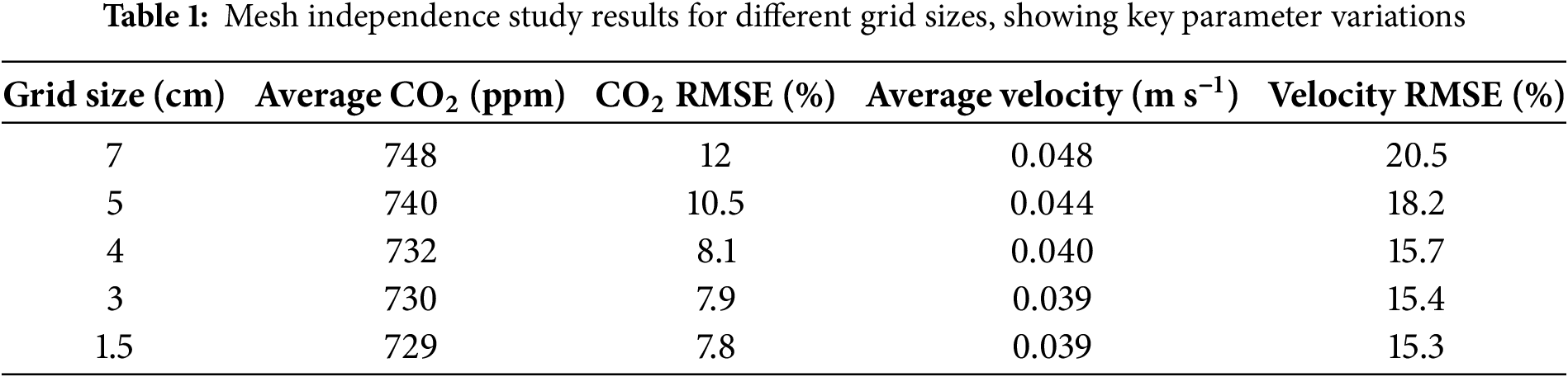
A structured hexahedral mesh was generated to ensure computational accuracy and efficiency. The choice of a structured grid allowed for better alignment with the room geometry and reduced numerical diffusion. The mesh underwent a thorough grid independence study, where grid sizes of 1.5, 3, 4, 5, and 7 cm were tested. The specific results are presented in Table 1, showing variations in average CO2 concentration, airflow velocity, RMSE values, and computational time across the tested grids. As shown, the 4 cm grid achieves convergence with less than 3% variation in key parameters compared to finer grids, providing a balance between computational cost and result accuracy.

For regions with higher gradients, such as the breathing simulation pipe, finer grids with a resolution of 3 mm were employed to capture detailed flow and pollutant dynamics. Similarly, the inlet and outlet boundaries were refined using a 1.5 cm mesh to ensure accurate representation of flow development and pollutant entrainment.

Boundary layer refinement was applied using prism layers to adequately resolve near-wall regions. Specifically, 10 prism layers with a growth rate of 1.2 were used, a standard configuration for k-ε turbulence models in indoor airflow simulations to ensure proper boundary layer coverage. The area-weighted average non-dimensional wall distance (Y+) was maintained at 3.5 in the Enhanced Wall Treatment (EWF) model, as this value falls within the recommended range of 1-5 for EWF, enabling accurate wall function application and blending between viscous sublayer and log-law regions without requiring excessive mesh refinement or computational resources. This approach ensured accurate representation of boundary layer phenomena while maintaining computational efficiency.

Air, Carbon Dioxide, and Aerosol Settings

Airflow was initialized with three ventilation speeds of 0.7, 1.4, and 2.1 m s−1 at the inlet, with an inlet temperature of 300 K. The outlet was set to atmospheric pressure, ensuring consistent ventilation flow throughout the room. Carbon dioxide was modeled as a passive scalar, introduced at the breathing pipe with a mass fraction of 0.04 and at the inlet with a mass fraction of 0.006. These values were derived from validation data and supported by relevant literature.

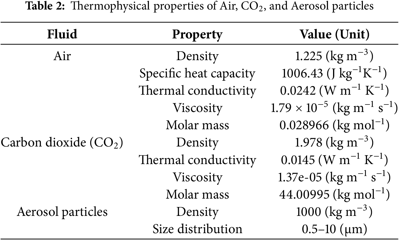
The specific thermophysical properties for air, CO2, and aerosol particles—such as density, viscosity, and thermal conductivity—were defined based on validation data and relevant literature, ensuring a realistic representation of occupant respiration and typical indoor conditions. Table 2 summarizes the key properties used in the simulations.

Aerosol particles were modeled using the Discrete Phase Model (DPM) with a Lagrangian approach to track individual particle trajectories. The six aerosol size classes (0.5, 1, 3, 5, 7, 10 µm) were chosen to represent a polydisperse distribution typical of respiratory emissions, covering sub-micron particles that remain airborne and larger ones prone to rapid settling, based on literature on viral aerosol dynamics where small particles dominate by number and larger by mass (e.g., Wells [47] and COVID-19 droplet measurements [48]). The particle size distribution and mass flow rates are detailed in Table 3.

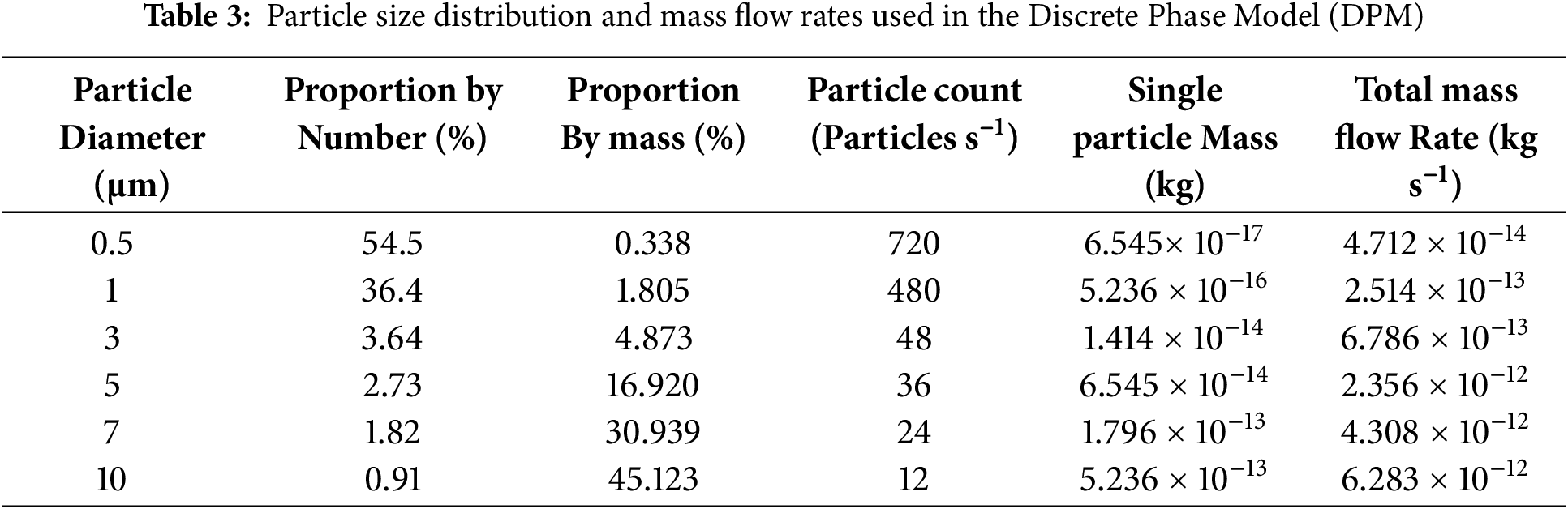
The particles were injected through the breathing pipe, modeled as a surface source with a velocity of 0.4 m s−1 and a temperature of 310 K. Particle interactions with the airflow, gravity, and wall collisions were considered, and sedimentation effects were accounted for using Stokes’ law.

τp=ρpdp218µ(7)

The gravitational settling velocity of viral aerosols was estimated using Stokes’ Law, which describes the settling behavior of small spherical particles in a fluid. The terminal velocity (Vt) of a particle under gravity is given by the following equation:

Vt=(ρp−ρ)gdp218µ(8)

where ρp is the particle density (1000 kg m−3 for biological aerosols), ρ is the air density (1.225 kg m−3 at 300 K), g is the gravitational acceleration (9.81 m s−1), dp is the particle diameter, and µ is the dynamic viscosity of air (1.8 × 10−5 kg/m s).

The Stokes’ number (Stk) was also evaluated to determine the inertial behavior of the particles in response to airflow changes. The Stokes’ number is given by the following equation:

Stk=ρpdp2U18µL(9)

where U is the characteristic flow velocity and L is a characteristic length scale (e.g., the inlet or obstruction scale in the domain). A low Stokes number (Stk < 1) indicates that particles closely follow the airflow streamlines, while a higher Stokes number (Stk > 1) suggests that particles exhibit significant inertia and may deviate from the streamlines.

In ANSYS Fluent, particle gravitational settling was incorporated by enabling the gravity option in the Discrete Phase Model (DPM). The terminal velocity predicted by Stokes’ law was compared with the Fluent simulation results to validate the accuracy of the model. This comparison ensures that aerosol dispersion and sedimentation are accurately captured in the computational domain.

This approach ensured accurate representation of boundary layer phenomena while maintaining computational efficiency. A schematic diagram of the mesh is presented in Fig. 3, illustrating the overall structured hexahedral grid, local refinements (e.g., 3 mm at the exhalation source, 1.5 cm at inlet/outlet), and boundary layer details. The total mesh consists of 6,088,891 elements and 1,170,003 nodes, as shown in the figure.

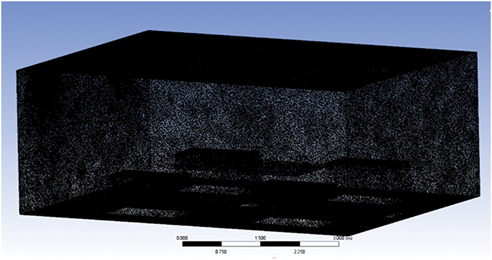
Figure 3: Schematic of the structured hexahedral mesh with local refinements (3 mm at exhalation source, 1.5 cm at inlet/outlet), prism layers (Y+ = 3.5), and totals (6,088,891 elements; 1,170,003 nodes)

2.4 Solver and Numerical Settings

The pressure-velocity coupling was addressed using the Rhie-Chow algorithm, a momentum-based method suitable for maintaining stability in incompressible flow simulations. For spatial discretization, a least squares cell-based approach was employed for pressure, while second-order upwind schemes were applied to the momentum, CO2, and energy equations to enhance accuracy and reduce numerical diffusion in regions with steep gradients. The turbulent kinetic energy and dissipation rate were discretized using first-order upwind schemes to ensure computational efficiency. These settings were carefully selected to optimize both simulation accuracy and efficiency, ensuring reliable results for the indoor airflow and pollutant dispersion analysis.

2.5 Age of Air

The age of air was calculated to assess the ventilation efficiency of the indoor space by determining how long air particles had remained within the room. A passive scalar transport approach was used, where each cell’s mean residence time was computed based on cumulative airflow trajectories from the inlet. This approach allows for the visualization of zones with prolonged air recirculation. Such areas are often associated with stagnant air, where pollutants can accumulate.

The age of air is an important metric for identifying regions within a room that might have lower ventilation effectiveness. By mapping the age of air, we can pinpoint areas requiring improvements in airflow or ventilation design.

Here, ϕ represents the scalar air age, Γ is the diffusion coefficient, and Sϕ is the source term. Sϕ = 1 s−1 throughout the domain, representing the uniform aging of air parcels as they reside in the space (standard in age-of-air calculations).

ρ(v⋅∇ϕ)=∇⋅(Γ∇ϕ)+Sϕ(10)

The diffusion coefficient, Γ, is defined as:

Γ=µ+µtSct(11)

This formulation enabled the identification of regions with high air age, which are indicative of poor ventilation performance. By analyzing the spatial distribution of air age, the effectiveness of various ventilation speeds could be assessed.

The numerical set-up follows the measured operating envelope as closely as practicable while retaining computational economy. The supply diffuser delivers air at three nominal speeds—0.7, 1.4 and 2.1 m s−1—representing 0.5, 1.0 and 1.5 times the reference velocity recorded during the validation trials. Turbulence at the inlet is prescribed with an intensity of 5% and a turbulent-to-molecular viscosity ratio of 10. The supply temperature is fixed at 300 K so that the influence of flow rate can be examined independently of buoyancy effects. The return grille is maintained at atmospheric pressure (101,325 Pa) and assigned the same turbulence parameters as the inlet to ensure a symmetrical treatment of the Reynolds stress field.

The breathing orifice, which mimics a seated occupant, issues a jet at 0.4 m s−1 and 310 K. The exhaled mixture contains 4% CO2 by mass and a six-class aerosol ensemble distributed as 0.5 µm (54.5%), 1 µm (36.4%), 3 µm (3.64%), 5 µm (2.73%), 7 µm (1.82%) and 10 µm (0.91%) by number. Particle density is taken as 1000 kg m−3, and the carrier-gas viscosity is 1.8 × 10−5 kg m−1 s−1, values that reproduce the settling and response times predicted by Stokes theory. Mass-flow rates for each diameter class were pre-computed to match the prescribed number fractions and entered directly into the Discrete-Phase module of ANSYS Fluent.

All solid boundaries (walls, floor, ceiling, furniture) are treated as no-slip, isothermal surfaces held at 300 K. Omitting sensible heat release from occupants (≈65 W m−2) limits the study to forced-convection phenomena; future work will relax this simplification to quantify buoyancy-momentum coupling. The domain is initialised at 300 K and 400 ppm CO2 to provide a uniform baseline.

These boundary choices—together with the Realisable k-ε closure—have been adopted in earlier indoor-air studies for low-Mach, incompressible regimes and are consistent with the experimental conditions described in Section 3 [49].

To ensure the reliability and accuracy of the CFD simulation, we conducted a comprehensive mesh independence study and model uncertainty analysis (detailed results in Table 1 of Section 2.3). The computational domain was meshed using a structured hexahedral mesh with fine resolution near key areas, including the inlet/outlet, breathing zone, and near-wall region. A total of five mesh sizes (7, 5, 4, 3, and 1.5 cm) were evaluated to determine the optimal mesh resolution. The results showed that the variation in key output parameters (such as average CO2 concentration and airflow velocity at the monitoring point) between 4 and 3 cm meshes was less than 3%. In addition, the results such as contour plots and flow patterns were consistent for these mesh sizes, confirming the mesh independence at 4 cm resolution.

The simulation establishes convergence criteria by monitoring the residuals of all governing equations, including momentum, continuity, turbulence, energy, species transport, and discrete phase tracking. The simulation results are considered converged when the residuals are below 10−5 and the monitored variables exhibit less than 0.5% variation over 500 iterations.

Several uncertainties were considered during the modeling process:

First is geometric simplification: our simulations assume that furniture and surfaces have ideal geometry. In reality, complex shapes and surface textures may affect the flow of gases.

Steady-state assumption: the simulations are performed under steady-state conditions, but the thermal plume caused by human breathing and occupancy is transient in nature. Current methods may not capture the temporal variation of pollutant dispersion.

CO2 emission rate: we use a fixed exhaled CO2 mass fraction of 0.04. However, real breathing exhibits variations in both frequency and volume, introducing uncertainties in pollutant loading.

Aerosol emission: we model only one exhalation source, while there are typically four people in the lab. This simplification is intentional in order to focus on the detailed analysis of particle trajectories and suspension times, preventing the influence of other pollution sources. Similar simplifications have been used in related studies to isolate specific variables in the analysis of pollutant dispersion.

3  Validation

3.1 Experimental Setup

To validate the computational fluid dynamics (CFD) simulations, a series of wind speed and CO2 concentration measurements were conducted in a real office environment. The chosen office is a typical workspace used for research activities, featuring a rectangular layout with a single air inlet and outlet, two windows, an electric radiator, multiple desks, and storage cabinets. These elements play a crucial role in influencing the indoor airflow patterns.

The experimental measurements were taken between late June and early July, a period marked by atypical climatic conditions, with outdoor temperatures ranging from 15∘C to 25∘C and windy conditions. These external environmental factors likely affected indoor air quality and ventilation dynamics, making this study period especially relevant for analyzing air exchange efficiency.

3.1.1 Geographical and Structural Characteristics of the Experimental Room

The experimental room measures 7.2 m × 5.2 m × 2.8 m and is typically occupied by four doctoral students, each contributing thermal emissions of approximately 65 W/m2, due to activities like typing on keyboards.

Airflow in the room is mainly controlled by a single air inlet and outlet, in addition to two north-facing windows (1.3 m × 0.98 m) and an electric radiator placed beneath the windows. The room is furnished with five large desks and additional smaller tables for student use. Four of the major desks are positioned at the corners of the room, while a fifth desk is centrally located (see Fig. 4). The presence of these furniture elements significantly influences air circulation and pollutant dispersion within the space.

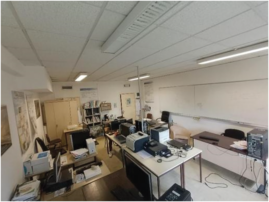
Figure 4: Interior view of the experimental room

3.1.2 Measurement Equipment and Sensor Configuration

For experimental validation, the ALMEMO 2690 device was used to monitor and record essential environmental parameters such as air velocity, temperature, and humidity. This device is ideal for applications that require high-precision, simultaneous measurements of multiple environmental variables.

The ALMEMO 2690 system allows for modular connectivity with various sensors. In this study, sensors dedicated to temperature, relative humidity, and air velocity were used to gather precise real-time data. This measurement system ensures high accuracy, guaranteeing reliable environmental monitoring. The wind speed meter used in this study is depicted in Fig. 5.

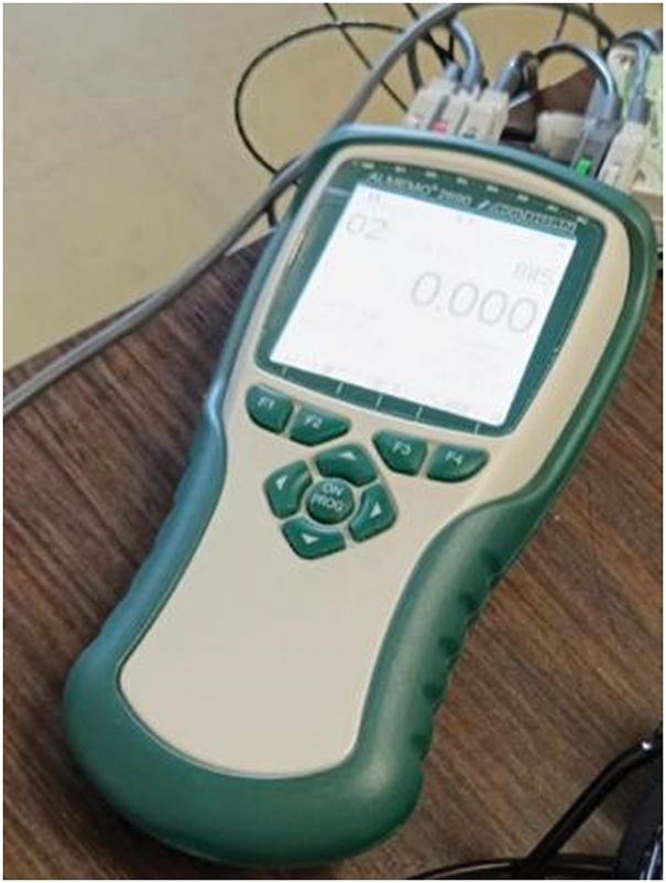
Figure 5: ALMEMO 2690

The collected data was stored in the internal memory of the device for post-processing and subsequently exported to a computer for detailed analysis. This streamlined workflow facilitated an efficient evaluation of indoor air dynamics and ventilation performance. To quantify measurement uncertainty, the air velocity sensor has an estimated uncertainty of ±0.01 m s−1 (approximately 2% relative error), while the CO2 sensor has ±50 ppm (approximately 5% relative error), based on the ALMEMO 2690 specifications and standard calibration procedures.

3.1.3 Experimental Measurement Points and CO2 Monitoring

The airflow velocity measurements were taken at multiple points corresponding to locations within the CFD simulation, enabling a direct comparison between experimental and numerical results. As shown in Fig. 6, five measurement points (A–E) were strategically positioned within the room. Wind speed and CO2 concentration were measured at two heights (1.1 and 1.5 m) for locations A–D, while point E was monitored at a single height of 1.5 m. These measurement locations were carefully selected to capture key airflow characteristics in critical zones of the room.

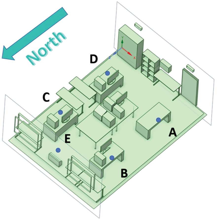
Figure 6: Measurement points (A–E) for airflow velocity and CO2 concentration monitoring in the experimental room

Wind Speed Measurements: The experimental wind velocity at the air inlet was recorded as 1.37 m s−1, which slightly differed from the simulation values of 0.7, 1.4, and 2.1 m s−1 used in the computational analysis.

CO2 Concentration Measurements: The initial CO2 concentration before the experiment was 355 ppm, with continuous monitoring carried out at designated locations throughout the experiment.

The precise placement of the CO2 sensors was aligned with the four major desks (A, B, C, D), ensuring comprehensive coverage of pollutant dispersion patterns. Data collection points for both air velocity and CO2 concentrations were strategically positioned to capture areas of airflow stagnation and circulation effects.

3.1.4 Experimental Boundary Conditions and Data Processing

To ensure consistency with the CFD model, the experimental boundary conditions were defined as follows:

The air inlet velocity was measured at 1.37 m s−1.

Rather than maintaining a constant room temperature of 300 K, temperature data were collected from various surfaces within the room to provide realistic thermal boundary conditions for the Fluent simulations.

The CO2 emissions were derived from normal human occupancy, resulting in an inherently variable emission rate that contributed to notable discrepancies between the simulation predictions and the experimental data.

The experimental measurements were subsequently analyzed using RMSE and R2 metrics, offering an objective means to assess the level of agreement between the CFD results and the observed airflow and pollutant dispersion. No filtering or anomaly correction was applied to the CO2 data.

3.2 Validation Metrics

The validation of numerical simulations necessitates the use of robust statistical measures to quantify the agreement between experimental observations and computational predictions. In this study, two primary validation metrics were adopted: the Root Mean Square Error (RMSE) and the coefficient of determination (R2). These indices serve as essential indicators of the predictive accuracy and reliability of the computational fluid dynamics (CFD) model.

3.2.1 Root Mean Square Error (RMSE)

The RMSE is a widely utilized metric that quantifies the average deviation between experimental and numerical results. It is particularly sensitive to large deviations and thus provides a rigorous assessment of simulation fidelity. The RMSE is calculated as follows:

RMSE=1n∑i=1n(Xexp,i−Xsim,i)2(12)

where Xexp,i and Xsim,i denote the experimentally measured and simulated values, respectively, at observation point i, and n represents the total number of measurements. A lower RMSE indicates better agreement between the simulation and experimental data, while higher values suggest significant discrepancies.

In the context of this study, RMSE was computed for both air velocity and CO2 concentration at various locations within the experimental domain. Given the dynamic nature of indoor airflow and the inherent variability of human-generated CO2 emissions, the RMSE serves as a critical parameter for assessing the model’s ability to replicate real-world conditions.

3.2.2 Coefficient of Determination (R2)

The coefficient of determination (R2) is a statistical measure that evaluates the strength and direction of the linear relationship between simulated and experimental results. It is expressed as:

R2=1−∑i=1n(Xexp,i−Xsim,i)2∑i=1n(Xexp,i−X¯exp)2(13)

where X¯exp represents the mean of the experimental observations. The R2 value ranges between 0 and 1, where values closer to 1 indicate a high degree of correlation between numerical and experimental data, signifying a well-calibrated model.

In this study, R2 values were determined for airflow velocity and CO2 concentration across different measurement points. A strong correlation (R2 > 0.85) would suggest that the CFD model captures the dominant physical processes governing indoor airflow and contaminant dispersion.

3.2.3 Justification for Selected Metrics

The selection of RMSE and R2 is based on their complementary nature. While RMSE offers an absolute measure of deviation, R2 provides a relative assessment of how well the numerical predictions align with observed trends. Together, these metrics deliver a comprehensive evaluation of the model’s performance, facilitating both localized error assessment and global pattern recognition.

Furthermore, the interpretation of these metrics must account for potential sources of uncertainty, such as sensor precision, environmental fluctuations, and variations in human activity within the experimental space. Since CO2 emissions were influenced by natural breathing patterns, some deviations between the numerical and experimental results were expected.

By incorporating these validation metrics, this study ensures a thorough evaluation of the CFD model’s predictive capability. This approach enhances the credibility of the simulation results and reinforces their applicability in optimizing indoor ventilation strategies.

3.3 Comparison with Experimental Data

To assess the accuracy of the CFD simulations, experimental measurements of air velocity and CO2 concentration were conducted at multiple locations within the validation room. To reassure numerical accuracy, a grid independence study was performed (detailed in Section 2.3 and Table 4), confirming that the selected 4 cm mesh provides convergence with less than 3% variation in key parameters compared to finer grids.

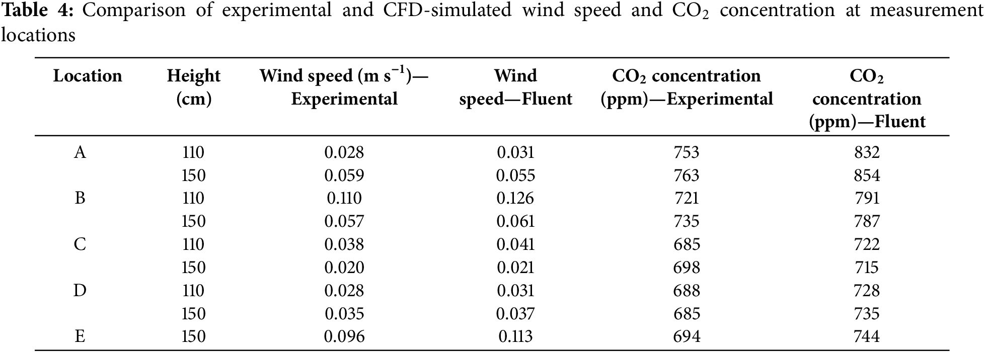
The comparison between numerical predictions and experimental data provides critical insights into the model’s capability to replicate real-world indoor airflow and pollutant dispersion.

The validation process involved collecting wind velocity and CO2 concentration data at five selected points (A–E), measured at two heights (1.1 and 1.5 m) where applicable. The measured airflow velocity at the inlet was 1.37 m s−1, which corresponds to the mid-range value used in the numerical simulations (0.7, 1.4, and 2.1 m s−1). The CO2 concentration prior to the experiment was recorded at 355 ppm, ensuring that the relative increase in CO2 levels due to occupant emissions could be effectively compared between experimental and numerical results.

The results for CO2 concentration show a reasonable agreement between the simulations and experimental measurements. However, numerical predictions tend to slightly overestimate CO2 levels, particularly at positions A (110 cm) and B (110 cm), where discrepancies between measured and simulated values reached 79 ppm and 70 ppm, respectively. This overestimation is likely due to the model’s assumption of a constant CO2 release rate, whereas human respiration naturally occurs in cycles, leading to fluctuations in emissions.

Despite these discrepancies, the general trend of CO2 dispersion was accurately captured by the numerical model. The predicted spatial distribution of CO2 aligns well with the experimental observations, with higher concentrations near the emission source and gradual dilution towards the room’s ventilation outlets.

Given the complex airflow dynamics within the room, several turbulence models were tested to identify the most suitable approach for simulating indoor airflow and pollutant dispersion. Three models were considered: k-ε RNG, k-ε Realizable, and SST k-ω. The comparison showed that both k-ε Realizable and SST k-ω models provided satisfactory predictive capabilities, accurately capturing key features of air movement and pollutant transport.

Ultimately, the k-ε Realizable model with Enhanced Wall Function (EWF) was selected for its superior balance between computational efficiency and accuracy. This model is widely validated for indoor airflow applications, handling both large-scale turbulent structures and near-wall effects in ventilated spaces effectively. The selection was further supported by its ability to maintain a strong correlation between simulated and experimental results, as indicated by the high R2 value.

While the validation results demonstrate the model’s capacity to predict airflow and CO2 dispersion, certain sources of uncertainty must be acknowledged:

Measurement Accuracy: The ALMEMO 2690 device, though highly precise, has inherent sensor limitations that could contribute to minor deviations in recorded values.

Environmental Variability: External factors such as slight fluctuations in room pressure, temperature variations, and airflow disturbances caused by occupants could introduce experimental inconsistencies.

Human-Induced Variability: The simulation assumes a steady CO2 emission rate, while actual human respiration fluctuates over time, adding natural variability to the experimental measurements.

Overall, the validation process confirms that the CFD model reliably represents indoor airflow and pollutant transport. The chosen k-ε Realizable EWF turbulence model ensures that the numerical simulations closely align with real-world observations, reinforcing the model’s applicability for future studies on ventilation optimization and indoor air quality assessment.

4  Results and Discussion

4.1 Comparison of Virus Particle Trajectories

Understanding the dispersion behavior of viral aerosols in indoor environments is crucial for assessing exposure risks and optimizing ventilation strategies. To link these findings to practical design, we further analyzed how ventilation rates alter particle residence time and potential exposure hotspots, providing targeted recommendations for ventilation layout. This study investigates the trajectories of virus particles with different diameters (0.5–10 µm) within an airflow field, focusing on their movement patterns, suspension characteristics, and deviation from the primary airflow trajectory.

4.2 Particle Size and Deviation from Airflow Trajectories

Fig. 7 compares gas pathlines and virus particle trajectories (0.5 µm diameter) at a ventilation velocity of 0.7 m s−1. The visualization highlights the similarity between particle trajectories and gas flow, reflecting the minimal influence of gravitational forces on small particles. Simulation results indicate that smaller particles (0.5 and 1 µm) closely follow the airflow, exhibiting minimal deviation. Fig. 7 clearly illustrates this behavior, showing virus particle trajectories nearly overlapping with gas pathlines due to their lower inertia. These small particles remain suspended longer, significantly increasing their potential for airborne transmission, especially in regions with poor ventilation. Due to their reduced gravitational settling, these aerosols spread widely, underscoring the need for efficient ventilation systems to prevent accumulation in poorly ventilated zones.

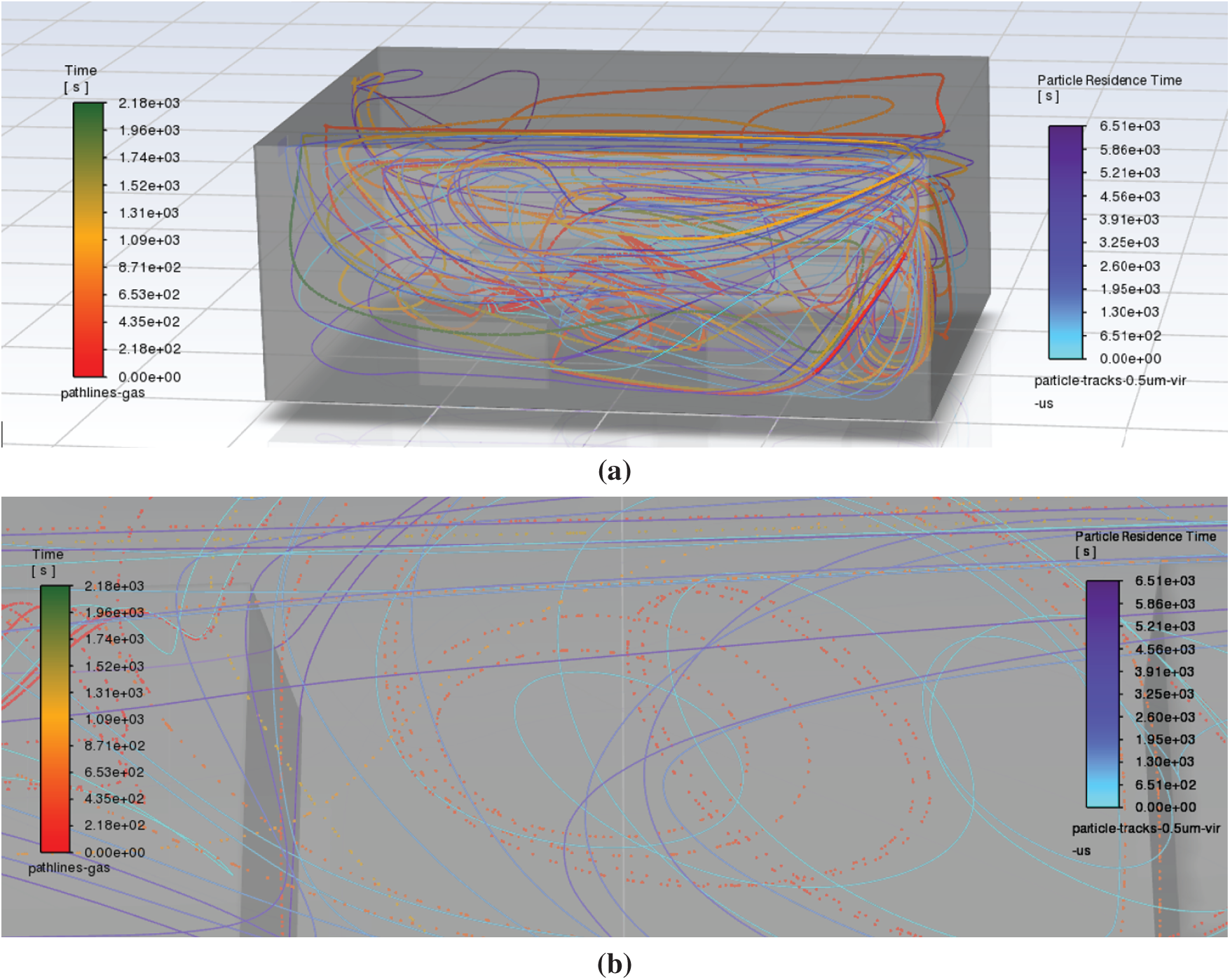
Figure 7: Comparison of gas pathlines (points) and virus aerosol trajectories (lines, 0.5 µm diameter) at ventilation velocity of 0.7 m s−1: (a) Overall distribution; (b) Enlarged local view near the emission source

Due to their smaller size and lighter mass, these particles do not easily settle under gravitational forces, instead remaining airborne for longer durations, which increases their likelihood of inhalation and transmission. In indoor environments with inadequate ventilation, these particles can accumulate and disperse over a wide area, increasing the exposure risk for occupants. This behavior emphasizes the importance of optimizing ventilation rates to minimize particle accumulation in areas of limited airflow.

As shown in Fig. 8, increasing the particle diameter decreases the relative influence of drag forces while amplifying the effect of gravity, leading to a more pronounced downward displacement. This deviation becomes especially evident for particles larger than 5 µm, which exhibit shorter transport distances and a more localized dispersion pattern.

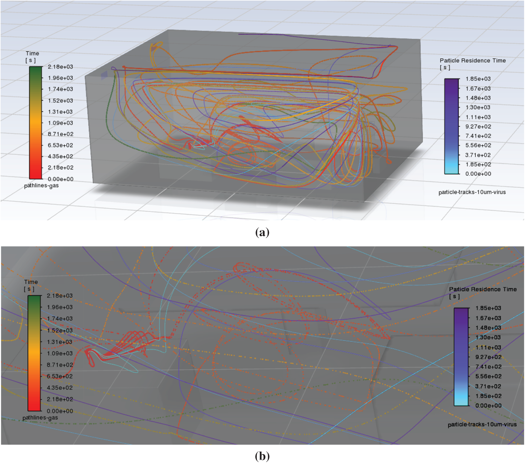
Figure 8: Comparison of gas pathlines (points) and virus aerosol trajectories (lines, 10 µm diameter) at ventilation velocity of 0.7 m s−1: (a) Overall distribution; (b) Enlarged local view near the emission source

Larger particles, due to their greater mass, experience stronger gravitational forces, causing them to settle more quickly compared to smaller particles. As a result, their suspension time in the air is significantly reduced, limiting their range of travel. This suggests that larger particles are more likely to settle on surfaces, potentially contaminating surrounding areas.

In indoor environments, these larger particles are less likely to remain airborne for extended periods and are more susceptible to local airflow patterns and surface interactions. Therefore, understanding how particle size affects dispersion is crucial for designing effective ventilation strategies that reduce the risk of exposure to both smaller airborne particles and larger particles that may settle and contaminate surfaces. Furthermore, due to their increased mass, these larger particles tend to circulate more slowly within specific regions rather than being widely dispersed by the airflow. This phenomenon may result in the accumulation of contaminants in localized areas, thereby heightening the risk of exposure in those zones, continuing the need for tailored ventilation systems that address both fine and larger particles.

Key Observations and Implications

Small particles (0.5–1 µm): These particles remain primarily suspended in the air, closely following the airflow streamlines with minimal deviation.

Large particles (3–10 µm): These particles exhibit significant deviation from the primary airflow trajectories, settle more rapidly, have a reduced airborne transport range, and tend to accumulate in localized areas.

These findings underscore the critical role of particle size in assessing airborne transmission risks. Smaller particles, due to their extended suspension time in the air, highlight the need for efficient ventilation to reduce their spread. In contrast, while larger particles settle more quickly, they may accumulate in specific regions, raising the risk of localized contamination. Effective ventilation and air purification strategies, tailored to address these distinct dispersion behaviors, are essential for minimizing the potential hazards associated with viral aerosol transmission.

4.3 Particle Suspension and Ventilation Effects

4.3.1 Impact of Particle Size on Suspension Time

The behavior of aerosolized viral particles within an indoor environment is profoundly influenced by their size, as it directly affects their aerodynamic properties and interactions with the surrounding airflow. Fig. 9 illustrates the mean residence time of viral particles of various diameters at an inlet velocity of 0.7 m s−1. The results indicate that smaller particles (0.5–2 µm) remain suspended for extended durations, often exceeding 2000 s, as they closely follow the airflow streamlines with minimal gravitational settling. In contrast, larger particles (greater than 5 µm) exhibit significantly shorter residence times, with a distinct downward drift due to the dominant influence of gravitational settling.

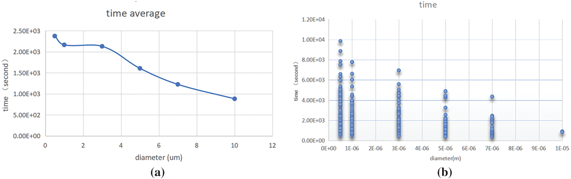
Figure 9: Mean residence time of viral particles at an inlet velocity of 0.7 m s−1: (a) Average residence time as a function of particle diameter, (b) Scatter plot of individual particle suspension times

The range of residence times across different particle sizes is further visualized in Fig. 9, where individual particle trajectories display greater variation for smaller particles. This pattern suggests that, while some finer aerosols may be carried out through the ventilation system, others can persist in recirculating eddies within the room for prolonged periods, further complicating the dynamics of airborne transmission.

4.3.2 Effect of Ventilation Speed on Suspension Time

To assess the influence of ventilation, Fig. 10 shows both the mean and individual residence times of viral particles at an increased airflow velocity of 1.4 m s−1. The results demonstrate a general reduction in suspension times for all particle sizes. Smaller aerosols (0.5–2 µm) continue to exhibit a strong tendency to remain airborne, yet their residence time is reduced by nearly 40% compared to the lower airflow condition. In contrast, particles larger than 5 µm experience a much more significant decrease in residence time, underscoring the effectiveness of ventilation in facilitating their rapid removal from the air.

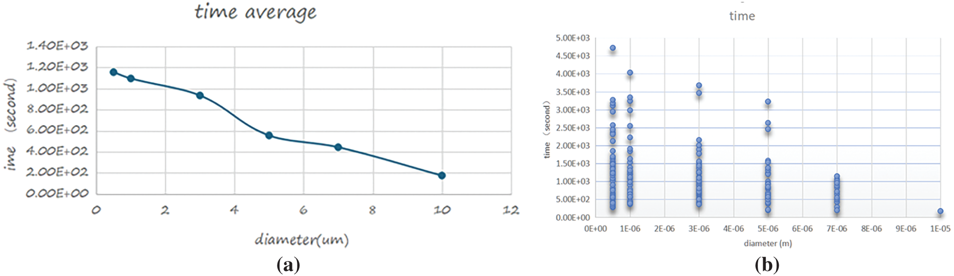
Figure 10: Mean residence time of viral particles at an inlet velocity of 1.4 m s−1: (a) Average residence time as a function of particle diameter, (b) Scatter plot of individual particle suspension times

Further increasing the airflow velocity to 2.1 m s−1 (Fig. 11) leads to a significant reduction in suspension time across all particle sizes. Notably, particles larger than 5 µm are rapidly transported out of the domain, effectively minimizing their concentration in indoor air. However, even at the highest ventilation rate, smaller aerosols continue to exhibit extended residence times, though their overall dispersion is noticeably reduced.

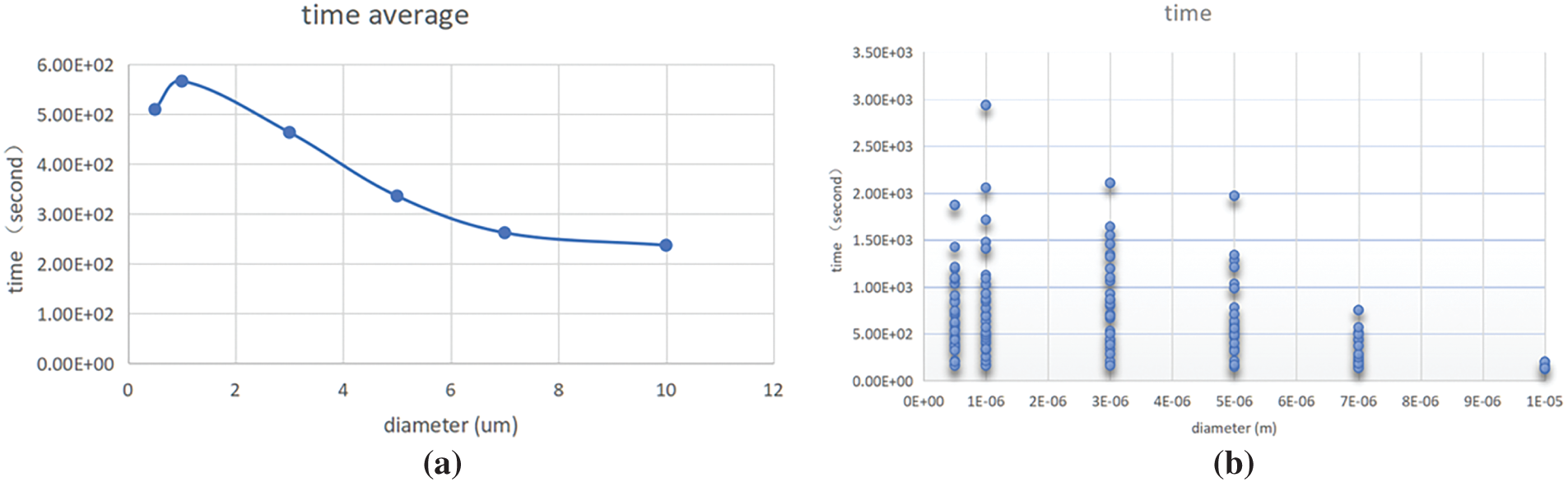
Figure 11: Mean residence time of viral particles at an inlet velocity of 2.1 m s−1: (a) Average residence time as a function of particle diameter, (b) Scatter plot of individual particle suspension times

These findings underscore the pivotal role of ventilation in reducing the persistence of airborne viral particles. While increased airflow effectively shortens the residence time of larger particles, smaller aerosols remain suspended for longer periods. This suggests that a combination of mechanical ventilation and additional mitigation strategies, such as advanced filtration or localized air extraction, may be necessary to optimize indoor air quality and reduce the risk of viral exposure.

Moreover, the results emphasize the need to tailor ventilation rates to the specific characteristics of indoor environments. While higher ventilation speeds are effective at removing larger particles, they may not be sufficient to eliminate fine aerosols entirely. Therefore, implementing a ventilation system that balances efficient airflow with targeted filtration could offer a more comprehensive approach to mitigating airborne transmission risks.

4.4 Differences between CO2 and Virus Dispersion

The dispersion patterns of carbon dioxide (CO2) and viral aerosols differ significantly due to their distinct physical properties and interactions with airflow. Recognizing these differences is crucial for assessing indoor air quality and infection risk.

4.4.1 Spatial Distribution Differences

As a gaseous pollutant, CO2 tends to distribute more uniformly within indoor environments due to its lower density and rapid diffusion. As shown in Fig. 12 (perpendicular to the room), the CO2 concentration forms relatively homogeneous gradients, spreading along airflow paths and quickly reaching equilibrium. In contrast, the mass concentration of viral aerosols under the same conditions exhibits pronounced heterogeneity. Due to their higher mass, viral particles are more likely to accumulate in specific regions, particularly in areas with lower airflow velocities or near surfaces.

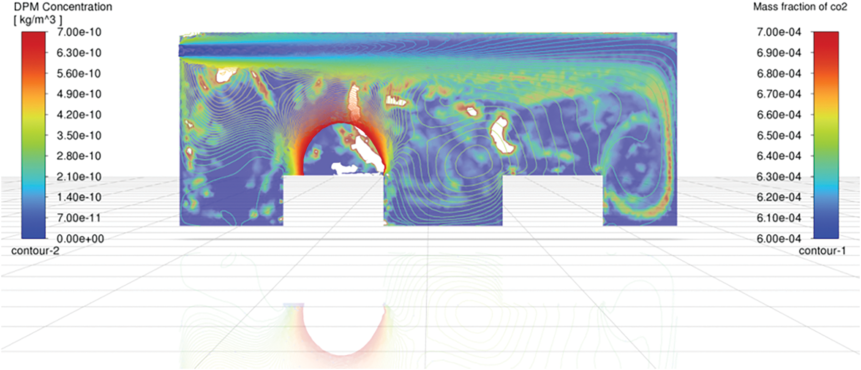
Figure 12: Co-located contours of virus-laden dry particle matter (DPM) mass concentration (left colour bar, kg m−3) and CO2 mass fraction (right colour bar, -) on the vertical mid-plane x = 0.9 m for an inlet velocity of 0.7 m s−1

Similarly, Fig. 13 (parallel to the floor) further highlights the differences between CO2 and viral aerosol dispersion. While CO2 maintains a relatively uniform diffusion pattern, viral particles form localized high-concentration zones, particularly within recirculating airflow regions. This observation underscores the significant role of gravitational settling and inertial effects in viral dispersion, setting their behavior apart from gaseous pollutants.

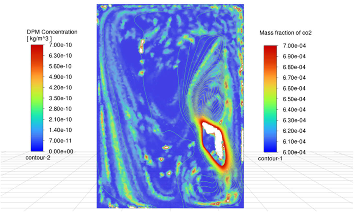
Figure 13: Co-located contours of virus-laden dry particle matter (DPM) mass concentration (left colour bar, kg m−3) and CO2 mass fraction (right colour bar, -) on the horizontal plane y = 1 m for an inlet velocity of 0.7 m s−1

4.4.2 Key Findings

CO2 dispersion tends to be largely homogeneous, making it a useful indicator for assessing ventilation efficiency. However, its uniform distribution does not directly correlate with the dispersion of viral aerosols. Unlike CO2, viral particles tend to accumulate in specific zones, especially where airflow is weaker or near surfaces, thereby increasing the risk of localized exposure. The divergence shows that neither CO2 level nor mean age of air, taken in isolation, delineates all high-exposure zones. We therefore recommend that ventilation design be informed by a composite diagnosis that couples gas data, size-resolved particle measurements, and rapid CFD appraisal.

4.5 Limitations of Using Air Age as a Contamination Indicator

Air age is widely used as an indicator of ventilation efficiency and indoor air quality, providing insights into the average time air has spent within a given space. However, its effectiveness in predicting the dispersion of airborne contaminants, particularly virus-laden aerosol particles, has significant limitations. This study evaluates air age as a proxy for contamination risk and highlights discrepancies between air age distribution and actual particle accumulation patterns. Fig. 14 presents the spatial distribution of air age alongside the mass concentration of virus-laden particles (1.476409e–10 kg m−3 isosurface).

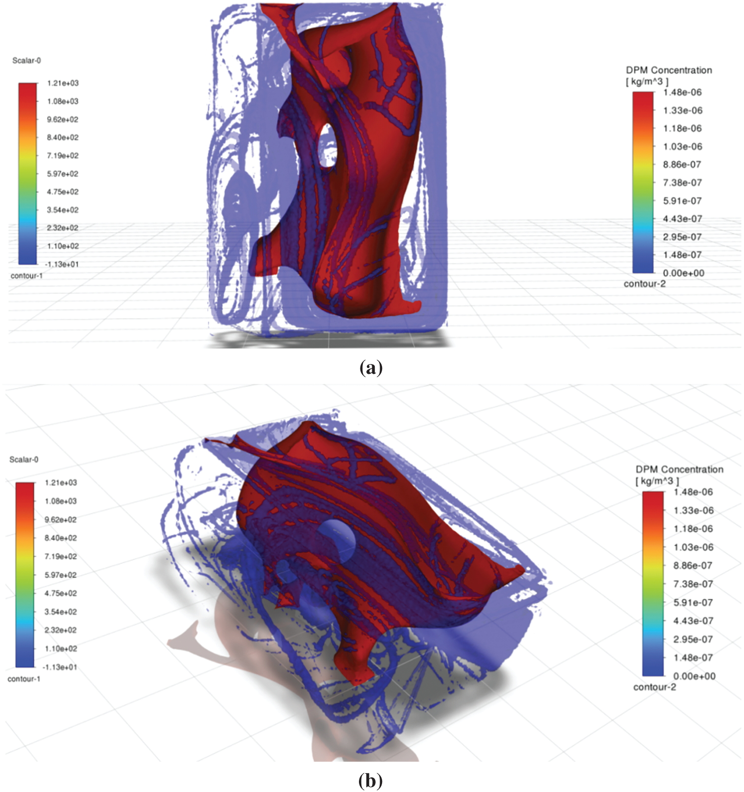
Figure 14: Iso-surfaces of (red) air age τ>1200 s and (blue) virus-laden aerosol mass concentration C > 1.47 × 10−7 kg m−3: (a) Top (plan) view; (b) Main (front-isometric) view

The results reveal a fundamental mismatch between air age and viral accumulation patterns. While the highest air age values are observed in the central region of the room, the concentration of virus particles is notably higher near the walls. This finding suggests that stagnant air does not necessarily correlate with areas of increased contamination risk. Instead, viral aerosols tend to accumulate in regions influenced by airflow recirculation and gravitational settling, phenomena that air age metrics fail to adequately capture.

The observed discrepancies indicate that air age alone cannot reliably predict areas of elevated contamination risk. Several factors contribute to this limitation. First, air age measures the time since the air last entered the room but does not account for the transport dynamics of particulate pollutants, which are influenced by inertia, turbulence, and gravitational settling. Second, air age assumes homogeneous mixing of pollutants, an assumption that does not hold for virus aerosols, which exhibit complex dispersion behaviors driven by factors such as particle size, density, and airflow patterns.

Given these limitations, relying solely on air age to evaluate airborne contamination risk may result in underestimating or misinterpreting high-risk areas. While air age remains a valuable metric for assessing ventilation effectiveness, it should be complemented by additional indicators, such as direct measurements of particle concentration and localized airflow patterns. In future work, air age could be combined with other indicators like ventilation effectiveness (VE) from ASHRAE standards, contaminant removal index (CRI), or localized particle deposition rates from CFD to provide a more comprehensive risk assessment. Future studies should explore integrated approaches that combine multiple air quality metrics to improve the accuracy of indoor contamination risk assessments.

5  Conclusion

This study highlights the distinct behaviors of CO2 and virus-laden aerosols under different ventilation velocities (0.7, 1.4, and 2.1 m s−1) in a full-scale office mock-up. Validated CFD simulations show that CO2 disperses uniformly throughout the space, making it a reliable indicator of overall ventilation efficiency. In contrast, aerosols exhibit marked size-dependent segregation: submicron particles (0.5–1 µm) remain suspended for extended periods, following airflow streamlines for several hundred seconds, whereas larger particles (≥3 µm) settle rapidly under the combined effects of gravity and inertia, accumulating in low-flow zones.

Increasing ventilation velocity reduces particle residence times in a non-linear manner. At the highest tested velocity (2.1 m s−1), the persistence of coarse particles is halved, and CO2 dilution is significantly improved. However, higher airflow also extends the travel distance of submicron particles, revealing a trade-off that calls for a balanced optimization of ventilation strategies. It is also noteworthy that the conventional mean age of air metric proves inadequate for identifying aerosol concentration hotspots, as these often coincide with moderate-age air recirculation zones that are difficult to detect using standard assessment methods.

These findings demonstrate that CO2 monitoring alone is insufficient to fully assess airborne infection risk. We therefore recommend an integrated approach combining CO2 monitoring, size-resolved aerosol measurements, and CFD analysis to design more effective ventilation systems. Such composite strategies would help minimize exposure risks without leading to excessive energy costs.

However, certain methodological aspects deserve further investigation to broaden the scope of this study. The current analysis is based on steady-state flow conditions, assumes a single emission source, and considers an isothermal environment. Future research should overcome these constraints by incorporating transient occupancy dynamics, buoyancy effects, and multi-source emission scenarios. These developments will be essential for creating more robust adaptive control algorithms capable of dynamically responding to indoor air quality challenges.

Acknowledgement: We thank the Laboratory for Studies and Research on Wood Materials (LERMAB) of the University of Lorraine for the experimental and computational resources provided, and the Association Energies Materiaux Sans Frontières (EMSF) for the support.

Funding Statement: The authors received no specific funding for this study.

Author Contributions: The authors confirm contribution to the paper as follows: study conception and design: Chuhan Zhao, Souad Morsli; data collection: Chuhan Zhao; analysis and interpretation of results: Chuhan Zhao, Laurent Caramelle, Mohammed El Ganaoui, Souad Morsli; draft manuscript preparation: Chuhan Zhao, Souad Morsli. All authors reviewed the results and approved the final version of the manuscript.

Availability of Data and Materials: The data that support the findings of this study are available from the corresponding author upon reasonable request.

Ethics Approval: Not applicable.

Conflicts of Interest: The authors declareno conflicts of interest to report regarding the present study.

Nomenclature

References

1. Morsli S, Bennacer R, El Ganaoui M, Ramenah H, Carmasol A. Some flow patterns within ventilation strategy coupled to energy efficiency. Eur Phys J Appl Phys. 2019;88(1):10902. doi:10.1051/epjap/2019190232. [Google Scholar] [CrossRef]

2. Morsli S, Sabeur A, Ramenah H, El Ganaoui M, Bennacer R. Thermo-fluid simulation for indoor air quality and buildings thermal comfort. MATEC Web Conf. 2020;307:01032. doi:10.1051/matecconf/202030701032. [Google Scholar] [CrossRef]

3. Patino EDL, Siegel JA. Indoor environmental quality in social housing: a literature review. Build Environ. 2018;131:231–41. doi:10.1016/j.buildenv.2018.01.013. [Google Scholar] [CrossRef]

4. Menacho AJH, Marvuglia A, Benetto E. Occupant’s health and energy use in an office building: a sensor-enabled life cycle assessment. Build Environ. 2023;236:110274. doi:10.1016/j.buildenv.2023.110274. [Google Scholar] [CrossRef]

5. Tham KW. Indoor air quality and its effects on humans—a review of challenges and developments in the last 30 years. Energy Build. 2016;130:637–50. doi:10.1016/j.enbuild.2016.08.071. [Google Scholar] [CrossRef]

6. Al Mindeel T, Spentzou E, Eftekhari M. Energy, thermal comfort, and indoor air quality: multi-objective optimization review. Renew Sustain Energ Rev. 2024;202:114682. doi:10.1016/j.rser.2024.114682. [Google Scholar] [CrossRef]

7. Koufi L, Younsi Z, Cherif Y, Naji H, El Ganaoui M. A numerical study of indoor air quality in a ventilated room using different strategies of ventilation. Mech Ind. 2017;18(2):221. doi:10.1051/meca/2016043. [Google Scholar] [CrossRef]

8. Luo Q, Pan J, Hang J, Ma Q, Ou C, Luo Z, et al. Effect of natural ventilation on aerosol transmission and infection risk in a minibus. Phys Fluids. 2024;36(11):115116. doi:10.1063/5.0236268. [Google Scholar] [CrossRef]

9. Fan M, Fu Z, Wang J, Wang Z, Suo H, Kong X, et al. A review of different ventilation modes on thermal comfort, air quality and virus spread control. Build Environ. 2022;212:108831. doi:10.1016/j.buildenv.2022.108831. [Google Scholar] [PubMed] [CrossRef]

10. Mei D, Zhang X, Wang C, Liu L, Li J. Multi-objective ventilation optimization for indoor air quality, thermal comfort, and energy conservation in the post-pandemic era: a case study for a moving elevator. Phys Fluids. 2024;36(6):065165. doi:10.1063/5.0212810. [Google Scholar] [CrossRef]

11. Zong J, Lin C, Ai Z. Performance of low-volume air cleaner and local exhaust in mitigating airborne transmission in hospital outpatient rooms. Phys Fluids. 2024;36(1):013342. doi:10.1063/5.0185630. [Google Scholar] [CrossRef]

12. Wu X, Abubakar-Waziri H, Fang F, Dilliway C, Wu P, Li J, et al. Modeling for understanding of coronavirus disease-2019 (COVID-19) spread and design of an isolation room in a hospital. Phys Fluids. 2023;35(2):025111. doi:10.1063/5.0135247. [Google Scholar] [CrossRef]

13. Tounsi IM, Boussoufi M, Sabeur A, El Ganaoui M. Impact of the inlet flow angle and outlet placement on the indoor air quality. Fluid Dyn Mater Process. 2024;20(11):2603–16. doi:10.32604/fdmp.2024.050641. [Google Scholar] [CrossRef]

14. Zhang D, Bluyssen PM. Exploring the possibility of using CO2 as a proxy for exhaled particles to predict the risk of indoor exposure to pathogens. Indoor Built Environ. 2023;32(10):1958–72. doi:10.1177/1420326X221110043. [Google Scholar] [CrossRef]

15. Lopez NS, Galeos SK, Calderon BR, Dominguez DR, Uy BJ, Iyengar R. Computational fluid dynamics simulation of indoor air quality and thermal stratification of an underfloor air distribution system (UFAD) with various vent layouts. Fluid Dyn Mater Process. 2021;17(2):333–47. doi:10.32604/fdmp.2021.011213. [Google Scholar] [CrossRef]

16. Mariam, Magar A, Joshi M, Rajagopal PS, Khan A, Rao MM et al. CFD simulation of the airborne transmission of COVID-19 vectors emitted during respiratory mechanisms: revisiting the concept of safe distance. ACS Omega. 2021;6(26):16876–89. doi:10.1021/acsomega.1c01489. [Google Scholar] [PubMed] [CrossRef]

17. Borro L, Mazzei L, Raponi M, Piscitelli P, Miani A, Secinaro A. The role of air conditioning in the diffusion of Sars-CoV-2 in indoor environments: a first computational fluid dynamic model, based on investigations performed at the Vatican State Children’s hospital. Environ Res. 2021;193:110343. doi:10.1016/j.envres.2020.110343. [Google Scholar] [PubMed] [CrossRef]

18. Bhagat RK, Wykes MD, Dalziel SB, Linden P. Effects of ventilation on the indoor spread of COVID-19. J Fluid Mech. 2020;903:F1. doi:10.1017/jfm.2020.720. [Google Scholar] [PubMed] [CrossRef]

19. Ferrari S, Blázquez T, Cardelli R, Puglisi G, Suárez R, Mazzarella L. Ventilation strategies to reduce airborne transmission of viruses in classrooms: a systematic review of scientific literature. Build Environ. 2022;222:109366. doi:10.1016/j.buildenv.2022.109366. [Google Scholar] [PubMed] [CrossRef]

20. Concilio C, Aguilera Benito P, Piña Ramírez C, Viccione G. CFD simulation study and experimental analysis of indoor air stratification in an unventilated classroom: a case study in Spain. Heliyon. 2024;10(12):e32721. doi:10.1016/j.heliyon.2024.e32721. [Google Scholar] [PubMed] [CrossRef]

21. Gilani S, Montazeri H, Blocken B. CFD simulation of stratified indoor environment in displacement ventilation: validation and sensitivity analysis. Build Environ. 2016;95:299–313. doi:10.1016/j.buildenv.2015.09.010. [Google Scholar] [CrossRef]

22. Saini J, Dutta M, Marques G. Indoor air quality monitoring systems based on internet of things: a systematic review. Int J Environ Res Public Health. 2020;17(14):4942. doi:10.3390/ijerph17144942. [Google Scholar] [PubMed] [CrossRef]

23. Son S, Jang CM. Air ventilation performance of school classrooms with respect to the installation positions of return duct. Sustainability. 2021;13(11):6188. doi:10.3390/su13116188. [Google Scholar] [CrossRef]

24. Stabile L, Pacitto A, Mikszewski A, Morawska L, Buonanno G. Ventilation procedures to minimize the airborne transmission of viruses in classrooms. Build Environ. 2021;202:108042. doi:10.1016/j.buildenv.2021.108042. [Google Scholar] [PubMed] [CrossRef]

25. Motamedi H, Shirzadi M, Tominaga Y, Mirzaei PA. CFD modeling of airborne pathogen transmission of COVID-19 in confined spaces under different ventilation strategies. Sustain Cities Soc. 2022;76:103397. doi:10.1016/j.scs.2021.103397. [Google Scholar] [PubMed] [CrossRef]

26. Kokash H, Burzo MG, Agbaglah G, Mazumder F. Optimized HVAC air distribution for improved air quality using CFD analysis. In: ASME 2022 International Mechanical Engineering Congress and Exposition; 2022 Oct 30–Nov 3; Columbus, OH, USA. doi:10.1115/IMECE2022-95730. [Google Scholar] [CrossRef]

27. Liu D, Zhao FY, Wang HQ. History recovery and source identification of multiple gaseous contaminants releasing with thermal effects in an indoor environment. Int J Heat Mass Transf. 2012;55(1–3):422–35. doi:10.1016/j.ijheatmasstransfer.2011.09.041. [Google Scholar] [CrossRef]

28. Xamán J, Ortiz A, Álvarez G, Chávez Y. Effect of a contaminant source (CO2) on the air quality in a ventilated room. Energy. 2011;36(5):3302–18. doi:10.1016/j.energy.2011.03.026. [Google Scholar] [CrossRef]

29. Younsi Z, Koufi L, Naji H. Numerical study of the effects of ventilated cavities outlet location on thermal comfort and air quality. Int J Numer Methods Heat Fluid Flow. 2019;29(11):4462–83. doi:10.1108/HFF-09-2018-0518. [Google Scholar] [CrossRef]

30. Ovando-Chacon GE, Rodríguez-León A, Ovando-Chacon SL, Hernández-Ordoñez Mín, Díaz-González M, Pozos-Texon FDJ. Computational study of thermal comfort and reduction of CO2 levels inside a classroom. Int J Environ Res Public Health. 2022;19(5):2956. doi:10.3390/ijerph19052956. [Google Scholar] [PubMed] [CrossRef]

31. Ai Z, Mak CM, Gao N, Niu J. Tracer gas is a suitable surrogate of exhaled droplet nuclei for studying airborne transmission in the built environment. Build Simul. 2020;13:489–96. doi:10.1007/s12273-020-0614-5. [Google Scholar] [PubMed] [CrossRef]

32. Mahyuddin N, Essah EA. Spatial distribution of CO2 impact on the indoor air quality of classrooms within a university. J Build Eng. 2024;89:109246. doi:10.1016/j.jobe.2024.109246. [Google Scholar] [CrossRef]

33. Buratti C, Mariani R, Moretti E. Mean age of air in a naturally ventilated office: experimental data and simulations. Energy Build. 2011;43(8):2021–7. doi:10.1016/j.enbuild.2011.04.015. [Google Scholar] [CrossRef]

34. Ning M, Mengjie S, Mingyin C, Dongmei P, Shiming D. Computational fluid dynamics (CFD) modelling of air flow field, mean age of air and CO2 distributions inside a bedroom with different heights of conditioned air supply outlet. Appl Energy. 2016;164:906–15. doi:10.1016/j.apenergy.2015.10.096. [Google Scholar] [CrossRef]

35. Buratti C, Palladino D. Mean age of air in natural ventilated buildings: experimental evaluation and CO2 prediction by artificial neural networks. Appl Sci. 2020;10(5):1730. doi:10.3390/app10051730. [Google Scholar] [CrossRef]

36. Zhang J, Poon KH, Kwok HH, Hou F, Cheng JC. Predictive control of HVAC by multiple output GRU-CFD integration approach to manage multiple IAQ for commercial heritage building preservation. Build Environ. 2023;245:110802. doi:10.1016/j.buildenv.2023.110802. [Google Scholar] [CrossRef]

37. Cho J, Kim J, Kim Y. Development of a non-contact mobile screening center for infectious diseases: effects of ventilation improvement on aerosol transmission prevention. Sustain Cities Soc. 2022;87:104232. doi:10.1016/j.scs.2022.104232. [Google Scholar] [PubMed] [CrossRef]

38. Zhang J, Zhao Y, Wen S, Tu D, Liu J, Liu S. Assessment of COVID-19 infection risk, thermal comfort, and energy efficiency in negative pressure isolation wards with varied ventilation modes. Energy Build. 2024;308:114002. doi:10.1016/j.enbuild.2024.114002. [Google Scholar] [CrossRef]

39. Gu Y, Chen G, Hu Y, He H, Ding W, Cao H. Research progress on the deposition and diffusion of aerosols (invited). Infrared Laser Eng. 2022;51(7):20220313. doi:10.3788/IRLA20220313. [Google Scholar] [CrossRef]

40. Mirzaie M, Lakzian E, Khan A, Warkiani ME, Mahian O, Ahmadi G. COVID-19 spread in a classroom equipped with partition-a CFD approach. J Hazard Mater. 2021;420:126587. doi:10.1016/j.jhazmat.2021.126587. [Google Scholar] [PubMed] [CrossRef]

41. Park J, Lee KS, Park H. Optimized mechanism for fast removal of infectious pathogen-laden aerosols in the negative-pressure unit. J Hazard Mater. 2022;435:128978. doi:10.1016/j.jhazmat.2022.128978. [Google Scholar] [PubMed] [CrossRef]

42. Mao N, An C, Guo L, Wang M, Guo L, Guo S, et al. Transmission risk of infectious droplets in physical spreading process at different times: a review. Build Environ. 2020;185:107307. doi:10.1016/j.buildenv.2020.107307. [Google Scholar] [PubMed] [CrossRef]

43. Zheng J, Tao Q, Chen Y. Airborne infection risk of inter-unit dispersion through semi-shaded openings: a case study of a multi-storey building with external louvers. Build Environ. 2022;225:109586. doi:10.1016/j.buildenv.2022.109586. [Google Scholar] [PubMed] [CrossRef]

44. Fu Y, Liu S, Guo W, He Q, Chen W, Ruan G, et al. Inhalation exposure assessment techniques on ventilation dilution of infectious respiratory particles in a retrofitted hospital lung function room. Build Environ. 2023;242:110544. doi:10.1016/j.buildenv.2023.110544. [Google Scholar] [CrossRef]

45. Chen F, Simon C, Lai AC. Modeling particle distribution and deposition in indoor environments with a new drift-flux model. Atmospheric Environ. 2006;40(2):357–67. doi:10.1016/j.atmosenv.2005.09.044. [Google Scholar] [CrossRef]

46. ANSYS Fluent User’s Guide (Release 2023 R2). Canonsburg, PA, USA; 2023 [Internet]. [cited 2025 Aug 21]. Available from: https://www.ansys.com/products/fluids/ansys-fluent. [Google Scholar]

47. Wells WF. On air-borne infection. Study II. Droplets and droplet nuclei. Am J Hygiene. 1934;20:611–8. [Google Scholar]

48. Katre P, Banerjee S, Balusamy S, Sahu KC. Fluid dynamics of respiratory droplets in the context of COVID-19: airborne and surfaceborne transmissions. Phys Fluids. 2021;33(8):081302. doi:10.1063/5.0063475. [Google Scholar] [PubMed] [CrossRef]

49. Awbi H. Ventilation of buildings. 2nd ed. London, UK: Routledge; 2003. [Google Scholar]