
 Submit a Paper
 Propose a Special lssue
 Open Access
ARTICLE

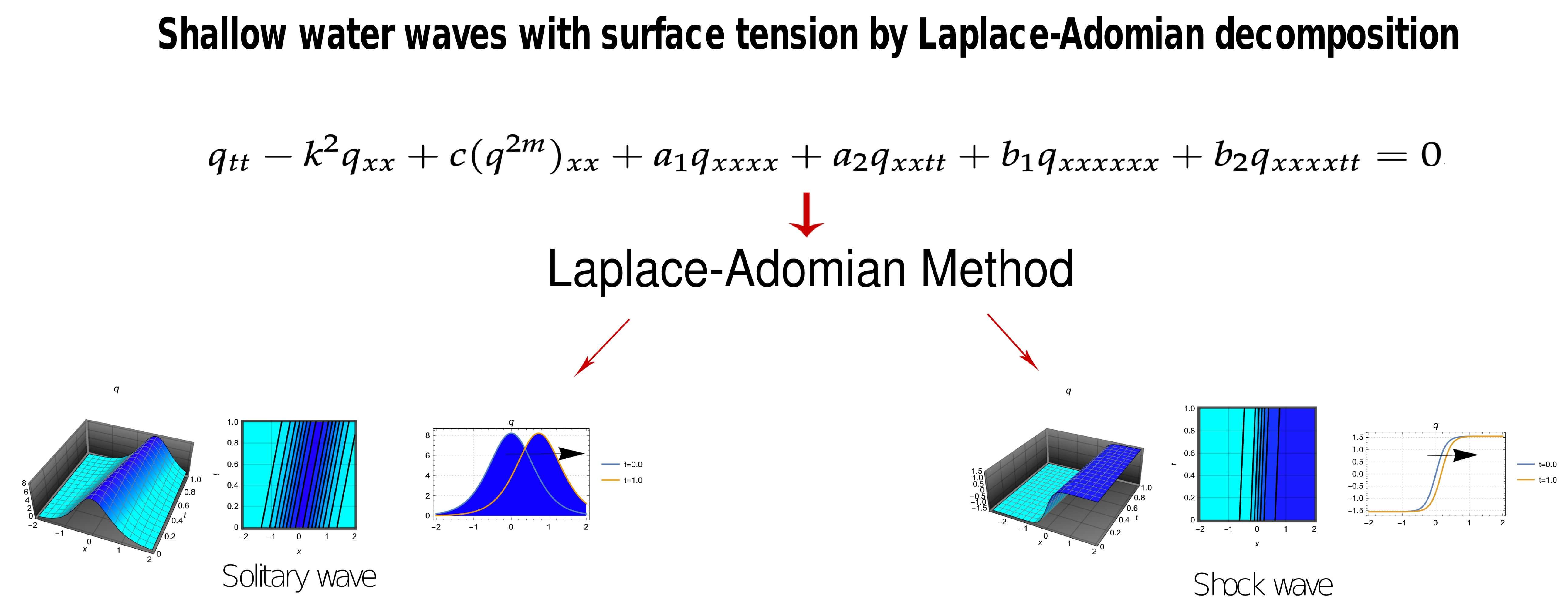
Shallow Water Waves with Surface Tension by Laplace–Adomian Decomposition
1 Applied Mathematics and Systems Department, Universidad Autónoma Metropolitana-Cuajimalpa, Vasco de Quiroga 4871, Mexico City, 05348, Mexico
2 Department of Computer Engineering, Biruni University, Istanbul, 34010, Turkey
3 Mathematics Research Center, Near East University, Nicosia, 99138, Cyprus
4 Faculty of Arts and Sciences, University of Kyrenia, Kyrenia, 99320, Cyprus
5 Faculty of Sciences and Environment, Department of Chemistry, Physics and Environment, Dunarea de Jos University of Galati, 47 Domneasca Street, Galati, 800008, Romania
6 Department of Physics, Sefako Makgatho Health Sciences University, Medunsa, Pretoria, 0204, South Africa
7 Department of Mathematics and Physics, Grambling State University, Grambling, LA 71245-2715, USA
8 Department of Physics and Electronics, Khazar University, Baku, AZ1096, Azerbaijan
9 Department of Applied Sciences, Cross-Border Faculty of Humanities, Economics and Engineering, Dunarea de Jos University of Galati, 111 Domneasca Street, Galati, 800201, Romania
10 Department of Mathematics and Applied Mathematics, Sefako Makgatho Health Sciences University, Medunsa, Pretoria, 0204, South Africa
* Corresponding Author: Anjan Biswas. Email:
(This article belongs to the Special Issue: Recent Advancements in Wave Dynamics Models for Fluids: Analytical and Numerical Approaches)
Fluid Dynamics & Materials Processing 2025, 21(9), 2273-2287. https://doi.org/10.32604/fdmp.2025.067959
Received 17 May 2025; Accepted 01 September 2025; Issue published 30 September 2025
 View Full Text
 Download PDF
Abstract
This study presents a numerical investigation of shallow water wave dynamics with particular emphasis on the role of surface tension. In the absence of surface tension, shallow water waves are primarily driven by gravity and are well described by the classical Boussinesq equation, which incorporates fourth-order dispersion. Under this framework, solitary and shock waves arise through the balance of nonlinearity and gravity-induced dispersion, producing waveforms whose propagation speed, amplitude, and width depend largely on depth and initial disturbance. The resulting dynamics are comparatively smoother, with solitary waves maintaining coherent structures and shock waves displaying gradual transitions. When surface tension is incorporated, however, the dynamics become significantly richer. Surface tension introduces additional sixth-order dispersive terms into the governing equation, extending the classical model to the sixth-order Boussinesq equation. This higher-order dispersion modifies the balance between nonlinearity and dispersion, leading to sharper solitary wave profiles, altered shock structures, and a stronger sensitivity of wave stability to parametric variations. Surface tension effects also change the scaling laws for wave amplitude and velocity, producing conditions where solitary waves can narrow while maintaining large amplitudes, or where shock fronts steepen more rapidly compared to the tension-free case. These differences highlight how capillary forces, though often neglected in macroscopic wave studies, play a fundamental role in shaping dynamics at smaller scales or in systems with strong fluid–interface interactions. The analysis in this work is carried out using the Laplace-Adomian Decomposition Method (LADM), chosen for its efficiency and accuracy in solving high-order nonlinear partial differential equations. The numerical scheme successfully recovers both solitary and shock wave solutions under the sixth-order model, with error analysis confirming remarkably low numerical deviations. These results underscore the robustness of the method while demonstrating the profound contrast between shallow water wave dynamics without and with surface tension.Graphic Abstract
Keywords
The theory of shallow water waves is a long-standing topic of interest in the fluid dynamics community ever since the solitary waves were discovered during a horse-drawn carriage in the canal of Edinburgh. Several mathematical models have been proposed, and they have all been analyzed over time. The first model that was extensively studied in this context is the Korteweg-de Vries (KdV) equation, which was followed by the modified KdV equation. Subsequently, many models, to address shallow water wave dynamics, emerged with time. They are the Boussinesq equation, Kawahara equation, Camassa-Holm equation and several others.
Shallow water wave dynamics, though traditionally rooted in geophysical and coastal engineering studies, hold significant relevance in materials science and fluid-structure interaction (FSI). These wave models capture essential features of dispersive and nonlinear wave propagation, making them valuable tools for understanding wave-induced stresses and responses in flexible or deformable structures. In materials science, such insights are crucial when evaluating the mechanical behavior of thin films, membranes, and soft composites subjected to dynamic fluid environments.
In the context of FSI, shallow water wave models help simulate the interaction between wave fronts and material surfaces, revealing critical information about fatigue, resonance, and structural deformation under transient loads. For instance, micro- and nano-scale materials used in sensors or biomedical devices may interact with fluid interfaces in ways that mirror shallow wave behavior, particularly when capillarity and surface tension play a role. Additionally, the incorporation of surface tension effects into shallow water wave equations enhances the applicability of these models to scenarios involving liquid–solid boundaries, such as in microfluidic channels or soft robotics.
The effects of surface tension have been incorporated into just a small number of the most recent models that were previously mentioned. This aspect was first taken up during 2002 and 2006 [1,2], respectively. This was for the Boussinesq equation. Later the model was extensively studied analytically with the effect of surface tension included. It must be noted that the surface tension effect leads to the inclusion of sixth-order dispersion that extends the familiar Boussinesq equation that comes with fourth-order dispersion. The solitary wave and shock wave solution to this sixth-order Boussinesq equation was recovered by the aid of undetermined coefficients during 2023 [3]. The conservation laws were also identified using the multipliers approach. Subsequently, the perturbed version of the sixth-order Boussinesq equation was addressed and its solitary waves and shock waves were retrieved and reported during 2025 [4].
Moving further along, after the analytical studies, it is now time to take a look at this model from a numerical perspective. The current paper does exactly that. This sixth-order Boussinesq equation is studied numerically in the current paper with the aid of the Laplace-Adomian decomposition method (LADM). This integration scheme is an extension of the pre-existing versions of the Adomian decomposition, namely the improved Adomian decomposition method. This improved version of the Adomian decomposition scheme was successfully implemented in a couple of models from Quantum Optics [5,6].
In the current paper, the LADM integration scheme retrieves solitary waves and shock waves. The error analysis of this scheme is also displayed, for solitary waves as well as shock waves, and the observation is that it is impressively low, of the order of 10−8. The details are chalked out in the rest of the paper after a quick revisitation of the model and a succinct recapitulation of the scheme.
2 The Model of the Sixth-Order Boussinesq Equation
The Boussinesq equation characterizing the motion of long waves traveling bidirectionally in shallow water under the influence of gravity is expressed as
A number of variants of Eqs. (1) and (2) have been examined in the literature. A generalization implies replacing the nonlinear term q2 with a nonlinear differential function f(q). A further generalization involved accounting for high dispersion components and incorporating surface tension effects. These generalizations result in the equation
The independent variables are the spatial variable x and the temporal variable t, whereas the dependent variable, representing the wave structure, is represented as q(x, t). The wave operator is represented by the first two terms, where k corresponds to the wave number. The parameter m is the general power law parameter, and the nonlinearity coefficient is denoted by c. This parameter provides the model with a generalized nature. In addition, the fourth-order dispersion parameters, which are caused by the effects of ai, are connected in the original model from the Navier–Stokes equation. On the other hand, the coefficients of bi come from the surface tension effect.
Eq. (3) is referred to as the Sixth-Order Boussinesq Equation (6BE) and was formulated based on the basic principles in the year 2006 in [1]. Later, during 2023, several analytical studies with the model have been conducted such as the retrieval of the analytical form of solitary and shock waves, recovery of the conservation laws and such [3]. The current paper addresses the study of shallow water waves, with the effect of surface tension included, numerically, for the first time.
SBE is used in various mathematical models for real-world situations, like studying vibrations in nonlinear atomic chains [10], solving some microstructure problems [11], and examining the movement of inviscid flow in shallow layers of fluid [2]. An interesting study on waves and solitons can be found at [12]. These applications highlight the versatility of the SBE, as it provides insights into complex phenomena across different scientific fields. Furthermore, ongoing research continues to explore its potential in new areas, enhancing our understanding of both theoretical and practical aspects of fluid dynamics.
Eq. (3) has been extensively studied, analyzed, and resolved using a variety of methodologies in the specific case of m = 1 [13,14,15,16,17,18]. The results suggest that the fundamental ideas are more profoundly understood as a consequence of the consistent behavior observed across various approaches. Additionally, these findings open the door to the investigation of complex scenarios in which m ≠ 1. In the current paper, we introduce a novel method for solving (3) when the parameter value is m ≠ 1. The proposed method is the Adomian decomposition method improved with the combination of the Laplace transform.
This section will illustrate the general form of both solitary waves and shock waves, which are solutions to the 6BE. The solution structure of such waves inherently generates the parametric constraints. The subsequent information is also listed and presented.
3.1 Solitary Wave Type Solutions
The authors in [3,4] have only recently found the solitary wave type solutions for Eq. (3) using the undetermined coefficients technique, which is expressed as
The amplitude A1 of the wave is
The velocity of the wave is given by
This demonstrates that the 6BE will have solitary waves as long as the two sixth-order dispersion terms have opposing signatures.
The inverse width B1 of the wave is
Consequently, the nonlinearity of the power law indicates the presence of solitary waves, provided that the constraint on m is supported.
The authors in [3,4] have only recently found the shock wave type solutions for Eq. (3) using the undetermined coefficients technique, which is expressed as
The amplitude A2 of the wave is
The velocity of the wave is given by
This confirms that the 6BE will have solitary waves as long as the two sixth-order dispersion terms have opposing signatures.
The inverse width B2 of the wave is
As a consequence, the nonlinearity of the power law suggests the existence of shock waves, provided that the constraint m = 3/2 is satisfied.
4 The Laplace-Adomian Decomposition Method
This section shows the general procedure for a numerical treatment of Eq. (3), which is based on the initial conditions provided for solitary waves and shock waves. The present scenario employs the Laplace–Adomian decomposition method (LADM), originally established by Refs. [19,20]. This method helps to break down complicated equations into simpler parts, making it easier to find accurate solutions for both solitary and shock wave situations.
Before establishing the steps of the method, we can write Eq. (3) as:
In addition, in (20), N symbolizes a nonlinear operator acting on q by
The following are the steps that are involved in the procedure of the method:
Step 1:
Apply the temporal Laplace transform
With the assumption that
The values of q(x, 0), qxx(x, 0), q4x(x, 0), etc., are calculated from the initial conditions associated with the waveforms listed in Section 3.
Step 2:
The function that is unknown q may be expressed as an infinite set of summands by using the typical Adomian decomposition method:
Furthermore, the nonlinear term N is expressed as an infinite series of Adomian polynomials in a single variable,
The Adomian polynomials Qn in a single variable may be derived for all types of nonlinearity, computed using the following formulae [21]:
These polynomials provide a systematic way to handle nonlinear terms in differential equations, enabling the construction of a series solution that converges to the desired function. By applying these polynomials, one can effectively separate the linear and nonlinear components, simplifying the analysis and solution of complex problems.
Substituting Eqs. (27) and (26) into Eq. (25) gives
Utilizing the linearity of the Laplace transform in Eq. (28) and equating both sides of the equation, we get the subsequent recursive formula:
Step 3:
We will consider the inverse Laplace transform
Similarly, applying the inverse Laplace transform in Eq. (29) to obtain:
Eqs. (31) and (32) allow us to determine each term of the function sequence
The solution derived from the suggested approach is expressed as an infinite series, represented by:
The deduced series solution may converge to an exact solution, required that such a solution exists. Alternatively, the series solution may be employed for numerical applications. For further information concerning the convergence of the suggested technique, consult Refs. [22,23].
As a result, a truncated series solution with N components is obtained as
The series solution (34) works well for numerical applications.
The subsequent section presents numerical examples to demonstrate the algorithm’s high accuracy and efficiency as offered by the suggested technique.
5 Numerical Simulation of Wave-Type Solutions
This section will simulate wave solutions for Eq. (3) utilizing the algorithm explained in Section 4. We will derive the initial conditions for each simulation from the general waveforms presented in Section 3. These initial conditions will provide the necessary parameters to accurately model the wave behavior as described in the equations. By referencing the general waveforms, we ensure that our simulations are grounded in established theoretical frameworks. The Mathematica 14.2.1 software is employed to generate the numerical simulation results.
5.1 Simulation of Solitary Wave Solutions and Graphical Representations
We will consider the three nonlinear cases in Table 1 when simulating solitary waves using LADM. It is crucial to keep in mind that m > 1/2 is one of the conditions for the existence of solitary waves in Section 3.1. This analysis is essential for validating the theoretical predictions and ensuring the reliability of the simulation results.
Table 1: Data for the simulation of solitary waves in 6BE that have different nonlinearities.
| Cases | Nonlinear Term | ||||||||
|---|---|---|---|---|---|---|---|---|---|
| 15 | |||||||||
| 15 | |||||||||
| 15 |
To implement the algorithm offered by LADM via Eqs. (31) and (32), we must take into account the general solitary waveforms illustrated in Section 3.1; that is, we must consider:
Moreover, using Formula (27), the first Adomian polynomials to decompose the nonlinear term q3/2 in the case m = 3/4 are given by:
These polynomials serve as the foundation for constructing a convergent series solution to the nonlinear problem at hand.
Also, using Formula (27), the first Adomian polynomials to decompose the nonlinear term q3 in the case m = 3/2 are given by:
Finally, the first Adomian polynomials to decompose the nonlinear term q5 in the case m = 5/2 are given by:
The graphical results of the solitary wave simulation using the algorithm developed by LADM are illustrated in Fig. 1, Fig. 2 and Fig. 3, which display the three cases enumerated in Table 1. The simulations illustrate the behavior of solitary waves in a selection of conditions, emphasizing the significant differences in propagation speed and amplitude. Additionally, we have included a comparison of the error generated by the Adomian decomposition method (ADM) in each figure. This method produces a slightly higher level of error than the LADM. The data used in the simulations conducted by the ADM is identical to that used in the LADM simulations. These visual representations offer valuable insights into the dynamics of wave actions and their implications for future research.
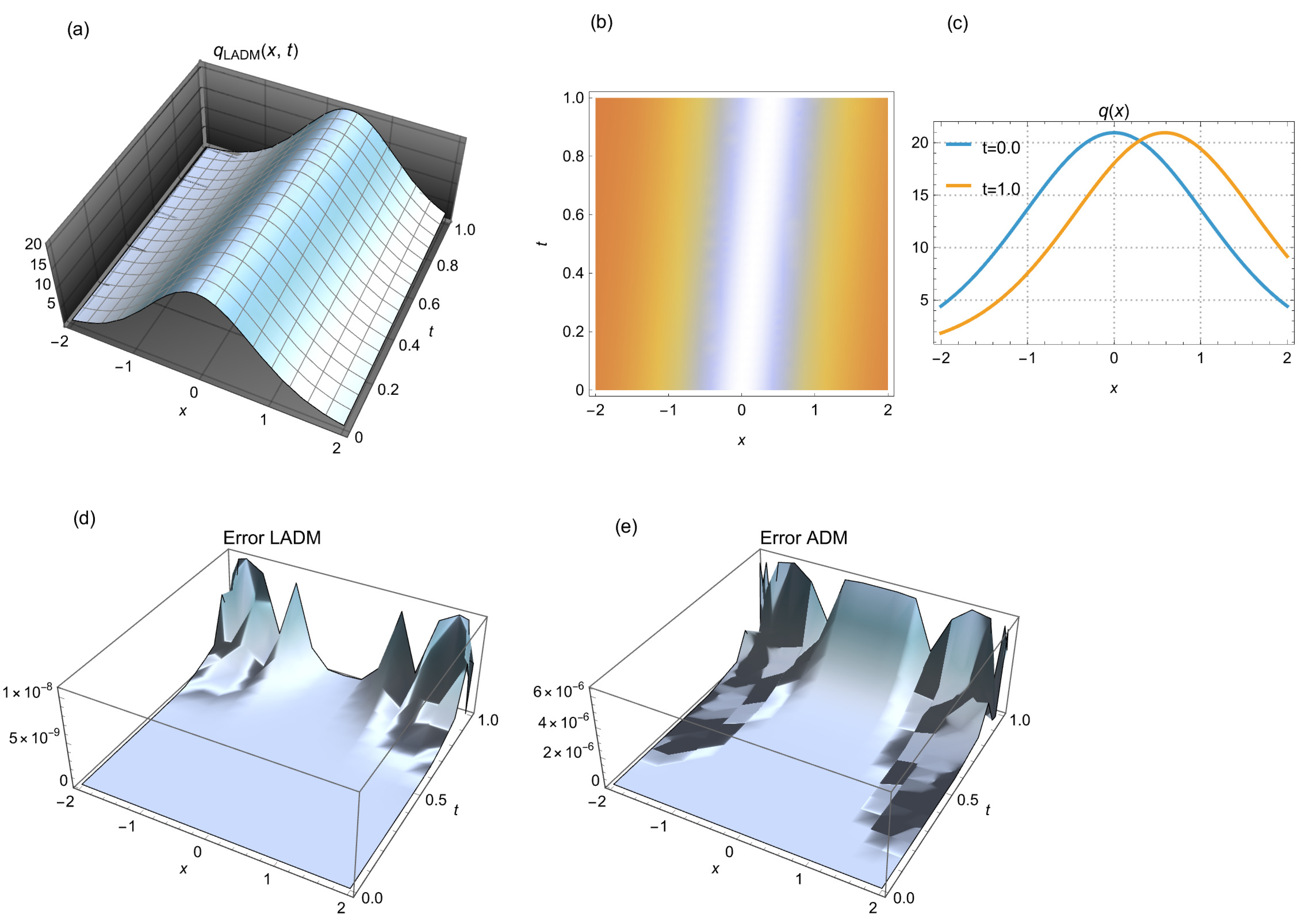
Figure 1: (a) 3D solitary wave simulated by LADM, (b) 2D density depiction of the corresponding wave, and (c) 2D time evolution for different time points. (d) error in the simulation by LADM, and (e) error in the simulation by ADM. We consider a scenario where m = 3/4 and N = 15 steps are used.
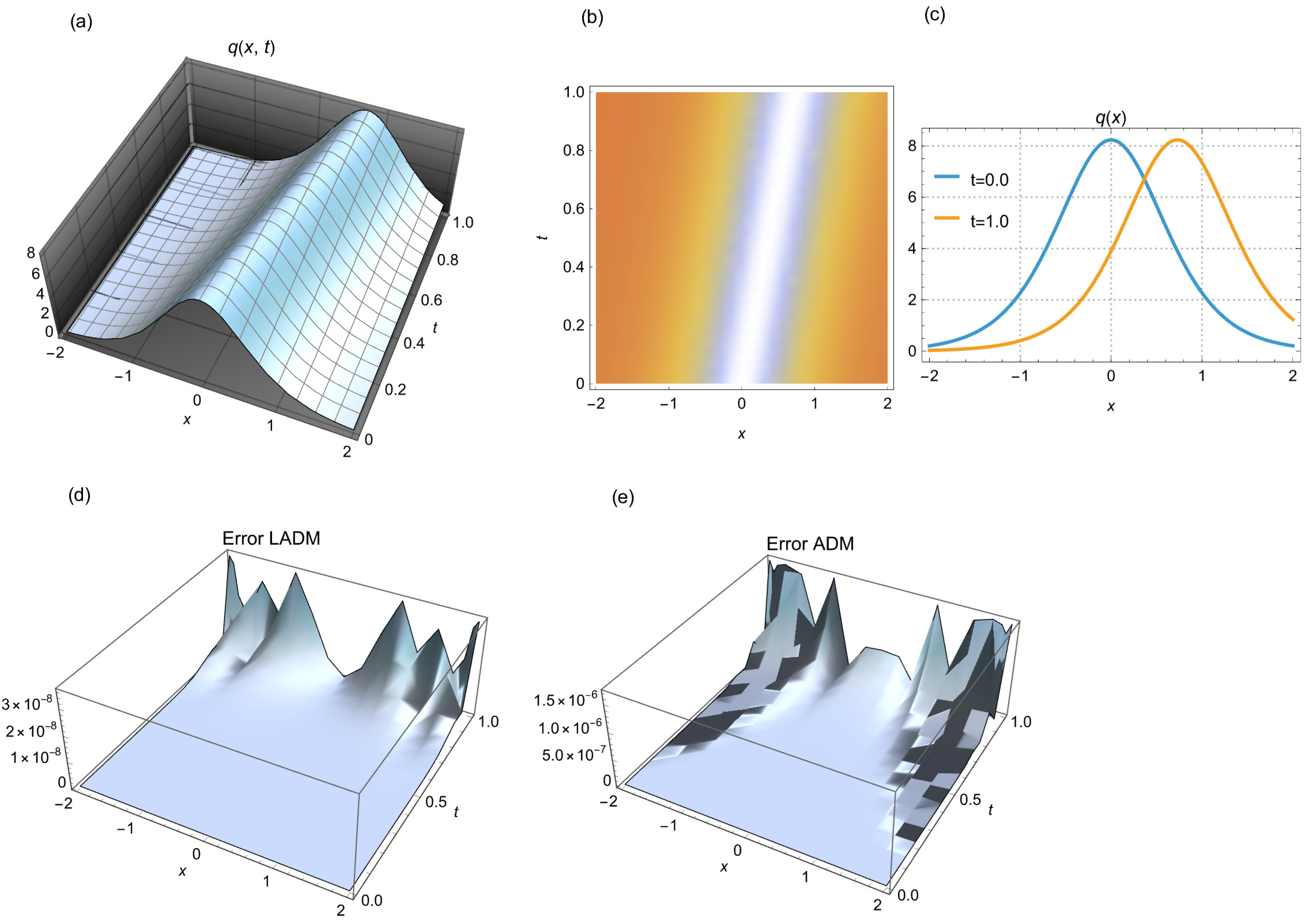
Figure 2: (a) 3D solitary wave simulated by LADM, (b) 2D density depiction of the corresponding wave, and (c) 2D time evolution for different time points. (d) error in the simulation by LADM, and (e) error in the simulation by ADM. We consider a scenario where m = 3/2 and N = 15 steps are used.
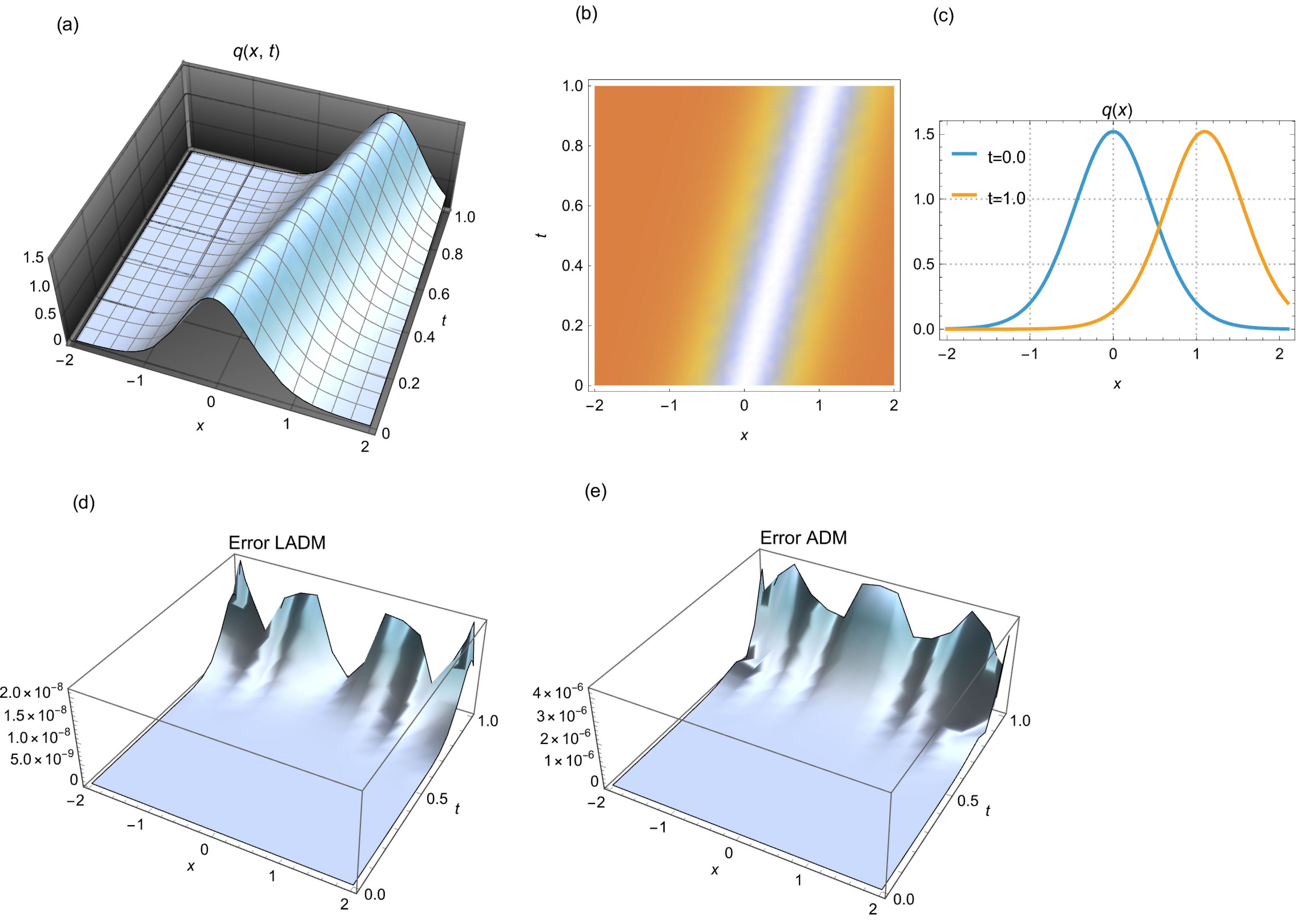
Figure 3: (a) 3D solitary wave simulated by LADM, (b) 2D density depiction of the corresponding wave, and (c) 2D time evolution for different time points. (d) error in the simulation by LADM, and (e) error in the simulation by ADM. We consider a scenario where m = 5/2 and N = 15 steps are used.
5.2 Simulation of Shock Wave Solutions and Graphical Representations
We will consider the three nonlinear cases in Table 2 when simulating shock waves using LADM. It is necessary to consider that the conditions established in Section 3.2 require the existence of shock waves for 6BE only if β = 1. Consequently, the sole supported nonlinearity is q3, which corresponds to m = 3/2. This analysis is essential for validating the theoretical predictions and ensuring the reliability of the simulation results.
Table 2: Data for the simulation of shock waves in 6BE.
| Cases | Nonlinear Term | ||||||||
| (i) | 15 | ||||||||
| (ii) | 15 | ||||||||
| (iii) | 15 |
Also, using Formula (27), the first Adomian polynomials to decompose the nonlinear term q3 in the case m = 3/2 are the same as those obtained in the second simulation example in Table 1.
The graphical results of the solitary wave simulation using the algorithm developed by LADM are illustrated in Fig. 4, Fig. 5 and Fig. 6, which display the three cases enumerated in Table 2. The simulations illustrate the behavior of solitary waves in a selection of conditions, emphasizing the significant differences in propagation speed and amplitude. Additionally, we have included a comparison of the error generated by the Adomian decomposition method (ADM) in each figure. This method produces a slightly higher level of error than the LADM. The data used in the simulations conducted by the ADM is identical to that used in the LADM simulations. These visualisations show wave action dynamics and its implications for future study.
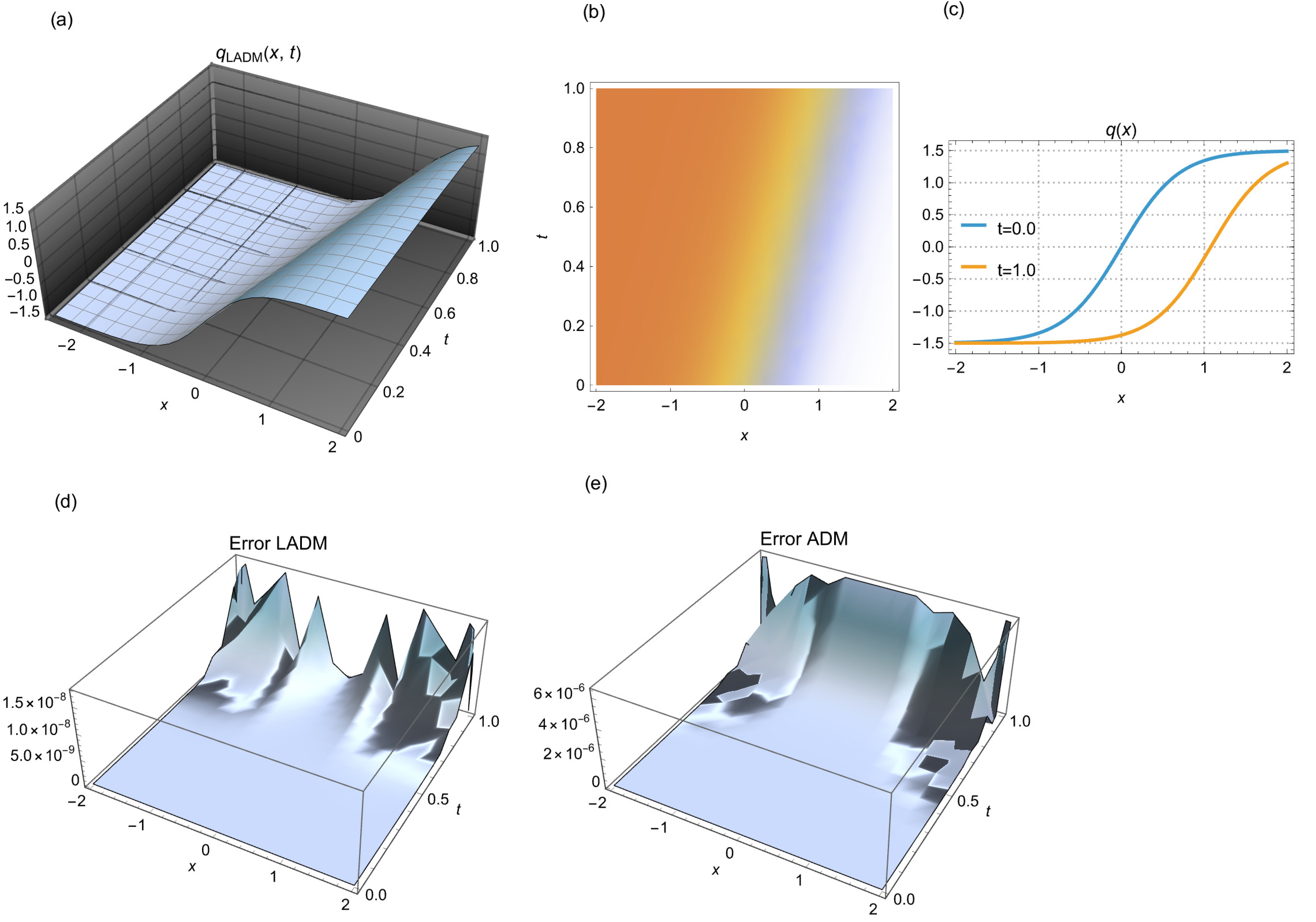
Figure 4: (a) 3D shock wave simulated by LADM, (b) 2D density depiction of the corresponding wave, and (c) 2D time evolution for different time points. (d) error in the simulation by LADM, and (e) error in the simulation by ADM. For the case (i) of Table 2 with N = 15 steps.
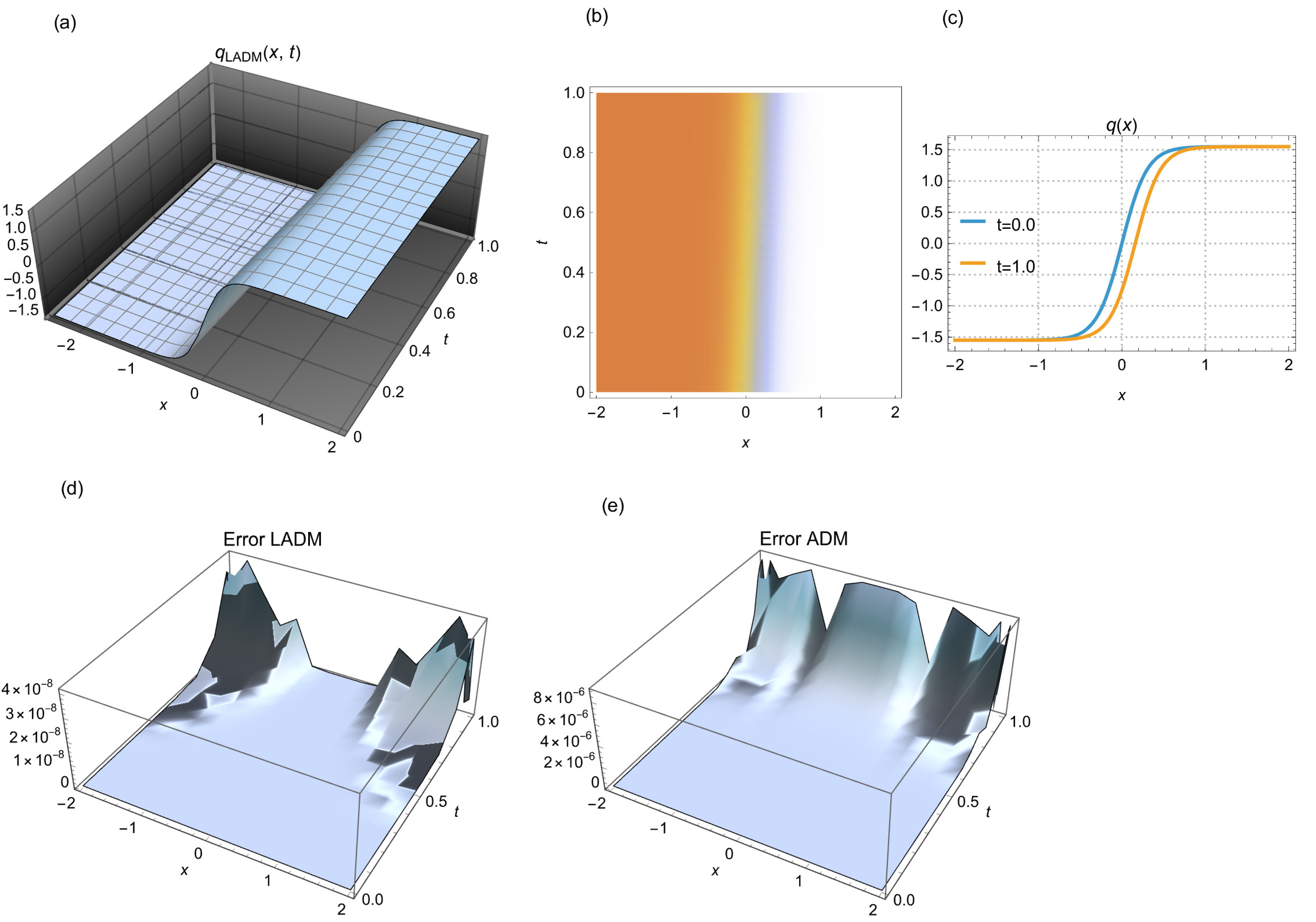
Figure 5: (a) 3D shock wave simulated by LADM, (b) 2D density depiction of the corresponding wave, and (c) 2D time evolution for different time points. (d) error in the simulation by LADM, and (e) error in the simulation by ADM. For the case (ii) of Table 2 with N = 15 steps.
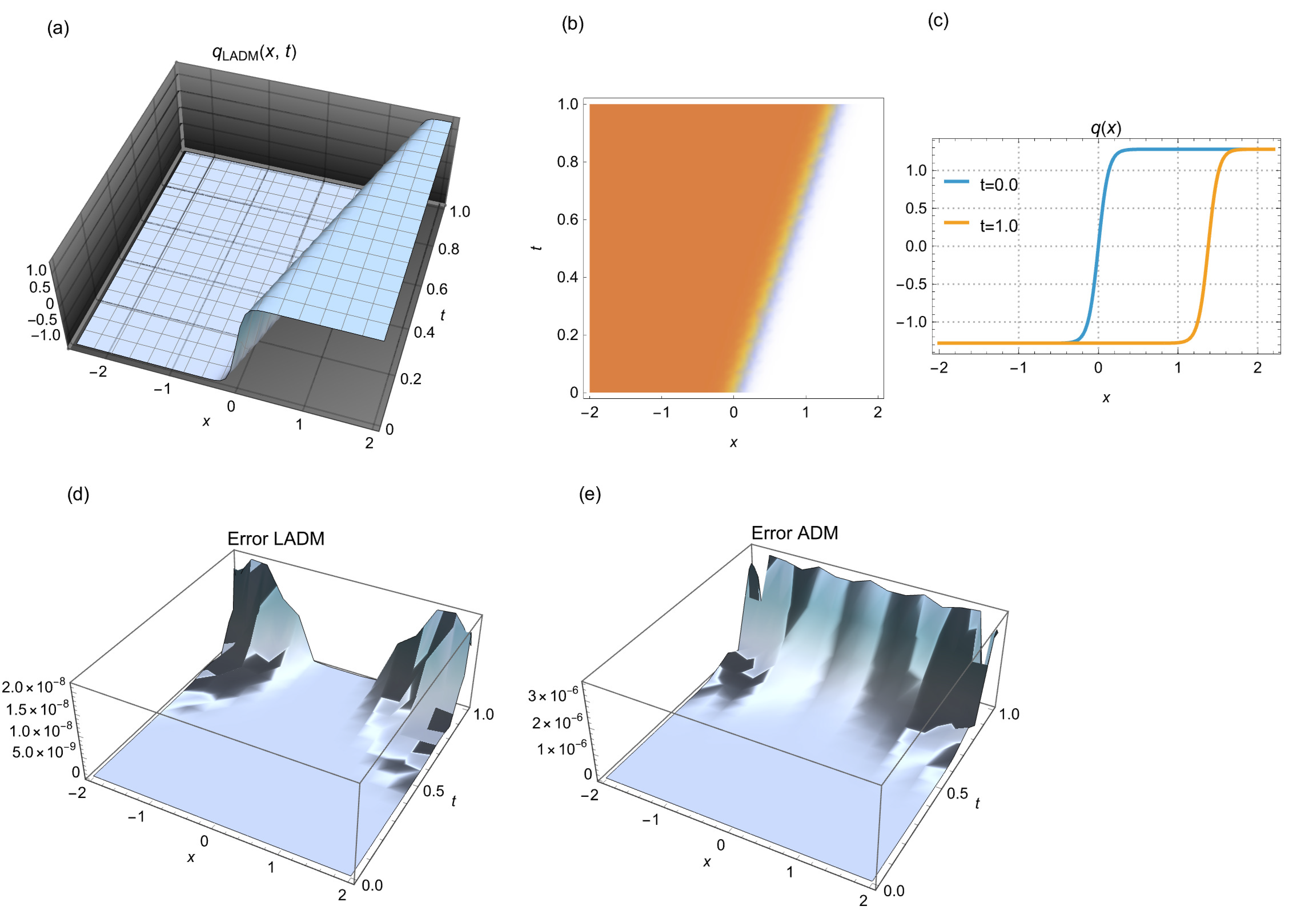
Figure 6: (a) 3D shock wave simulated by LADM, (b) 2D density depiction of the corresponding wave, and (c) 2D time evolution for different time points. (d) error in the simulation by LADM, and (e) error in the simulation by ADM. For the case (iii) of Table 2 with N = 15 steps.
The current paper retrieves solitary waves and shock waves that emerged from the sixth-order Boussinesq equation, which models shallow water wave dynamics in presence of surface tension. The Laplace-Adomian decomposition scheme has made this recovery possible with a stunningly low error measure. The solitary waves and shock wave solutions are numerically addressed using this integration algorithm. The sound results of the work pave the way for future research in this direction with the model.
Later, the shallow water wave dynamics with multi-layer fluids will be addressed. The corresponding vector coupled model of the sixth-order Boussinesq equation will be formulated and subsequently analyzed analytically as well as numerically. The results of such research activities will be disseminated over time.
Acknowledgement:
Funding Statement: The authors received no specific funding for this study.
Author Contributions: Oswaldo González-Gaxiola: Conceptualization, Methodology, Formal analysis, Writing—original draft; Yakup Yildirim: Project administration, Investigation; Luminita Moraru: Data Curation, Writing—review; Anjan Biswas: Conceptualization, Supervision, Project administration, Writing—review. All authors reviewed the results and approved the final version of the manuscript.
Availability of Data and Materials: The data that support the findings of this study are available from the corresponding author upon reasonable request.
Ethics Approval: Not applicable.
Conflicts of Interest: The authors declare no conflicts of interest to report regarding the present study.
References
1. Daripa P. Higher-order Boussinesq equations for two-way propagation of shallow water waves. Eur J Mech-B/Fluids. 2006;25(6):1008–21. doi:10.1016/j.euromechflu.2006.02.003. [Google Scholar] [CrossRef]
2. Daripa P, Dash RK. Weakly non-local solitary wave solutions of a singularly perturbed Boussinesq equation. Math Comput Simul. 2001;55:393–405. doi:10.1016/S0378-4754(00)00288-3. [Google Scholar] [CrossRef]
3. Biswas A, Vega-Guzman J, Bansal A, Kara AH, Aphane M, Yildirim Y, Alshehri HM. Solitary waves, shock waves and conservation laws with the surface tension effect in the Boussinesq equation. Proc Est Acad Sci. 2023;72(1):17–29. doi:10.3176/proc.2023.1.03. [Google Scholar] [CrossRef]
4. Kaur L, Yildirim Y, Adem AR, Moraru L, Biswas A. Perturbation of solitary waves and shock waves with surface tension. Contemp Math. 2025;6(2):1756–83. doi:10.37256/cm.6220256307. [Google Scholar] [CrossRef]
5. Al Qarni AA, Bodaqah AM, Mohammed ASHF, Alshaery AA, Bakodah HO, Biswas A. Dark and singular cubic-quartic optical solitons with Lakshmanan-Porsezian-Daniel equation by the improved Adomian decomposition scheme. Ukr J Phys Opt. 2023;24(1):46–61. doi:10.3116/16091833/24/1/46/2023. [Google Scholar] [CrossRef]
6. Almalki AM, Al Qarni AA, Bakodah HO, Alshaery AA, Arnous AH, Biswas A. Cubic-quartic optical solitons with polarization-mode dispersion by the improved Adomian decomposition scheme. MethodsX. 2025;14:103191. doi:10.1016/j.mex.2025.103191. [Google Scholar] [CrossRef]
7. Boussinesq MJ. The theory of waves and eddies propagating along a horizontal rectangular channel imparts roughly similar velocities to the liquid within the channel, from the surface to the bottom. J Math Pures. 1872;2:55–108. (In French) [Google Scholar]
8. Barostichi RF, Figueira RO, Himonas AA. Well-posedness of the “good” Boussinesq equation in analytic Gevrey spaces and time regularity. J Differ Eq. 2019;267:3181–98. doi:10.1016/j.jde.2019.04.001. [Google Scholar] [CrossRef]
9. Christov CI, Maugin G, Velarde M. Well-posed Boussinesq paradigm equation with purely spatial higher-order derivatives. Phys Rev E. 1996;54:3621–37. doi:10.1103/PhysRevE.54.3621. [Google Scholar] [CrossRef]
10. Feng B, Kawahara T, Mitsui T, Chan Y. Solitary wave propagation and interactions for a sixth-order generalized Boussinesq equation. Int J Math Math Sci. 2005;9:1435–48. doi:10.1155/IJMMS.2005.1435. [Google Scholar] [CrossRef]
11. Casasso A, Pastrone F, Samsonov A. Travelling waves in microstructure as exact solutions to the 6th order nonlinear equation. Acoust Phys. 2010;56(6):871–6. doi:10.1134/S1063771010060114. [Google Scholar] [CrossRef]
12. Li ZQ, Tian SF, Yang JJ. On the soliton resolution and the asymptotic stability of N-soliton solution for the Wadati-Konno-Ichikawa equation with finite density initial data in space-time solitonic regions. Adv Math. 2024;409:108639. doi:10.1016/j.aim.2022.108639. [Google Scholar] [CrossRef]
13. Yokus¸ A, Kaya D. Conservation laws and a new expansion method for sixth-order Boussinesq equation. AIP Conf Proc. 2015;1676:020062. doi:10.1063/1.4930488. [Google Scholar] [CrossRef]
14. Taskesen H, Polat N. Global existence for a double dispersive sixth-order Boussinesq equation. Contemp Anal Appl Math. 2013;1(1):60–9. [Google Scholar]
15. Recio E, Gandarias ML, Bruzon MS. Symmetries and conservation laws for a sixth-order Boussinesq equation. Chaos Solit Fractals. 2016;89:572–7. doi:10.1016/j.chaos.2016.03.029. [Google Scholar] [CrossRef]
16. Polat N, Pis¸kin E. Existence and asymptotic behavior of solution of Cauchy problem for the damped sixth-order Boussinesq equation. Acta Math Appl Sin. 2015;31(3):735–46. doi:10.1007/s10255-012-0174-2. [Google Scholar] [CrossRef]
17. Lai S, Wu Y. The asymptotic solution of the Cauchy problem for a generalized Boussinesq equation. Discrete Contin Dyn Syst Ser B. 2003;3(3):401–8. doi:10.3934/dcdsb.2003.3.401. [Google Scholar] [CrossRef]
18. Esfahani A, Muslu GM. Long time behavior of solutions to the generalized Boussinesq equation. Anal Math Phys. 2025;15:52. doi:10.1007/s13324-025-01048-8. [Google Scholar] [CrossRef]
19. Adomian G, Rach R. On the solution of nonlinear differential equations with convolution product nonlinearities. J Math Anal Appl. 1986;114(1):171–5. doi:10.1016/0022-247X(86)90074-0. [Google Scholar] [CrossRef]
20. Adomian G. Solving frontier problems of physics: the decomposition method. Boston, MA, USA: Kluwer Academic Publishers; 1994. doi:10.1007/978-94-015-8289-6. [Google Scholar] [CrossRef]
21. Duan JS. Convenient analytic recurrence algorithms for the Adomian polynomials. Appl Math Comput. 2011;217(13):6337–48. doi:10.1016/j.amc.2011.01.007. [Google Scholar] [CrossRef]
22. Hosseini MM, Nasabzadeh H. On the convergence of Adomian decomposition method. Appl Math Comput. 2006;182(1):536–43. doi:10.1016/j.amc.2006.04.015. [Google Scholar] [CrossRef]
23. González-Gaxiola O, Rach R, Ruiz de Chávez J. Solution for a rotational pendulum system by the Rach-Adomian-Meyers decomposition method. Nonlinear Eng. 2022;11(1):156–67. doi:10.1515/nleng-2022-0021. [Google Scholar] [CrossRef]
Cite This Article
 Copyright © 2025 The Author(s). Published by Tech Science Press.
This work is licensed under a Creative Commons Attribution 4.0 International License , which permits unrestricted use, distribution, and reproduction in any medium, provided the original work is properly cited.
 Downloads
 Citation Tools