
 Login
Login Register
 Submit a Paper
 Propose a Special lssue
 Open Access
ARTICLE

Dynamic Thermal Characteristics of Engine Oil Loop Integrated with Fuel Thermal Management
School of Aerospace Engineering, Tsinghua University, Beijing, China
* Corresponding Authors: Xianghua Xu. Email: ; Xingang Liang. Email:
(This article belongs to the Special Issue: Heat and Mass Transfer in Aero-Engines and Gas Turbines)
Frontiers in Heat and Mass Transfer 2026, 24(4), 1 https://doi.org/10.32604/fhmt.2026.084170
Received 17 April 2026; Accepted 12 June 2026; Issue published 31 August 2026
 View Full Text
 Download PDF
Abstract
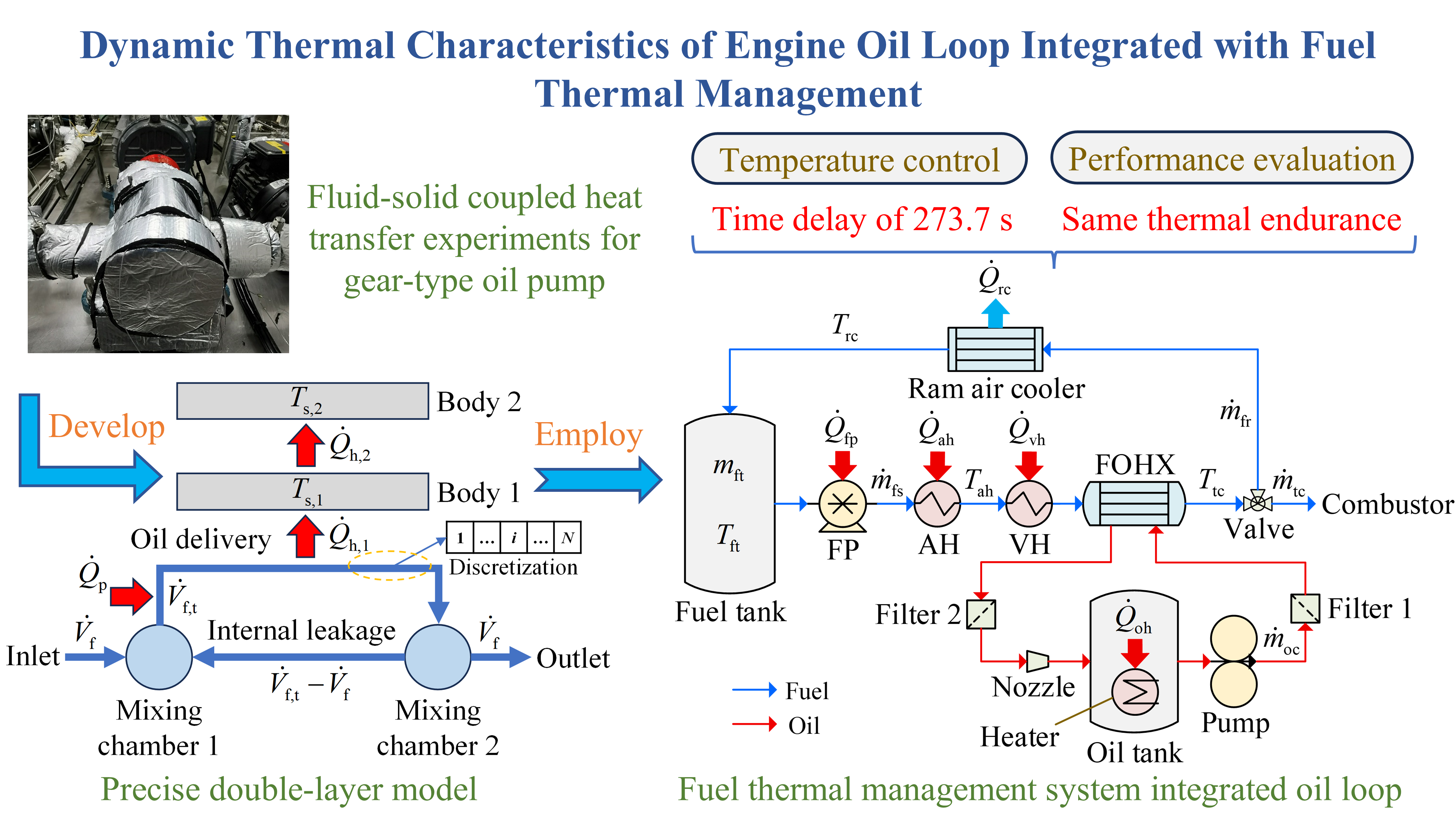
The rapid increase in onboard heat loads has made aircraft thermal management a critical issue. As an important part of the fuel thermal management system (FTMS), the dynamic thermal characteristics of the engine oil system (EOS) directly determine temperature regulation and fuel heat sink utilization, necessitating further investigation. In this paper, a novel dynamic heat transfer model for the oil pump was firstly developed through temperature step experiments. Subsequently, a transient flow and heat transfer model of the oil loop was established using the thermal fluid network (TFN) method, and the influence of thermal inertia on thermal response was analyzed. Finally, the impact of the dynamic thermal effects of the EOS on thermal management performance was quantitatively evaluated under an integrated FTMS architecture. Experimental results show significant temperature stratification within the pump body due to large heat conduction resistance. Compared with the single-layer model, the developed double-layer model achieves a 90.25% reduction in temperature prediction errors. In addition, increases in rotational speed and fluid temperature enhance the fluid-solid coupled heat transfer within the pump, while the increase in volumetric efficiency weakens this process. The relative error of the developed empirical correlation for heat transfer within the pump is less than 12%. During operating condition switching, the response delay in thermal parameters can reach 273.7 s, indicating that the fuel supply from the plane needs to be regulated in real time according to the varying oil heat load to prevent both system overtemperature or the waste of fuel heat sink, since the traditional quasi-steady regulation strategy leads to a temperature deviation of up to 4.37 K. Nevertheless, the total heat capacity within the EOS alternately stores and releases heat under a periodic combat mission, with the opposing effects on fuel heat sink consumption canceling each other out. In this case, the integrated FTMS achieves almost the same thermal endurance as that without considering the dynamic thermal effects of the oil loop. Therefore, the thermal inertia of the EOS must be considered in precise temperature control but can be neglected in thermal endurance evaluation. The findings of this paper provide strong support for dynamic thermal modeling of the EOS, system temperature control, and performance evaluation integrated with fuel thermal management.Graphic Abstract
Keywords
In recent years, aircraft performance has been continuously enhanced to accommodate increasingly complex flight missions, leading to a substantial rise in onboard heat loads and posing severe challenges for thermal management [1]. Additionally, heat rejection to ambient air is impeded by several factors: the extensive use of low-thermal-conductivity composites in the fuselage, stealth-imposed restrictions on air intake, and significant aerodynamic heating at high speeds [2–4]. To address this issue, fuel has emerged as the primary heat sink in advanced aircraft due to its large capacity and superior thermal stability [5], driving the rapid development of fuel thermal management system (FTMS) [6–10].
In the FTMS, fuel drawn from the fuel tank sequentially absorbs heat loads from airborne subsystems and the engine before entering the combustor. To meet cooling requirements and prevent fuel coking, multiple temperature limit points are typically set within the FTMS [11]. When the cooling fuel flow exceeds that required for combustion, the excess fuel, referred to as hot fuel return (HFR), is cooled by ram air and returned to the fuel tank. Under the combined effects of HFR and high airborne heat loads, the temperature of fuel entering the engine progressively increases, threatening the effectiveness of engine cooling [12,13]. Moreover, as the engine is positioned at the hottest end of the FTMS, its waste heat transferred to the fuel directly determines the aircraft’s thermal safety. Therefore, the thermal characteristics of engine thermal management subsystems require focused attention. Among engine heat loads, the heat load from the engine oil system (EOS) is inherent [14], which serves as the research focus of this paper.
Advanced EOS adopts a circulating loop design, with the oil tank typically kept in a hot state to facilitate gas removal [15]. Oil from the oil tank is cooled by fuel or air through heat exchangers before being supplied to the bearing chambers and gearboxes for lubrication and cooling, and then returns to the oil tank [16]. Similarly, there exists an upper limit on the operating temperature of oil due to oxidation stability [17], and enhancing the heat transfer capability of both heat exchangers [18,19] and circuits [20,21] is an essential approach to preventing oil thermal failure, which reduces the temperature difference for heat transfer. In addition, the heat transfer rate from the EOS to the fuel, referred to as oil heat load within the FTMS, directly affects both fuel flow regulation and fuel heat sink consumption [7], and thus needs to be accurately captured rather than assumed as fixed values. In steady-state studies, Lu et al. [22] developed simulation software for the EOS based on the thermal fluid network (TFN) method to obtain the distribution of flow and heat transfer parameters. Liu et al. [23] established a simulation model of the EOS with multiple circuits using the heat current method and elucidated the variations of fluid temperatures and heat transfer rates with boundary parameters. Leng et al. [24] calculated bearing heat generation and system heat dissipation under various operating conditions based on an airframe-engine integration approach. Nevertheless, rapid variations in oil heat generation frequently occur during flight due to its direct correlation with engine thrust and rotational speed [15], while the cooling fuel flow is continuously regulated under temperature limitations [7], highlighting the thermal response delay caused by the fluid and solid heat capacities of components within the system. Gou et al. [25] reported the significant effect of fluid-solid coupled heat transfer on the fuel temperature at the fuel nozzle. Consequently, establishing a dynamic heat transfer model of the EOS is crucial for accurately predicting the oil heat load.
From a component perspective, research on dynamic heat transfer models for tubes has been relatively thorough. Han [26] established a one-dimensional transient flow and heat transfer model for tubes applicable to TFN calculations through element discretization. Lin et al. [27] further considered the influence of additional heat capacity caused by supports and other structures. In contrast, research on dynamic heat transfer models for pumps with large solid heat capacity remains in the exploratory phase. Computational fluid dynamics (CFD) is a commonly used approach for obtaining transient flow and heat transfer parameters in pumps. Zhai et al. [28] proposed a stepwise method based on different time scales for simulating fluid-solid coupled heat transfer in hydrogen circulating pumps (HCP), implemented with the STAR-CCM software. Li et al. [29] revealed the dynamic evolution of key parameters within an aviation piston pump using the ANSYS software. Cui and Shi [30] employed the Pumplinx software to calculate the transient thermal effects of the flow field within an internal gear pump. However, CFD suffers from low computational efficiency, which hinders its integration into fast-response system-level dynamic simulations. To accelerate calculations, Yang et al. [31] developed a machine learning model for an external gear pump based on experimental data. Additionally, some scholars adopted the lumped parameter method (LPM) to divide control volumes inside the pump, thereby quantitatively evaluating the fluid-solid coupled heat transfer processes [32–34]. Nevertheless, the aforementioned models either rely on extensive experimental data or require detailed structural parameters and complex empirical heat transfer correlations, resulting in limited applicability and necessitating further improvement.
Research on the overall dynamic thermal characteristics of the EOS remains scarce. Wang et al. [14] investigated the dynamic thermal behavior of the EOS across the mission profile based on the AMESim software, providing support for the reuse of oil waste heat in the environmental control system (ECS). Yang et al. [35] analyzed the dynamic thermal performance of a fuel-oil thermal management system using the TFN method and achieved effective regulation of limit temperatures through a variable-step control algorithm, in which only a transient flow and heat transfer model for tubes was established, without accounting for the dynamic thermal effects of the oil pump or quantitatively evaluating the fluid-solid coupled heat transfer process. Yevlakhov et al. [36] calculated the dynamic temperature response of both fuel and oil under mode switching with the TFN method and discussed scenarios involving overtemperature. However, these studies lack a detailed discussion on the coupled effects of fluid and solid heat capacities on the system’s dynamic thermal characteristics, and the impact of thermal inertia within the EOS on fuel thermal management performance remains unclear.
In summary, to further investigate the dynamic thermal characteristics of the EOS integrated with fuel thermal management, the main contributions of this paper are as follows:
• An efficient transient flow and heat transfer model for the oil pump was constructed based on temperature step experiments, with the influence of operating parameters on fluid-solid coupled heat transfer mastered and the corresponding empirical correlation developed.
• A dynamic simulation model of the EOS was established using the TFN method, and the system’s thermal inertia was quantitatively evaluated.
• In the context of fuel thermal management, the impact of the dynamic thermal effects of the EOS on fuel flow regulation and fuel heat sink consumption in the FTMS was elucidated.
2 Dynamic Heat Transfer Model of Oil Pump
The experimental system for the transient flow and heat transfer characteristics of the oil pump is depicted in Fig. 1, where the pump is selected as an external gear pump (positive displacement type) commonly used in the EOS [15], and the working fluid is 4050 aviation lubricating oil [37]. The supply section comprises a cold oil tank and a hot oil tank, each equipped with a mixer to ensure uniform temperature distribution. Pumps 1 and 2 provide inlet pressurization for the oil pump to prevent cavitation. Pressure regulating valves 1 and 2 (PRV 1 and PRV 2) are employed to maintain the oil supply pressure, with excess oil bypassed to the supply tanks. Switching valve (SV) is a three-way valve that generates step changes in the oil pump’s inlet temperature to facilitate the observation of dynamic thermal characteristics. Needle valve (NV) is used to alter the volumetric efficiency of the oil pump by regulating its outlet pressure. All pumps are driven by variable-frequency motors, with their rotational speeds adjusted to meet the required oil flow rates. In this study, all experimental conditions adopt step changes from low to high temperatures. After the experiment, the used oil in the recycling oil tank returns to the supply tanks under the action of a cooler and a heater.

Figure 1: Schematic diagram of the experimental system’s working principle.
Sheathed T-type thermocouples T1 and T2 are installed upstream and downstream of the oil pump to measure fluid temperatures, respectively, and a surface-mounted T-type thermocouple cluster T3 is arranged on the external surface of the pump body to measure solid temperatures. Pressure taps P1 and P2 are positioned to obtain the pump’s pressure rise by a differential pressure gauge, and a gear flowmeter is placed downstream to measure the volumetric flow rate. All thermal-hydraulic data are recorded in real time at a time interval of 0.1 s. Fig. 2 exhibits the distribution of the oil pump’s temperature measurement points in detail, where T1 and T2 are installed at points a and b, respectively, and thermocouples 1–10 (T3) are distributed at different thickness positions of the pump body to measure temperature variations within the solid, including the end cover, side wall, shaft housing, and base. Specifically, temperature measurement points 3–6 are located at the thin-walled section, while other measurement points are located at the thick-walled section. To eliminate the effects of heat dissipation to the environment, the oil pump and its associated pipelines are fully covered with insulation layers. The performance parameters of the aforementioned sensors are listed in Table 1.

Figure 2: Distribution of temperature measurement points for the oil pump.

The oil pipelines within the experimental system are constructed from 316 L stainless steel circular tubes with inner and outer diameters of 8 and 10 mm, respectively. Due to installation requirements, T1 and T2 are positioned 5 cm away from the actual inlet and outlet of the oil pump, respectively. The transient flow and heat transfer model for tubes established in Ref. [26] is used to correct the temperature response delay caused by the connecting tubes, where the fluid-solid coupled heat transfer coefficients (HTC) under laminar and turbulent flows are calculated using the Sieder-Tate and Gnielinski correlations, respectively [38,39], and the Darcy friction factor for turbulent flow is determined by the Konakov formula [40]. The internal flows of an external gear pump are illustrated in Fig. 3. As the gear pair rotates, oil is delivered from the inlet to the outlet, with the motor speed regulated by a frequency converter. There exist two mixing chambers with the same volumes at the two ports, and a portion of the oil leaks from mixing chamber 2 to mixing chamber 1 under the action of differential pressure and gear engagement [41]. The incoming flow and internal leakage mix with the fluid in chamber 1 before entering the oil delivery path, and the two delivered oil streams mix with the fluid in chamber 2 before being discharged or leaking back to chamber 1. The oil pump is made of 304 stainless steel, with main parameters presented in Table 2, where

Figure 3: Schematic diagram of internal flows for an external gear pump.

2.2 Fluid-Solid Coupled Heat Transfer Modeling
When oil flows through the pump, the temperature response at the outlet is influenced not only by the fluid’s heat capacity within the pump but also by the heat transfer between the fluid and solid due to temperature difference, and the latter mechanism is the focus of this section. Unlike complex partitioning strategies for quantitative calculations [32–34], the solid zone, including the end cover, shell, gears, etc., is integrated here using the LPM, which reduces the number of heat transfer variables and facilitates the determination of unknown parameters from experimental data. Note that this modeling method is applicable to various types of pumps, demonstrating good generalizability. Additionally, inspired by the additional heat capacity method developed in Ref. [27], a layered model is further proposed to address the potential non-uniform temperature distribution within the solid zone caused by the thick pump body, in which the body is divided into two layers. The architectures of the two fluid-solid coupled heat transfer models are depicted in Fig. 4.

Figure 4: Fluid-solid coupled heat transfer models of gear pump based on the LPM. (a) Architecture of the single-layer model; (b) Architecture of the double-layer model.
Fig. 4a shows a single-layer model, characterized by treating the entire pump body as a single lumped element. Fig. 4b presents a double-layer model that divides the body into inner and outer layers (body 1 and body 2) to consider the temperature gradient within the body. In addition to the convective heat transfer between the fluid and solid in the single-layer model, the double-layer model also accounts for the heat conduction between the inner and outer layers. Next, governing equations for transient flow and heat transfer within the pump are established in detail. As the fluid is liquid, it is regarded as incompressible, with the average fluid temperature within the pump taken as its reference temperature. Besides, the temperatures of each body element are treated as their respective reference temperatures.
At the mixing chambers, conservations of mass and energy are satisfied:
where
To accurately capture the temperature response delay due to fluid transport from chamber 1 to chamber 2, the oil delivery path is discretized along the flow direction. Additionally, both heat generation and various fluid-solid coupled heat transfer processes within the fluid zone are uniformly incorporated into the delivery path to simplify modeling, yielding the following transient temperature equations for the fluid and solid elements in the two models [42]:
(a) Single-layer
(b) Double-layer
where
In Eqs. (3) and (5),
where
The volumetric efficiency of the pump (
Due to the difficulty in determining the heat transfer area (
where
To facilitate subsequent discussion, the mass fraction of the inner layer in the pump body (
During temperature step changes, the factors affecting the fluid-solid coupled heat transfer process include the flow distribution inside the pump and the thermophysical properties of both the fluid and the solid. The former is determined by

During the temperature step change, the unknown parameters
where M is the total number of recorded points during the step process.

Figure 5: Flowchart for inverting unknown parameters based on PSO method.
After calculation, the inversion results of the unknown parameters for the two models under the baseline condition are presented in Table 4, where the thermophysical properties of the fluid and solid are sourced from Refs. [37,44]. Since Eq. (15) represents the average error over thousands of measurement points, measurement uncertainty may induce a certain influence on the inversion results, which needs to be quantitatively evaluated. Here, random errors are added to the experimental results under the baseline condition according to the accuracy ranges of the sensors, and the unknown parameters of both the single-layer and double-layer models are inverted again. The calculation results show that after adding random errors,

The dynamic thermal comparisons of the two models are illustrated in Fig. 6, where

Figure 6: Dynamic thermal comparison results of the two models under the baseline condition. (a) Fluid temperatures of the single-layer model; (b) Solid temperatures of the single-layer model; (c) Fluid temperatures of the double-layer model; (d) Solid temperatures of the double-layer model; (e) Heat transfer rates of the two models.
Fig. 6a,c reveals that
In contrast, the double-layer model effectively addresses this issue, as shown in Fig. 6d, thereby achieving high-precision prediction of
It can be observed from Fig. 6d that
From the above analysis, it can be seen that the fluid-solid coupled heat transfer within the oil pump significantly influences the response of the outlet fluid temperature during the step-change process, which poses difficulties for system temperature control. To mitigate this phenomenon, two approaches can be adopted: reducing the intensity of the fluid-solid coupled heat transfer and lowering the heat storage capacity of the pump body. Specifically, the former can be achieved by reducing the fluid-solid coupled heat transfer area or by introducing thermal insulation materials with low heat conductivity into the pump body. The latter can be achieved by using high-strength materials to make the pump body thinner while still satisfying the mechanical performance requirements.
2.3 Analysis of Parameter Influence
A double-layer model for calculating the dynamic heat transfer process of the oil pump has been established in Section 2.2. Next, the influence of the oil pump’s operating parameters on


Figure 7: Variations of
Fig. 7a indicates that

Firstly,
Meanwhile, the flow Reynolds number of oil delivery path (
where
Based on parameter independence analysis,
where
Fig. 8 illustrates the fitting accuracy of Eq. (20), demonstrating that all experimental data points fall within a relative error brand of ±12%. This correlation provides a foundation for subsequent transient flow and heat transfer calculations of the EOS. Note that the form of Eq. (20) possesses a certain universality. By fitting the coefficients over a wider experimental range, the coverage of the entire flight mission profile can be achieved.

Figure 8: Statistical graph of calculation errors for the correlation.
3 Dynamic Thermal Characteristics of Oil Loop
In this subsection, a dynamic heat transfer model of the EOS embedded with the pump’s double-layer model is established. A typical architecture of the oil loop integrated with fuel thermal management is depicted in Fig. 9 [15], where the pump provides driving force for oil circulation (

Figure 9: Typical architecture of the EOS integrated with fuel thermal management.
Subsequently, the transient flow and heat transfer equations for the EOS are formulated. The flow in the system is treated as quasi-steady, as the fluid is incompressible [26]. Likewise, the pump is an external gear pump, with its oil delivery capability described as [41]:
where
The flow resistance within the tube is calculated by [46]:
where
The flow characteristics of local resistance components (filters and the nozzle) are uniformly given by [46]:
where
The FOHX is configured as a shell and tube type, with the fuel and oil flowing through the tube and shell sides, respectively. The tube bundle within the heat exchanger is arranged in a triangular pattern, and the baffle cut ratio is 25%. The flow resistance on the tube side is also calculated using Eq. (22), while the pressure drop on the shell side is determined by the Kern method [47]:
where
As for transient temperature calculations, the oil pump and tubes adopt the previously developed double-layer model and the discretization model from Ref. [26], respectively. Note that Eq. (20) is assumed to remain applicable for describing the fluid-solid coupled heat transfer within the pump during system-level simulation, even when the operating conditions fall outside its fitting range. On the one hand, the accuracy of this extrapolation can be guaranteed by the monotonic and smooth trends of
where
As the heat exchange interface between the oil loop and the fuel flow path, the dynamic thermal characteristics of the FOHX also influence the response of system thermal parameters to some extent. Nevertheless, this paper mainly focuses on the dynamic heat transport process from the oil-side outlet to the inlet of the FOHX within the oil loop, which provides a dynamic heat load boundary for the FTMS with quasi-steady models [6]. Moreover, considering the application of compact heat exchangers in advanced engines, the thermal inertia caused by the fluid and solid heat capacities within the FOHX is relatively small. Therefore, a quasi-steady assumption is temporarily adopted here to facilitate the temperature regulation of the fuel system. In our future work, the dynamic thermal model of the FOHX will be refined, and the corresponding fuel thermal management strategy will be further developed to execute high-precision control. Consequently, the heat transfer rate from the oil to the fuel (
where
The oil temperature within the oil tank (
where
Based on the above governing equations, the TFN method with series simplification is employed to solve the transient flow and heat transfer process of the oil loop [35,51]. Additionally, the energy analysis method from Ref. [7] is adopted for dynamic thermal calculations of the fuel flow path. To validate the accuracy of the dynamic simulation of the EOS, a comparison of transient flow and heat transfer parameters for the oil section is performed by increasing the HFR flow rate on the experimental setup from Ref. [45], as illustrated in Fig. 10, where the subscript “outl” denotes the outlet of the component. It can be inferred that the dynamic TFN method developed in this paper accurately captures the transient flow and heat transfer characteristics of the EOS.

Figure 10: Comparison of transient flow and heat transfer parameters for the EOS under HFR regulation. (a) Mass flow rate of the oil pump; (b) Outlet pressure of the oil pump; (c) Outlet temperature of the oil pump.
During the subsequent calculations, the lubricating oil and the solid materials of the oil pump and tubes are the same as those in Section 2, with the FOHX made of 316L stainless steel. Besides, the fuel is JP-8 aviation kerosene, and its thermophysical properties are taken from Ref. [52]. To ensure thermal safety, the upper temperature limits of the fuel (

3.2 Analysis of Thermal Inertia
Firstly, the influence of thermal inertia of the EOS on the response of system thermal parameters is discussed based on the transient flow and heat transfer model developed in Section 3.1. A step change in


Figure 11: Dynamic response of system thermal parameters under the step condition. (a) Limiting temperatures; (b) Heat storage rate of the oil tank; (c) Heat storage rates in the pipeline; (d) Heat transfer rate of the FOHX.
Fig. 11a shows that the EOS stays at a thermal steady state before point B, while a significant temperature response delay (from point B to point C) is observed at the monitoring points. After calculation, the effect duration of thermal inertia (

Figure 12: Comparison of dynamic thermal response with different
Fig. 12a shows that the monitoring temperatures rise faster after the step of
Fig. 11d illustrates the effect of thermal inertia on
Now, the key drawbacks of neglecting the thermal response delay of the oil loop in the regulation of the FTMS are displayed through two typical cases. Consider a scenario that

Figure 13: Variations of thermal regulation parameters in the two cases. (a) Combustion fuel temperature in case 1; (b) Fuel supply flow in case 1; (c) Combustion fuel temperature in case 2; (d) Fuel supply flow in case 2.
Fig. 13b,d shows the sudden changes of
From the above analysis, it can be concluded that the fluid and solid heat capacities introduce significant response delays and nonlinear characteristics in the thermal parameters of an integrated FTMS. In practical engineering applications, advanced controllers are required to address this issue. In recent years, linear quadratic regulator (LQR) [6] and model predictive control (MPC) [10,53] have been applied to the dynamic control of thermal and energy management systems. Based on their respective algorithm frameworks, LQR is more suitable for quasi-steady state linear control, while MPC can effectively handle nonlinear problems with time delays. Given that future complex flight missions would lead to more frequent variations in system heat loads, fuel supply, and oil supply, along with an increasing number of control parameters and constraints, MPC, with stronger capability in nonlinear optimization and better adaptability, holds greater potential. In addition, He et al. [54] developed a constrained MPC controller based on heat current models, providing theoretical support for future dynamic high-precision optimal control of the integrated FTMS with multiple constraints.
3.3 Evaluation of Thermal Management Performance
In this subsection, the influence of thermal inertia of the oil loop on the fuel thermal management performance of the FTMS is evaluated using a typical architecture of the integrated fuel-oil system, as shown in Fig. 14.

Figure 14: Typical architecture of the FTMS integrated with a dynamic oil loop.
Fuel from the fuel tank is initially extracted by a fuel pump (FP), and it then sequentially flows through the airborne heater (AH), viscous dissipation heater (VH), and the FOHX, before being supplied to the combustor, where the first two heat loads are denoted as

The FTMS is calculated based on the simulation method in Ref. [7], where
where the subscript “fp” represents the FP,
The main component parameters of the FTMS adopted in this paper are listed in Table 10 [6,7], where

In this paper, thermal endurance (
where
Therefore,

Figure 15: Flowchart of FTMS simulation integrated with the dynamic EOS model.
To evaluate the impact of the dynamic thermal behavior of the EOS on fuel thermal management performance, an original FTMS architecture without the oil loop is established for comparison by simplifying the FOHX in Fig. 14 as a heater, where

The alternating interval between the two phases is fixed as 300 s, and the EOS has already reached a thermal steady state at the start of the mission to eliminate the effect of its residual heat storage capacity. After calculation, the variations of system thermal parameters for the two simulation architectures under the periodic combat mission are shown in Fig. 16, where the subscripts “with” and “without” represent the architectures with and without considering the thermal inertia of the oil loop, respectively, and

Figure 16: Comparison of thermal endurance and fuel-oil heat exchange between the two architectures under the periodic combat mission. (a) Fuel tank temperature; (b) FHSCR; (c) Fuel-oil heat exchange rate; (d) Total heat storage rate of the EOS.
Fig. 16a indicates that both

Figure 17: Comparison of thermal regulation parameters between the two architectures under the periodic combat mission. (a) Limiting temperatures under the scenario without oil loop; (b) Limiting temperatures under the scenario with oil loop; (c) Fuel supply from the plane; (d) Oil tank temperature; (e) Heat dissipation rate through combustion fuel; (f) Heat dissipation rate through ram air.
Fig. 17a,b reveals that all limiting temperatures in both architectures are well regulated, and
To investigate the dynamic thermal characteristics of the EOS, a dynamic heat transfer model of the oil pump was initially established through temperature step experiments. Then, the influence of thermal inertia caused by both fluid and solid heat capacities on thermal response and thermal management performance was quantitatively analyzed. The main conclusions of this paper are as follows:
(1) When the inlet fluid temperature undergoes a step change, significant fluid-solid coupled heat transfer occurs within the gear pump due to the large heat capacity of the pump body, resulting in a response delay in the outlet fluid temperature. Additionally, the solid temperature distribution within the body is non-uniform, caused by the large heat conduction resistance, necessitating to be layered for transient temperature calculations. The comparison results indicate that the developed double-layer model can reduce prediction errors by 90.25% for the transition, without excessively increasing complexity. The developed layered LPM modeling is also applicable to various types of pumps with large bodies, such as centrifugal pumps and piston pumps, demonstrating high generality.
(2) The experimental results under varying operating conditions show that increases in rotational speed and fluid temperature enhance the fluid-solid coupled heat transfer rate, while an increase in volumetric efficiency has the opposite effect. Furthermore, a dimensionless correlation for fluid-solid coupled heat transfer is developed, with a fitting error of less than 12%. The use of the number of transfer unit for heat transfer avoids the complex process of determining the heat transfer area between the fluid and solid within the pump, thereby greatly facilitating engineering applications.
(3) The thermal inertia of the oil loop induces significant thermal response delay during operating condition switching, with an effect duration of up to 273.7 s, primarily attributed to the fluid heat capacity in the oil tank. In this case, the oil heat load within the FTMS needs to be dynamically obtained rather than treated as constant values. Accordingly, the fuel supply from the plane also needs to be dynamically regulated to prevent waste of the fuel heat sink or fuel overtemperature. The calculation results indicate that neglecting the dynamic thermal effects of the EOS during fuel supply regulation leads to a temperature deviation of 4.37 K, threatening the thermal safety of the flight.
(4) When the integrated FTMS experiences alternating heat loads, the total heat capacity within the oil loop alternately stores and releases heat, dynamically reducing and increasing the oil waste heat transferred to the fuel. Nevertheless, the opposing effects of the reduction and increase in oil heat load on fuel heat sink consumption tend to cancel each other out, leading to a thermal endurance almost identical to that obtained without considering the dynamic thermal characteristics of the EOS.
(5) From the perspective of precise dynamic temperature control of the integrated FTMS, the influence of thermal inertia of the EOS must be considered. However, it can be neglected at the stage of thermal management design and performance evaluation.
(6) Temperature control at the monitoring points in the oil loop using fuel or air also involves time delays. Under the trend toward integrated control of aircraft subsystems, the hierarchical MPC approach can address the coupling of multiple time scales [57], where the dynamic EOS model should be placed at an appropriate level within the hierarchy according to its response time scale, such that it can receive planning commands from the upper level while reacting rapidly.
Acknowledgement: The authors thank the Institute of Engineering Thermophysics, Key Laboratory for Thermal Science and Power Engineering of Ministry of Education, Tsinghua University, for supporting this research.
Funding Statement: This work was supported by Tsinghua University Initiative Scientific Research Program (20244186002), and National Science and Technology Major Project of China (2019-III-0001-0044).
Author Contributions: The authors confirm contribution to the paper as follows: conceptualization, Xingang Liang and Shiyu Yang; methodology, Shiyu Yang and Yuanfang Lin; software, Shiyu Yang and Yuanfang Lin; validation, Yancong Qiao and Longfei Zhang; formal analysis, Yancong Qiao and Xianghua Xu; investigation, Shiyu Yang and Haiyu Yu; resources, Xingang Liang; data curation, Shiyu Yang and Longfei Zhang; writing—original draft preparation, Shiyu Yang; writing—review and editing, Xingang Liang; visualization, Shiyu Yang and Yuanfang Lin; supervision, Xianghua Xu; project administration, Xingang Liang; funding acquisition, Xingang Liang. All authors reviewed and approved the final version of the manuscript.
Availability of Data and Materials: Data available on request from the authors.
Ethics Approval: Not applicable.
Conflicts of Interest: The authors declare no conflicts of interest.
Nomenclature
| Area, m2 | |
| Biot number | |
| Specific heat at constant pressure, | |
| Diameter, m | |
| Change rate of energy, W | |
| Darcy friction factor | |
| Friction factor | |
| Heat transfer coefficient, | |
| Length, m | |
| Mass, kg | |
| Mass flow rate, kg/s | |
| Number of recorded points | |
| Rotational speed, r/s | |
| Number | |
| Number of transfer unit | |
| Pressure, Pa | |
| Pressure difference, Pa | |
| Prandtl number | |
| Heat transfer rate, W | |
| Reynolds number | |
| Time, s | |
| Temperature, K | |
| Average/limiting temperature, K | |
| Temperature difference, K | |
| Velocity, m/s | |
| Specific internal energy, J/kg | |
| Change in specific internal energy, J/kg | |
| Volume, m3 | |
| Volumetric flow rate, m3/s | |
| Greek Symbols | |
| Efficiency | |
| Density, kg/m3 | |
| Mass fraction | |
| Average absolute error of temperature, K | |
| Dynamic viscosity, | |
| Internal leakage coefficient, r | |
| Resistance coefficient | |
| Area ratio | |
| Tube pitch, m | |
| Duration, s | |
| Change rate of heat sink, W | |
| Subscripts | |
| 0 | Initial value |
| ba | Baffle |
| c | Mixing chamber |
| cal | Calculated value |
| cf | Combustion fuel |
| co | Combustor |
| con | Consumption |
| d | Delivery path |
| de | Delay |
| dev | Deviation |
| dis | Viscous dissipation |
| dr | Drop |
| e | Equivalent value |
| ed | Endurance |
| exp | Experimental value |
| f | Fluid |
| fc | Friction |
| fr | Fuel return |
| fs | Fuel supply |
| ft | Fuel tank |
| fu | Fuel |
| h | Heat transfer |
| hg | Heat generation |
| i | Inner |
| in | Into |
| k | Kinetic |
| m | Mean value |
| me | Mechanical |
| o | Outer |
| oc | Oil circulation |
| oh | Oil heater |
| op | Oil loop |
| ot | Oil tank |
| out | Out of |
| outl | Outlet |
| p | Pump |
| pf | Pipeline fluid |
| pr | Pressure |
| ps | Pipeline solid |
| r | Storage |
| ra | Ram air |
| rc | Ram air cooler |
| s | Solid |
| sh | Shell |
| t | Theoretical value |
| tc | To combustor |
| tot | Total |
| tu | Tube |
| u | Increase |
| v | Volumetric |
| w | Wall |
| with | With oil loop |
| without | Without oil loop |
| Abbreviations | |
| AH | Airborne heater |
| CFD | Computational fluid dynamics |
| ECS | Environmental control system |
| EOS | Engine oil system |
| FHSCR | Fuel heat sink consumption rate |
| FOHX | Fuel-oil heat exchanger |
| FP | Fuel pump |
| FTMS | Fuel thermal management system |
| HCP | Hydrogen circulating pump |
| HFR | Hot fuel return |
| HTC | Heat transfer coefficient |
| LMTD | Logarithmic mean temperature difference |
| LPM | Lumped parameter method |
| MFRB | Middle fuel return branch |
| NV | Needle valve |
| PRV | Pressure regulating valve |
| PSO | Particle swarm optimization |
| SV | Switching valve |
| TFN | Thermal fluid network |
| VH | Viscous dissipation heater |
References
1. van Heerden ASJ, Judt DM, Jafari S, Lawson CP, Nikolaidis T, Bosak D. Aircraft thermal management: practices, technology, system architectures, future challenges, and opportunities. Prog Aerosp Sci. 2022;128(11):100767. doi:10.1016/j.paerosci.2021.100767. [Google Scholar] [CrossRef]
2. Huang H, Spadaccini LJ, Sobel DR. Fuel-cooled thermal management for advanced aeroengines. J Eng Gas Turbines Power. 2004;126(2):284–93. doi:10.1115/1.1689361. [Google Scholar] [CrossRef]
3. Wang J, Li Y, Liu X, Shen C, Zhang H, Xiong K. Recent active thermal management technologies for the development of energy-optimized aerospace vehicles in China. Chin J Aeronaut. 2021;34(2):1–27. doi:10.1016/j.cja.2020.06.021. [Google Scholar] [CrossRef]
4. German BJ. Tank heating model for aircraft fuel thermal systems with recirculation. J Propuls Power. 2012;28(1):204–10. doi:10.2514/1.B34240. [Google Scholar] [CrossRef]
5. Heneghan SP, Zabarnick S, Ballal DR, Harrison WE. JP-8+100: the development of high-thermal-stability jet fuel. J Energy Resour Technol. 1996;118(3):170–9. doi:10.1115/1.2793859. [Google Scholar] [CrossRef]
6. Doman DB. Fuel flow topology and control for extending aircraft thermal endurance. J Thermophys Heat Transfer. 2018;32(1):35–50. doi:10.2514/1.T5142. [Google Scholar] [CrossRef]
7. Yang S, Lin Y, Yu H, Xu X, Liang X. Thermal management of fuel heat sink in aircraft via flow path optimization. Appl Therm Eng. 2024;246(1):122880. doi:10.1016/j.applthermaleng.2024.122880. [Google Scholar] [CrossRef]
8. Huang GP, Doman DB, Oppenheimer MW, Tipton A, Sigthorsson DO. Control of a switched mode fuel thermal management system. J Thermophys Heat Transfer. 2022;36(1):13–27. doi:10.2514/1.T6044. [Google Scholar] [CrossRef]
9. Sigthorsson D, Oppenheimer MW, Doman DB. FLEX versus dual tank thermal management systems. In: Proceedings of the AIAA SCITECH 2023 Forum; 2023 Jan 23–27; National Harbor, MD, USA. [Google Scholar]
10. Oppenheimer MW, Sigthorsson D, Doman DB. Control of fuel thermal management systems with transport delays. In: Proceedings of the AIAA Scitech 2019 Forum; 2019 Jan 7–11; San Diego, CA, USA. [Google Scholar]
11. Sigthorsson D, Oppenheimer MW, Doman DB. Flight endurance enhancement via thermal management system control subject to multiple limitations. In: Proceedings of the AIAA Scitech 2020 Forum; 2020 Jan 6–10; Orlando, FL, USA. [Google Scholar]
12. Su Z, Mao H, Song G. Thermoanalysis method of aeroengine lubrication system based on heat management technology. Aeroengine. 2016;42(2):44–50. doi:10.13477/j.cnki.aeroengine.2016.02.009. [Google Scholar] [CrossRef]
13. Wen J, Huang H, Li H, Xu G, Fu Y. Thermal and hydraulic performance of a compact plate finned tube air-fuel heat exchanger for aero-engine. Appl Therm Eng. 2017;126(3):920–8. doi:10.1016/j.applthermaleng.2017.07.103. [Google Scholar] [CrossRef]
14. Wang Y, Li Y, Cheng C, Jiao Z. Thermal load analysis for aeroengine oil system with extended flight profile. Acta Aeronaut Astronaut Sin. 2026;47(1):632005. doi:10.7527/S1000-6893.2025.32005. [Google Scholar] [CrossRef]
15. Lin J. Mechanical system design of aviation gas turbine engines. Beijing, China: Aviation Industry Press; 2005. [Google Scholar]
16. Linke-Diesinger A. Systems of commercial turbofan engines, an introduction to systems functions. Berlin/Heidelberg, Germany: Springer; 2008. [Google Scholar]
17. Liu Z. Mechanical system design of aero engines. Beijing, China: Science Press; 2022. [Google Scholar]
18. Li Y, Li N, Zeng M. Numerical investigation of the enhanced heat transfer characteristics in dimpled enhanced tube to shell-and-tube lube oil heat exchangers. Clean Technol Environ Policy. 2025;27(4):1809–23. doi:10.1007/s10098-024-02994-w. [Google Scholar] [CrossRef]
19. Broatch A, Olmeda P, García-Tíscar J, Felgueroso A, Chávez-Modena M, González LM, et al. Experimental aerothermal characterization of surface air-cooled oil coolers for turbofan engines. Int J Heat Mass Transf. 2022;190:122775. doi:10.1016/j.ijheatmasstransfer.2022.122775. [Google Scholar] [CrossRef]
20. Liu J, Li M, Zhang T, Wang Y, Cao Z, Shao W, et al. Optimization of the aero-engine thermal management system with intermediate cycle based on heat current method. Appl Therm Eng. 2024;237:121793. doi:10.1016/j.applthermaleng.2023.121793. [Google Scholar] [CrossRef]
21. Maalouf S, Isikveren A, Dumoulin P, Tauveron N, Cotereau N. High-temperature heat pump for aircraft engine oil cooling. J Thermophys Heat Transfer. 2019;33(2):472–82. doi:10.2514/1.T5494. [Google Scholar] [CrossRef]
22. Lu Y, Liu Z, Huang S, Xu T. Numerical simulation of aero-engine lubrication system. J Eng Gas Turbines Power. 2009;131(3):034503. doi:10.1115/1.3026573. [Google Scholar] [CrossRef]
23. Liu J, Wang S, Zhang T, Wang Y, He K, Cui Z, et al. Experiment and simulation on a thermal management scheme of intermediate circulation based on heat current method. Int J Heat Mass Transf. 2023;206:123939. doi:10.1016/j.ijheatmasstransfer.2023.123939. [Google Scholar] [CrossRef]
24. Leng Z, Cheng R, Su Z, Zhang S, Li G. Thermal performance simulation of lubricating oil system based on aircraft-engine integration. Aeroengine. 2024;50(2):121–6. doi:10.13477/j.cnki.aeroengine.2024.02.016. [Google Scholar] [CrossRef]
25. Gou W, Yang S, Liu K, Lin Y, Liang X, Shi B. Transient temperature evaluation and thermal management optimization strategy for aero-engine across the entire flight envelope. Aerospace. 2025;12(6):562. doi:10.3390/aerospace12060562. [Google Scholar] [CrossRef]
26. Han R. Investigation on thermal simulation method of aeroengine fuel system [master’s thesis]. Beijing, China: Tsinghua University; 2021. [Google Scholar]
27. Lin Y, Yang S, Xu X, Liang X. Additional heat capacity treatment method and heat capacity impact analysis for transient heat transfer of circular tube. J Eng Thermophys. 2024;45(1):246–54. doi:10.1201/b20225-3. [Google Scholar] [CrossRef]
28. Zhai H, Li W, Li J, Ji L, Xu Y. Analysis of fluid-solid coupling heat transfer characteristics of hydrogen circulating pump. Int J Heat Fluid Flow. 2024;107(285):109397. doi:10.1016/j.ijheatfluidflow.2024.109397. [Google Scholar] [CrossRef]
29. Li Y, Ji Z, Yang L, Zhang P, Xu B, Zhang J. Thermal-fluid-structure coupling analysis for valve plate friction pair of axial piston pump in electrohydrostatic actuator (EHA) of aircraft. Appl Math Model. 2017;47(5):839–58. doi:10.1016/j.apm.2016.08.015. [Google Scholar] [CrossRef]
30. Cui J, Shi Y. Finite element analysis of temperature field for PGH internal gear pump. Hydraul Pneum Seals. 2023;43(3):34–9. doi:10.3969/j.issn.1008-0813.2023.03.009. [Google Scholar] [CrossRef]
31. Yang S, Lin Y, Xu X, Liang X. Study on transient heat transfer characteristics of gear pump based on machine learning. J Eng Thermophys. 2024;45(9):2750–8. [Google Scholar]
32. Li C, Jiao Z. Thermal-hydraulic modeling and simulation of piston pump. Chin J Aeronaut. 2006;19(4):354–8. doi:10.1016/S1000-9361(11)60340-3. [Google Scholar] [CrossRef]
33. Li Y, Xu H, Cao K, Hu L. Efficiency analysis and thermal-hydraulic modeling of aerial piston pump at whole work condition. J Beijing Univ Aeronaut Astronaut. 2010;36(12):1469–72. doi:10.13700/j.bh.1001-5965.2010.12.010. [Google Scholar] [CrossRef]
34. Liu M, Liu B. Experimental study on thermal characteristics and thermodynamic modeling of axial piston pump. J Mech Electr Eng. 2024;41(7):1207–14. doi:10.3969/j.issn.1001-4551.2024.07.008. [Google Scholar] [CrossRef]
35. Yang S, Lin Y, Xu X, Liang X. Transient simulation on flow and heat transfer characteristics of aeroengine fuel-oil thermal management system. In: Proceedings of the 2023 Asia-Pacific International Symposium on Aerospace Technology; 2023 Oct 16–18; Lingshui, China. [Google Scholar]
36. Yevlakhov V, Moroz L, Khandrymailov A, Hyrka Y. Transient analysis of aircraft oil supply system with fuel-oil heat exchangers during abrupt change in engine operating modes. In: Proceedings of the ASME Turbo Expo 2021: Turbomachinery Technical Conference and Exposition; 2021 Jun 7–11; Virtual. [Google Scholar]
37. Lin J. Aeroengine design manual, transmission and lubrication system. Beijing, China: Aviation Industry Press; 2002. [Google Scholar]
38. Sieder EN, Tate GE. Heat transfer and pressure drop of liquids in tubes. Ind Eng Chem. 1936;28(12):1429–35. doi:10.1021/ie50324a027. [Google Scholar] [CrossRef]
39. Gnielinski V. New equations for heat and mass transfer in turbulent pipe and channel flows. Int Chem Eng. 1976;16(2):359–68. [Google Scholar]
40. Konakov PK. A new correlation for the friction coefficient in smooth tubes. Izv Akad Nauk SSSR. 1946;51(7):503–6. [Google Scholar]
41. Fan S. Aero engine control (vol. 1). Xi’an, China: Northwestern Polytechnical University Press; 2008. (In Chineses). [Google Scholar]
42. Tao W. Heat transfer. 5th ed. Beijing, China: Higher Education Press; 2019. [Google Scholar]
43. Zálešák M, Klimeš L, Charvát P, Cabalka M, Kůdela J, Mauder T. Solution approaches to inverse heat transfer problems with and without phase changes: a state-of-the-art review. Energy. 2023;278(Pt B):127974. doi:10.1016/j.energy.2023.127974. [Google Scholar] [CrossRef]
44. Mills KC. Recommended values of thermophysical properties for selected commercial alloys. Cambridge, UK: Woodhead Publishing; 2002. [Google Scholar]
45. Lin Y. Design of experimental simulation bench and characteristic research on integrated thermal management of aeroengine fuel system [master’s thesis]. Beijing, China: Tsinghua University; 2023. [Google Scholar]
46. Miller DS. Internal flow systems. Bedford, UK: BHRA; 1978. [Google Scholar]
47. Kern DQ. Process heat transfer. New York, NY, USA: McGraw-Hill; 1950. [Google Scholar]
48. Towler G, Sinnott R. Chemical engineering design. 3rd ed. Oxford, UK: Butterworth-Heinemann; 2021. [Google Scholar]
49. Yang S, Gou W, Lin Y, Xu X, Liang X. Heat generation analysis of aeroengine fuel system integrated with aircraft thermal management evaluation. Appl Therm Eng. 2025;279(Pt A):127571. doi:10.1016/j.applthermaleng.2025.127571. [Google Scholar] [CrossRef]
50. Liu Y, Xu G, Fu Y, Wen J, Huang H. Thermal dynamic and failure research on an air-fuel heat exchanger for aero-engine cooling. Case Stud Therm Eng. 2023;42(4):102715. doi:10.1016/j.csite.2023.102715. [Google Scholar] [CrossRef]
51. Han R, Xu X, Liang X. Simplification method of thermal-fluid network with circulation reflux based on matrix operation. Sci China Technol Sci. 2020;63(7):1202–11. doi:10.1007/s11431-019-1527-0. [Google Scholar] [CrossRef]
52. Bruno T, Huber M, Laesecke A, Lemmon E, McLinden M, Outcalt S, et al. Thermodynamic, transport, and chemical properties of reference JP-8. NIST Interagency/Internal Report. Gaithersburg, MD, USA: NIST; 2010. [Google Scholar]
53. Koeln JP, Pangborn HC, Williams MA, Kawamura ML, Alleyne AG. Hierarchical control of aircraft electro-thermal systems. IEEE Trans Control Syst Technol. 2020;28(4):1218–32. doi:10.1109/TCST.2019.2905221. [Google Scholar] [CrossRef]
54. He K, Zhang T, Zhang X, Chen Q. Model predictive control for aircraft engine thermal management under nonlinear heat transfer and time delay. Aerosp Sci Technol. 2026;169(11):111491. doi:10.1016/j.ast.2025.111491. [Google Scholar] [CrossRef]
55. Bell IH, Wronski J, Quoilin S, Lemort V. Pure and pseudo-pure fluid thermophysical property evaluation and the open-source thermophysical property library CoolProp. Ind Eng Chem Res. 2014;53(6):2498–508. doi:10.1021/ie4033999. [Google Scholar] [PubMed] [CrossRef]
56. Yao H, Zhang T. Control system design technology for aero-engine. Beijing, China: Science Press; 2017. [Google Scholar]
57. Aksland CT, Tannous PJ, Wagenmaker MJ, Pangborn HC, Alleyne AG. Hierarchical predictive control of an unmanned aerial vehicle integrated power, propulsion, and thermal management system. IEEE Trans Control Syst Technol. 2023;31(3):1280–95. doi:10.1109/TCST.2022.3220913. [Google Scholar] [CrossRef]
Cite This Article
 Copyright © 2026 The Author(s). Published by Tech Science Press.
This work is licensed under a Creative Commons Attribution 4.0 International License , which permits unrestricted use, distribution, and reproduction in any medium, provided the original work is properly cited.
 Downloads
 Citation Tools
