An Optimized Technique for RNA Prediction Based on Neural Network

1  Introduction

With the deepening of research on non-coding RNA, it has been discovered that long non-coding RNA (lncRNA) and microRNA (miRNA) play an important role in regulating biological activities. They play an important role in cell growth, differentiation, proliferation, and regulation [1]. Studies have shown that lncRNA can compete with miRNA to bind to mRNA or adsorb miRNA as a decoy to regulate miRNA [2]. On the contrary, miRNA is not completely matched with the 3’UTR of lncRNA with negative regulation, thereby directly acting on lncRNA [3]. In addition, because the overlap of the two regulatory networks or the positional relationship affects its interaction, miRNA can also act on lncRNA indirectly.

At present, studying the mutual regulation network of lncRNA-miRNA-mRNA is a new hot spot [4]. Since lncRNA can achieve the regulation of mRNA by competing with mRNA for the target gene binding site of miRNA, studying whether miRNA targets lncRNA is to study miRNA regulation. Functional breakthrough. The existing methods for identifying miRNA target genes are mainly divided into biological experiments and computational prediction methods. On the one hand, biological experiments are costly and time-consuming, and on the other hand, they are not suitable for mass identification. Traditional computational prediction methods are machine learning algorithms to build predictive models, and build classifier models by extracting sequence and structural features of miRNA target genes as input data. However, machine learning methods involve too much manual intervention and the feature extraction process is complicated. In order to overcome both, using the characteristics of deep learning methods to automatically learn features to achieve classification prediction is a breakthrough.

The research on the mutual regulation mechanism of miRNA and lncRNA mostly focuses on animal and human cancers, and relatively few studies on plants. In order to explore the interaction between plant miRNA and lncRNA in depth, this article draws on the miTarget [5] method and uses “LLLLLL” interacting miRNA and lncRNA sequences into a single-stranded sequence, using the continuous representation of biological sequences in genomics [6], encode the single-stranded sequence as input data, and propose a fusion convolutional neural network (CNN) [7] and bidirectional long short-term memory network (Bi-LSTM) [8] deep learning model. This model combines CNN to fully extract features and Bi-LSTM The characteristics of contextual information, fully learning the characteristics of sequence data, realize the classification and prediction of miRNA-lncRNA interaction relationship.

This paper uses the 5-fold cross-checking method to analyze the experimental results on the corn, potato and wheat data sets by comparing with traditional machine learning methods, single models and independent testing on multiple species data sets. The results show that the proposed model proposed in this paper has a good classification effect and generalization ability.

The contributions of this article are mainly in three aspects:

1)   Using the miTarget method for reference, use “LLLLLL” to connect miRNA and lncRNA into a single-stranded sequence, so as to facilitate the use of deep learning models;

2)   Drawing lessons from the word segmentation ideas in natural language processing, using the continuous representation of biological sequences in genomics to encode biological sequences so that each sequence is mapped into an n -dimensional digital vector, which is suitable for the input format of LSTM;

3)   A deep learning model fused with CNN and Bi-LSTM is proposed to realize the classification prediction of miRNA-lncRNA.

2  Related Work

At present, most of the research on the regulatory mechanism between miRNA, lncRNA and mRNA uses biological identification and computational prediction methods [9,10]. For example, the use of high-throughput RNA-seq sequencing technology to construct an lncRNA-miRNA-mRNA co-expression network to study Key genes in breast cancer, in order to achieve the purpose of cancer treatment [9]. By extracting the sequence features, secondary structure and other characteristics of lncRNA, using traditional machine learning methods to identify lncRNA, and then predict its function [10]. Machine learning methods for biometric identification cost is low and time-consuming, but it involves too much manual intervention and the feature extraction process is complicated.

The authors in [11] proposed deep learning in “Science”. The advantages of automatic learning feature and good learning ability have made it widely used in various fields. The CNN, recurrent neural network (RNN) [12] models such as LSTM has also solved biological information problems well.

In 2016, reference [13] proposed the use of a deep neural network (DNN) model, which uses multi-layer neural network feedback adjustment to learn the characteristics of lncRNA to achieve the purpose of better identification of lncRNA. Reference [14] proposed a deep learning method based on lncRNANet, which combines RNNs for RNA sequence modeling and CNNs for detecting codons, so as to better learn the characteristics of lncRNA and realize the identification of lncRNA.

CNN is a feedforward neural network that extracts features through convolution operations, and then uses the pooling layer to learn the local features of the data. It does not require a large amount of preprocessing on the input data, and can learn a large amount of feature information. RNN contains internal memory properties, as well as internal feedback connections and feedforward modifications between processing parts, hence it is effective at processing sequence data. CNN, on the other hand, only analyses the correlation between continuous sequences and overlooks the distinctions between non-continuous sequences when it comes to sequence data. Although RNN is suitable for processing sequence data, it has difficulty dealing with the problem of long-term information dependence, as well as gradient descent and gradient explosion issues. LSTM is an extension of RNN, specifically used to deal with problems that cannot rely on information for a long time. The relevance of distance words, but the extracted features are not sufficient, and the one-way LSTM cannot process the following word information. The Bi-LSTM has positive and negative LSTM. The forward LSTM captures the above feature information, and the negative LSTM captures the following features. Therefore, compared with the one-way LSTM, it can more effectively deal with the long-distance influence between words in the sequence. Combining the advantages of CNN and Bi-LSTM, it can fully extract features, and consider the long-term dependence and up-and-down of information between sequences relationship between the information, so it can fully learn the sequence feature information to achieve better classification and prediction.

This paper proposes a deep learning model that integrates CNN and Bi-LSTM, which not only avoids manual intervention in machine learning feature extraction, but also takes advantages of both, taking full account of the continuous and non-continuous data between miRNA-lncRNA sequences. It also deploys correlation to overcome the shortcomings of being unable to rely on information for a long time and fully extract features, so as to better realize the prediction of miRNA-lncRNA interaction.

3  Data Preprocessing

In this section, we mainly introduce the data preprocessing process of biological sequences and the steps of segmentation and encoding of sequences.

3.1 Data Set Construction

The lncRNA and miRNA data of the three species of corn, potato and wheat used in the article were downloaded from GreeNC (http://greenc.sciencedesigners.com/wiki/) [15] and miRBase (http://mirbase.org/) [16] database. First, upload the lncRNA and miRNA data of each species after deduplication to the online software psRNATarget (https://plantgrn.noble.org/psRNATarget/analysis) [17] to obtain the miRNA-names of the corresponding miRNA and lncRNA in the lncRNA interaction relationship pair, and extract the sequence from the original miRNA and lncRNA sequence according to the name. For the sequence of the interaction relationship pair, as shown in Fig. 1, the processing steps are:

1)   To facilitate sequence coding, first replace U with T in the miRNA sequence;

2)   Using miTarget method for reference, in order to distinguish the junction of miRNA and lncRNA, use “LLLLLL” to connect the corresponding miRNA and lncRNA sequence into a single-stranded sequence;

3)   Repeat the above steps for each interaction relationship pair.

4)   After the above-mentioned processing and de-duplication of all the interaction relationship pairs obtained by the psRNATarget software, they are regarded as positive samples.

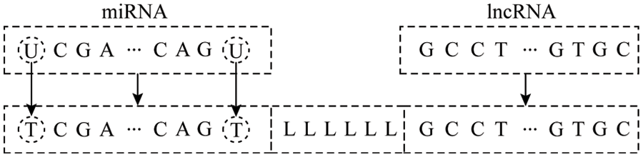
Figure 1: Relationship pair sequence

Because lncRNA sequences are substantially longer than miRNA sequences, lncRNA makes up a large amount of the integrated sequence. As a result, the total lncRNA is divided into those that participate in the interaction relationship and those that do not, with the Needleman-Wunsch algorithm being used to divide those that do not participate in the interaction connection. Compare the similarity between the lncRNA in the positive sample and the lncRNA in the negative sample, and discard the lncRNA samples with a similarity of more than 80% [18]. Finally, after the similarity has been removed, combine the lncRNAs that are not implicated in the interaction relationship with all miRNAs at random and proceed with the stages below. A negative set sample library is the result of the processing described in Fig. 1. A random sampling approach is used to achieve a balance of positive and negative samples, with the negative set consisting of samples equal to the number of positive samples.

3.2 Sequence Coding

For the integrated miRNA-lncRNA sequence, using the continuous representation of biological sequences in genomics, similar to the word segmentation in natural language processing [19], each sequence is divided into multiple sub-sequences (biological words). That is, every three consecutive bases are used as a subsequence, and there is no overlap between them. After word segmentation is performed on all the sequences in the positive and negative samples, a statistics of a biological word list with a size of 4 × 4 × 4 = 64 is obtained. According to the words in the biological sequence probability of appearing in, is coded from large to small, and each sequence sample can be embedded into an n-dimensional vector, which is the input format of the model. The specific coding method is shown in Fig. 2.

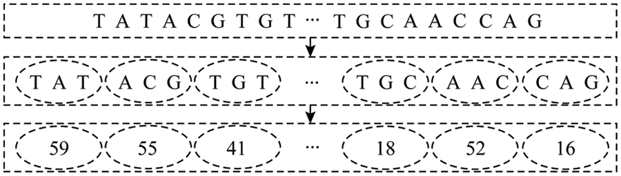
Figure 2: Coding order

As shown in Fig. 2, the input sequence S = (TATACGTGT…TGCAACCAG), according to the above scheme, every three consecutive bases are a word, and word segmentation is performed. Then coded according to the word frequency. Finally, after the program is run, the S is coded as a fixed length vector SC = (59, 55, 41, .., 18, 52, 16), i.e., a vector encoding a SC model last input format.

4  Proposed Model

The proposed model is mainly composed of an embedding stage, a convolution stage and a bidirectional LSTM stage.

4.1 Embedding Stage

The embedding stage is mainly to map the input sequence into a matrix vector form, and each column corresponds to a word. That is, each number in the input sequence is mapped into a vector with a fixed length, and the input sequence is mapped into a matrix form of m×n . Among them, m is the embedding vector dimension, n is the sequence length. The role of the embedding layer is to amplify some key features or separate some general features, and map the digital sequence into a matrix vector form that is easy to handle in the convolutional layer, which is convenient for subsequent volumes. Multilayer fully extracts features. For example, set the coding vector as SC = (19, 2, 30, 42, 28), after the embedding layer is used, it can be mapped into a matrix

SM=Embedding(SC)=[0.50.60.10.50.70.60.70.60.60.80.2−0.10.20.20.2−0.10.1−0.6−0.1−0.1−0.3−0.2−0.2−0.3−0.2] (1)

The parameters of the embedding layer in this experiment are that the input dimension is 66, the output dimension is 128, and the output length is 2840. That is, after the embedding layer, each sequence can be mapped into a 128 × 2840 vector as the input of the convolutional layer.

4.2 Convolution Stage

Since 1D convolution (Convolution1D) is mainly used for natural language processing, and 2D convolution (Convolution2D) is often used in computer vision [20], the experimental model convolution layer uses the Convolution1D function. The experimental convolution stage mainly consists of two convolutional layer composition. In addition, to prevent over-fitting, a dropout layer is added between the embedding and convolutional layer with a parameter of 0.5. The first layer of convolutional layer is convolution using 64 filters of length 10, which is equivalent to using sixty-four 10 × 128 convolution kernels to detect the matrix mapped by the embedded layer. That is, using the convolution kernel W to perform the matrix convolution operation:

xjh=f(xih−1∗Wj+bjh) (2)

Among them, xjh is the j th feature map, h represents the number of convolutional layers; Wj represents the j th convolution kernel; bjh represents the offset number of the j th feature map in the h th layer, and ∗ represents the convolution operation.

The RELU function is used to activate the convolutional layer because it has the advantages of enabling sparsity and successfully decreasing the gradient likelihood value compared to the sigmoid function [21] as follows:

RELU(x)=max(0,x) (3)

After the convolution operation, the feature map with a size of 64 × 2831 can be extracted. Then select MaxPooling with pool_length of 2 to sample the convolved features, that is, take the maximum value for the local area of the convolved feature, and extract the most important feature information. Therefore, the output dimension after the first convolution is 64 × 1415, which is used as the input of the next convolutional layer.

For example, use three 5 × 5 convolution kernels to convolve a 64 × 64 matrix to obtain three 60 × 60 feature maps, and then use a 2 × 2 pooling window for down-sampling. That is, three 30 × 30 feature mapping matrices and the specific convolution stage process is shown in Fig. 3.

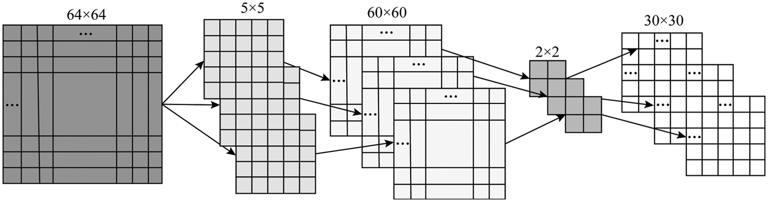
Figure 3: The convolution process

The second convolutional layer of the model uses 64 filters of length 5 to convolve, which is equivalent to re-convolving the features extracted from the upper layer with a 5 × 64 convolution kernel. Then the feature map size is extracted as 64 × 1411, after maximum pooling and sampling, a feature map with a size of 64 × 705 can be obtained, which is used as the input of the Bi-LSTM layer.

4.3 Bi-LSTM Stage

LSTM is a variant of RNN. It solves the problems of RNN gradient disappearance and gradient explosion and long-term dependence by setting input gates, forget gates, input gates and memory cells. However, one-way LSTM can only process information in one direction of the sequence. It cannot process information in the other direction. The Bi-directional RNN [22] can simultaneously capture the positive and negative direction information of the sequence, so as to better learn the characteristics of the sequence information. The Bi-LSTM is to solve the problem that LSTM can only handle a single direction to further expand the information, it learns from the bidirectional RNN method and replaces the cyclic unit in the bidirectional RNN with an LSTM unit. The Bi-LSTM is equivalent to a one-way LSTM connected before and after each training sequence, and these two one-way LSTMs are connected to the same layer, and feature information is extracted from the forward and reverse directions, which can fully learn more features. Fig. 4 is a two-way cyclic neural network [19].

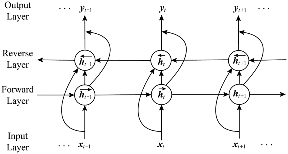
Figure 4: Illustration of Bi-RNN

Among them, the update formula of the neural network layer circulating from left to right is

h→t=H(Wxh→txt+Wh→h→h→t−1+bh→) (4)

The update formula for circulating the neural network layer from right to left is

h←t=H(Wxh←t+Wh←h←h←t+1+bh←)(5)

The output of the two layers of cyclic neural network layers before and after superimposed is n

yt=Wh→yh→t+Wh y←h←t+by(6)

Among them, t represents the time series; ht represents the hidden layer vector at time t, and the upper arrow represents the direction; xt represents the input at time t; yt represents the output at time t; Wxh represents the input-hidden layer weight matrix; Whh represents the hidden layer-hidden layer weight matrix; Why represents the hidden layer-output layer weight matrix; bh is the hidden layer bias vector; by is the output layer bias vector; H is the hidden layer activation function, where it select the sigmoid function.

The Bi-LSTM model transforms the information processing unit in Fig. 4 into an LSTM model unit, using LSTM memory cells to deal with long-term dependency loss, and combining the complementary information in the positive and negative directions to more fully learn the characteristics of the sequence data. Among them, in this experiment, the number of hidden layer neurons in Bi-LSTM is 64, and the dropout parameter is set to 0.3.

4.4 Model Implementation

The experimental model is based on TensorFlow 1.12.0 and written in Python 3.6.5 on a Windows 10 machine. The model is mainly composed of seven layers. The model first uses the embedding layer to map the input sequence into a 128 × 2840 matrix vector to facilitate the convolution operation. Followed by the use of a dropout layer with a parameter of 0.5 to prevent overfitting. Convolution through two convolution layers Operate and use the maximum pooling operation to filter out the important local feature information. After being excited by the RELU function, the rectangular vector is transformed into a 64 × 705-dimensional feature map as the input of the Bi-LSTM layer. The Bi-LSTM is combined with the context information advantage is to fully learn the dependencies between the features, and turn the feature mapping vector output in the convolution stage into a 128-dimensional vector. Finally, use the dense layer with a parameter of 1 to map the feature vector output by the Bi-LSTM into a specific use the sigmoid function to map the number between [0,1] to obtain the prediction result. According to the loss between the true value and the predicted value, the BP algorithm is used to calculate layer by layer, update the parameters, and complete a round of training. The overall structure of the model is shown in Fig. 5.

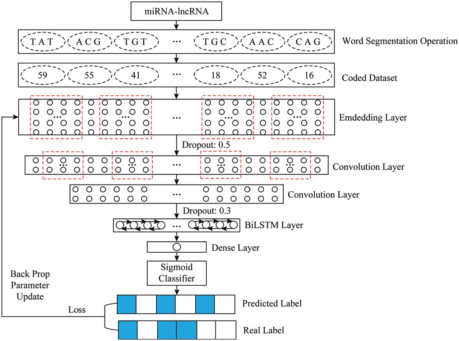
Figure 5: Overall framework of the proposed system

5  Experimental Results

Based on the corn (zea mays), potato (solanum tuberosum) and wheat (triticum aestivum) datasets, the traditional machine learning methods and different species are tested to verify the prediction ability and generalization of the proposed model for the miRNA-lncRNA interaction relationship ability.

5.1 Verification Methods and Evaluation Criteria

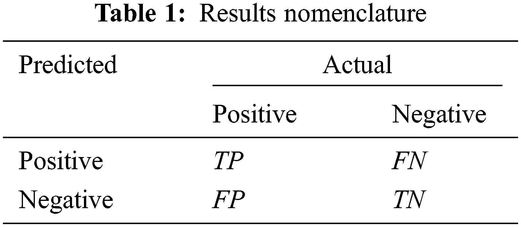
The experiment uses a 5-fold cross-validation method to verify the performance of the model. The idea of 5-fold cross-validation is to divide the data set into fie equally, take one of them in turn as the validation set, and the remaining 4 as the training set, and the average of the 5 results as Final evaluation value. The experiment selects accuracy (Acc), precision (P), recall (R) and F1 score (F1_score) as evaluation indicators:

Acc=TP+TNTN+TP+FP+FN (7)

P=TPTP+FP (8)

R=TPTP+FN (9)

F1=2×TP2×TP+FN+FP (10)

Among them, the meanings of TP, FP, TN, FN are shown in Tab. 1.

5.2 Data Set

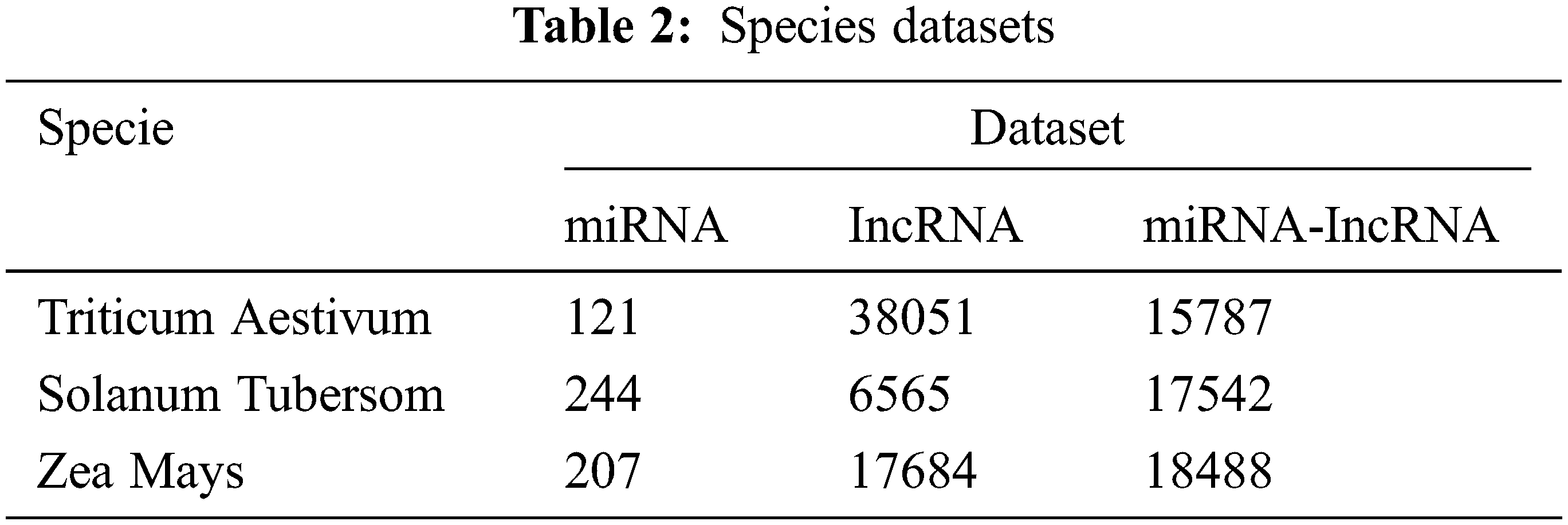
According to the method introduced in Section 3, download the relevant data of corn, potato and wheat from GreeNC and miRBase database, and proceed with the data preprocessing process of Section 3. First, use the corn data set, deployed traditional machine learning methods, single model to verify the effectiveness of the proposed method. In addition, using potato and wheat as data sets, the proposed model is used to conduct independent tests on the two to verify the generalization ability. In order to ensure the balance of positive and negative samples, randomly select the same number of samples as the positive set from the negative set sample library as the negative set. The specific data of each species data set is shown in Tab. 2.

5.3 Feature Extraction

Based on the traditional extraction methods of miRNA and lncRNA [23], the relevant features of maize miRNA and lncRNA are extracted respectively, and the two features are formed into a multi-dimensional feature set as the feature vector of machine learning.

First, use the RNAfold software in ViennaRNA [24] to obtain the minimum free energy (MFE) released when the lncRNA sequence forms the secondary structure and the dot bracket form of its secondary structure [25], and extract the number of paired bases and (C+G) base from it. Base content and the ratio of G, C, we can get the minimum free energy MFE, the number of paired bases n_pairs, (C+G) content CG_content and GC_ratio four features, the fusion feature is marked as Feature1:

CG_content=(Cnum+Gnum)/L (11)

GC_ratio=G_num/C_num (12)

Feature1=[MFE,npairs,CG_content,GC_ratio] (13)

Among them, C_num is the number of base C in the sequence; G_num is the number of base G in the sequence; L is the length of the sequence.

In addition, the k-mers feature of lncRNA is also extracted. A k-mers consists of k bases, then 1-mer = {A, T, C, G} has four kinds, 2-mer = {AA, AT, AC, AG,…}, each base can be A, T, C or G, so there are 4 × 4 = 16 types, in the experiment, k = 1, 2. The method of k-mers extraction is to use length along the lncRNA sequence sliding window of k is sliding matching with a step length of 1 base, then:

hi=wkmisk,k=1,2;i=1,2,…,20; (14)

sk=l−k+1,k=1,2; (15)

wk=143−k,k=1,2 (16)

Among them, wk is the weight; sk is the total number of matches; l is the length of the sequence; mi is the number of matches of each k-mers; hi is the frequency of each k-mers, then 4 + 16 = 20 of lncRNA can be obtained k-mers features, denoted as Feature2:

Feature2=[h1,h2,…,h20] (17)

The extracted features of miRNA sequence are the sequence length ml and the k-mers feature of miRNA, where k = 1, 2. Then 1 + 4 + 16 = 21 miRNA features can be obtained, denoted as Feature3:

Feature3=[ml,mh1,mh2,…,mh20] (18)

Finally, the features of lncRNA Feature1, Feature2 and miRNA feature Feature3 form a 4 + 20 + 21 = 45-dimensional feature set, which is used as the feature vector of traditional machine learning Feature:

Feature=(Feature1,Feature2,Feature3) (19)

5.4 Comparative Analysis

In order to verify the effectiveness and advantages of the proposed method, the experiment uses maize as the data set, extracts and fuses the features of miRNA and lncRNA according to the method in Section 4.3, and uses Naive Bayes (NB) [26], gradient boosting decision tree (GBDT) [27], random forest (RF) [28] and decision tree (DT) [29] methods for classification prediction, comparative experiments, 5-fold cross-check [30]. The experimental results are shown in Tab. 3.

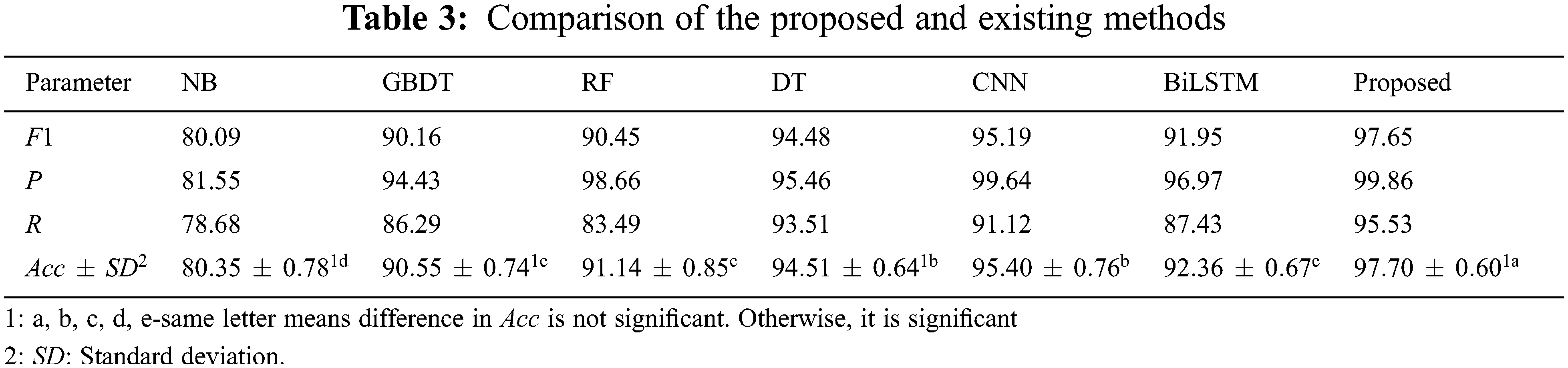
It can be seen from Tab. 3 that compared with traditional machine learning methods, the proposed method has obvious advantages in terms of accuracy, precision, recall, and F1 value. Among them, the accuracy is better than NB, GBDT, RF and DT methods are 17.35%, 7.15%, 6.56% and 3.19% higher respectively, indicating that the proposed method has a good classification ability in predicting the interaction between miRNA-lncRNA. At the same time, compared with the single model CNN and Bi- LSTM, the proposed model takes into account the advantages of both, which can extract rich features and solve the problem of long-distance information dependence, which is slightly better than the performance of a single model [31,32]. In addition, from the analysis results of the least significant difference (LSD) method, the proposed method is significantly better than other methods, and the standard deviation (SD) of accuracy is only 0.60%, indicating that the proposed model is stable [33,34].

Fig. 6 depicts the region of convergence (ROC) curve under different methods on the corn test set. From the results, it can be seen that compared with the machine learning model and the single model, the area under the ROC curve of the fusion model is the largest, and its area, that is, the area under the ROC curve (AUC) value is as high as 0.99 or more. Almost close to 1, very close to the real situation, indicating that the classification effect of the model is very significant.

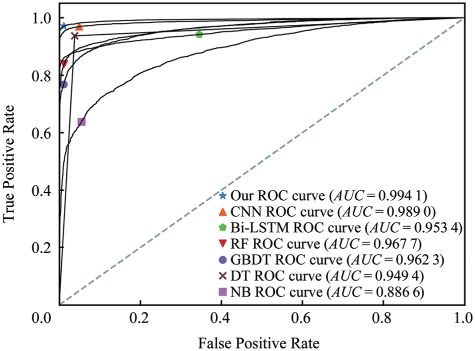
Figure 6: Comparison of TP and FP of the proposed and existing algorithms

5.5 Comparison of Species Classification

In order to prove the generalization ability of the proposed method, potato and wheat data sets are selected as independent test sets to conduct model tests. The experimental results of two different species prove that the proposed method has good generalization ability and is suitable for most species. The 5-fold cross test results are shown in Tab. 4.

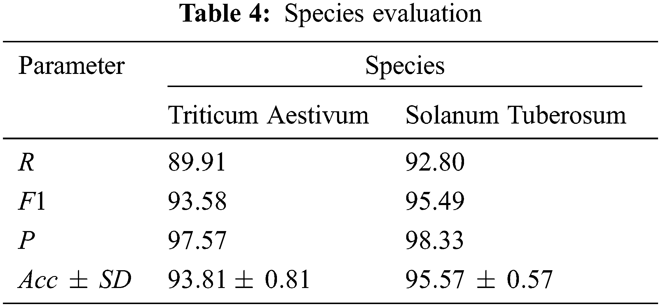
It can be seen from the results in Tab. 4 that the proposed method has good performance indicators in all aspects of predicting the interaction between miRNA-lncRNA of potato and wheat, indicating that the model has good generalization ability and is suitable for most species. In addition, both The variances of are all small, indicating that the stability of the model is also better under different species data.

6  Conclusion

This paper proposes a deep learning model that combines CNN and Bi-LSTM, taking into account the advantages of CNN and Bi-LSTM, fully considering the correlation between sequence data and better combining context information, so as to fully extract features. Experimental results show that the proposed model has a better classification effect than traditional machine learning and single model compared with traditional machine learning and single model. In addition, independent tests on potato and wheat data sets have also achieved good classification results, verifying the proposed model has good generalization ability and is suitable for testing most species.

In the future, we will try to use more models, such as capsule networks, deep belief networks, etc., to further improve the prediction of miRNA-lncRNA interaction. In addition, combining machine learning and deep learning methods to improve the prediction performance is also a future research direction.

Acknowledgement: The authors extend their appreciation to King Saud University for funding this work through the Researchers Supporting Project (No. RSP-2021/395), King Saud University, Riyadh, Saudi Arabia.

Funding Statement: This work was supported by the Researchers Supporting Project (No. RSP-2021/395), King Saud University, Riyadh, Saudi Arabia.

Conflicts of Interest: The authors declare that they have no conflicts of interest to report regarding the present study.

References

 1.  S. Schmitz, “Mechanisms of long noncoding RNA function in development and disease,” Cellular and Molecular Life Sciences, vol. 73, no. 13, pp. 2491–2509, 2016. [Google Scholar]

 2.  J. Wang, Y. Yang, Y. Ma, F. Wang, A. Xue et al., “Potential regulatory role of incRNA-miRNA-mRNA axis in osteosarcoma,” Biomedicine & Pharmacotherapy, vol. 121, no. 8, pp. 10123–10134, 2020. [Google Scholar]

 3.  A. Abugabah, A. A. AlZubi, M. Al-Maitah and A. Alarifi, “Brain epilepsy seizure detection using bio-inspired krill herd and artificial alga optimized neural network approaches,” Journal of Ambient Intelligence and Humanized Computing, vol. 12, no. 3, pp. 3317–3328, 2021. [Google Scholar]

 4.  J. Hui, M. Rong and Z. Shubiao, “Reconstruction and analysis of the lncRNA-miRNA-mRNA network based on competitive endogenous RNA reveal functional lncRNAs in rheumatoid arthritis,” Molecular Biosystems, vol. 13, no. 6, pp. 1182–1192, 2017. [Google Scholar]

 5.  S. Kim, J. Nam and J. Rhee, “miTarget: MicroRNA target gene prediction using a support vector machine,” BMC Bioinformatics, vol. 7, no. 1, pp. 411–423, 2006. [Google Scholar]

 6.  E. Asgari and K. Mofrad, “Continuous distributed representation of biological sequences for deep proteomics and genomics,” Plos One Journal, vol. 10, no. 11, pp. 871–882, 2015. [Google Scholar]

 7.  J. Cheng, P. Wang and G. Li, “Recent advances in efficient computation of deep convolutional neural networks.” Frontiers of Information Technology & Electronic Engineering, vol. 19, no. 1, pp. 64–77, 2018. [Google Scholar]

 8.  S. Hochreiter and J. Schmidhuber, “Long short-term memory,” Neural Computation, vol. 9, no. 8, pp. 1735–1780, 1997. [Google Scholar]

 9.  Y. Huang, X. Wang, Y. Zheng, W. Chen, Y. Zheng et al., “Construction of an mRNA-miRNA-lncRNA network prognostic for triple-negative breast cancer,” Aging Journal, vol. 13, no. 1, pp. 1153–1175, 2021. [Google Scholar]

10. H. Siyu, Y. Liang and Y. Li, “Long noncoding RNA identification: Computing machine learning based tools for long noncoding transcripts discrimination,” BioMed Research International, vol. 16, pp. 1–14, 2016. [Google Scholar]

11. M. Al-Maitah and A. A. AlZubi, “Enhanced computational model for gravitational search optimized echo state neural networks based oral cancer detection,” Journal of Medical Systems, vol. 42, no. 8, pp. 205–217, 2018. [Google Scholar]

12. R. Williams and D. Zipser, “A learning algorithms for continually running fully recurrent neural networks,” Neural Computation, vol. 1, no. 2, pp. 270–280, 1989. [Google Scholar]

13. R. Tripathi, S. Patel and V. Kumari, “DeepLNC: A long noncoding RNA prediction tool using deep neural network,” Network Modeling Analysis in Health Informatics and Bioinformatics, vol. 5, no. 1, pp. 5027–5034, 2016. [Google Scholar]

14. B. Junghwan, L. Byunghan and K. Sunyoung, “lncRNnet: Long non-coding RNA identification using deep learrning,” Bioinformatics, vol. 34, no. 22, pp. 3889–3897, 2018. [Google Scholar]

15. G. Andreau, H. Pulido and D. Irantzu, “A Wiki-based database of plant lncRNAs,” Nucleic Acids Research Journal, vol. 44, no. 1, pp. 1161–1166, 2016. [Google Scholar]

16. S. Griffithsjones, “miRBase: The microRNA sequence database,” Methods in Molecular Biology, vol. 342, no. 7, pp. 129–138, 2006. [Google Scholar]

17. X. Dai, Z. Zhuang and P. Zhao, “psRNATarget: A plant small RNA targer analysis server,” Nucleic Acids Research, vol. 46, no. 9, pp. 49–54, 2018. [Google Scholar]

18. T. Negri, W. Alves and P. Bugatti, “Pattern recognition analysis on long noncoding RNAs: A tool for prediction in plants,” Briefings in Bioinformatics, vol. 20, no. 2, pp. 682–689, 2019. [Google Scholar]

19. D. Shao, Z. Yang, Z. Chen, Y. Xiang, X. Yantuan et al., “Domain-specific Chinese word segmentation based on bi-directional long-short term memory model,” IEEE Access, vol. 7, pp. 12993–13002, 2019. [Google Scholar]

20. X. Tang, X. Zhang, F. Liu and L. Jiao, “Unsupervised deep feature learning for remote sensing image retrieval,” Remote Sensing, vol. 10, no. 8, pp. 1–27, 2018. [Google Scholar]

21. A. A. AlZubi, A. Alarifi and M. Al-Maitah, “Deep brain simulation wearable IoT sensor device based Parkinson brain disorder detection using heuristic tubu optimized sequence modular neural network,” Measurement, vol. 161, no. 3, pp. 1759–1768, 2020. [Google Scholar]

22. M. Schuster and K. Paliwal, “Bidirectional recurrent neural network,” IEEE Transactions on Signal Processing, vol. 45, no. 11, pp. 2673–2681, 1997. [Google Scholar]

23. X. Wang, J. Zhang and F. Li, “MicroRNA identification based on sequence and structure alignment,” Bioinformatics, vol. 21, no. 18, pp. 3610–3614, 2005. [Google Scholar]

24. R. Lorenz, S. Bernhart and C. Siederdissan, “ViennaRNA package 2.0,” Algorithms for Molecular Biology, vol. 6, no. 2, pp. 674–683, 2011. [Google Scholar]

25. J. Li, X. Zhang and C. Liu, “The computational approaches of lncRNA identification based on coding potential: Status quo and challenges,” Computational and Structural Biotechnology Journal, vol. 18, no. 4, pp. 3666–3677, 2018. [Google Scholar]

26. C. Gao, Q. Cheng and H. Pei, “Privacy-preserving naïve Bayes classifiers secure against the substitution-then-comparison attack,” Information Sciences, vol. 444, no. 10, pp. 72–88, 2018. [Google Scholar]

27. A. Alarifi and A. A. AlZubi, “Memetic search optimization along with genetic scale recurrent neural network for predictive rate of implant treatment,” Journal of Medical Systems, vol. 42, no. 11, pp. 202–216, 2018. [Google Scholar]

28. F. Rodriguez, B. Ghimire and J. Rogan, “An assessment of the effectiveness of a random forest classifier for land-cover classification,” ISPRS Journal of Photogrammetry & Remote Sensing, vol. 67, no. 1, pp. 93–104, 2012. [Google Scholar]

29. D. Landgrebe, “A survey of decision tree classifier methodology,” IEEE Transactions on Systems Man & Cybernetics¸, vol. 21, no. 3, pp. 660–674, 2002. [Google Scholar]

30. S. D. Ali, J. H. Kim, H. Tayara and K. Chong, “Prediction of RNA 5-hydroxymethylcytosine modifications using deep learning,” IEEE Access, vol. 9, pp. 8491–8496, 2021. [Google Scholar]

31. H. Tayara and K. Chong, “Improved predicting of the sequence specificities of RNA binding proteins by deep learning,” IEEE/ACM Transactions on Computational Biology and Bioinformatics, vol. 18, no. 6, pp. 2526–2534, 2021. [Google Scholar]

32. X. Gao, J. Zhang, Z. Wei and H. Hakonarson, “Deeppolya: A convolutional neural network approach for polyadenylation site prediction,” IEEE Access, vol. 6, pp. 24340–24349, 2018. [Google Scholar]

33. R. Zhang, W. F. Zhang, W. Sun, X. M. Sun and S. K. Jha, “A robust 3-D medical watermarking based on wavelet transform for data protection,” Computer Systems Science & Engineering, vol. 41, no. 3, pp. 1043–1056, 2022. [Google Scholar]

34. R. Zhang, X. Sun, X. M. Sun and S. K. Jha, “Robust reversible audio watermarking scheme for telemedicine and privacy protection,” Computers, Materials & Continua, vol. 71, no. 2, pp. 3035–3050, 2022. [Google Scholar]