Prediction of Suitable Crops Using Stacked Scaling Conjugant Neural Classifier

1  Introduction

Development of productivity in agriculture needs a seasonal approach for selecting the crops to cultivate. However, farmers don’t have the right supportive farm factors for cultivation based on environmental conditions. The selection of suitable crops for cultivation is one of the significant issues in the agriculture domain. So, an effective machine learning model could be used to solve the problem against improper seasonal recommendations to farmer. The seasonal crop data and seasonal weather data such as temperature, humidity, sunlight, and related factors are aggregated for analysis. Fig. 1 shows the process of crop recommendation. Climatic change affects the agricultural sector massively, because of its direct dependence on the weather. The nature and extent of these effects impact rely not only on the evolution of the climatic system but also on crop yield and weather conditions.

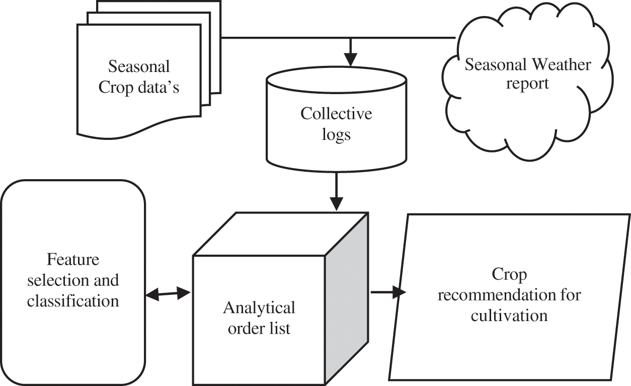
Figure 1: Process of crop recommendation

Based on crop meteorological studies, crop yield forecast samples were taken to estimate the yield of several crops before the actual harvest. In addition, meteorological research parameters are used to model different crop growth stages in conjunction with technological trends. This work intends to create a model for obtaining feature selection based on radial features from the seasonal datasets.

2  Related Works

In general, the neural network predicts the decision class of unseen associations. However, it may fail if the information system is quantitative because the attribute values are almost indistinct, and the information system may not be deterministic. The uncertainties are overwhelmed by hybridizing rough sets on fuzzy approximation space and neural backpropagation networks. The rough set on fuzzy approximation space identifies the almost indiscernibility among the natural resources. It helps in minimizing the computational procedure of employing data reduction techniques, whereas neural network helps in the prediction process [1]. This model is put to use in the analysis of the agricultural data of Vellore District, Tamil Nadu, India. The Bayesian model for crop yield increases modelling flexibility and improves prediction over existing least-squares methods [2]. The developed model focuses on a more accurate forecast with reduced noise. In addition, dimension-reduction schemes are examined to improve prediction. A linear method such as linear regression is insufficient to show the interactions of the factors and crop yield. The application of artificial intelligence in the agricultural sector will become a more exciting research area of interest and has high potential [3]. A Crop Selection Method (CSM) is developed using Artificial Neural Network (ANN) to select a sequence of crops planted over the season. It is based on predicting the yield rate influenced by various parameters such as weather, soil type, water density, and crop type. It takes crop, sowing time, plantation days, and predicted yield rate for the season as input and suggests a sequence of suitable crops. The CSM method improves the net yield rate of crops planted over the season. Data mining techniques predict the crop yield based on the climatic input parameters [4].

Agriculture development depends on different parameters: water, weather, soil characteristics, crop rotation, soil moisture, surface temperature, rainfall, etc. In India, the agriculture growth depends on rainwater, which is highly unpredictable. Various regression models like Linear, Multiple Linear, and Non-linear models are tested for effective prediction to forecast the agriculture yield for multiple crops in Andhra Pradesh and Telangana states [5]. An integrated prediction model was developed, a linear combination of the three ensemble members using Bayesian Model Averaging (BMA) weights. It evaluates the impact of climate change and agricultural management on crop growth [6]. This integrated approach results in more accurate and precise predictions than the individual model. The interpretation of the BMA weight values is also strengthened by comparing regional precipitation, fertilization, and radiation data.

A non-parametric statistical model was developed, which focuses on processing weather data and configuring the prediction system [7]. It takes Meteorological data as the inputs of modelling and generates the secondary meteorological data to reflect the characteristics of the plant. Machine learning is an imminent field of computer science that can be applied to the farming sector effectively. It can simplify the up-gradation of conventional farming techniques in the most cost-effective approach [8].

An advanced technology called Weighted-Self Organizing Map (W-SOM) is employed for an accurate crop and weather prediction, which is the combination of both Self Organizing Map (SOM) and Learning Vector Quantization (LVQ) [9]. The prediction accuracy is enhanced by minimizing the Within Class Error (WCE) among the clusters. This approach has given a clear decision about suitable crop cultivation in Mysore. The selection of crops before the plantation has a vital role in farming, because the yield is mainly depended on the crop selected for cultivation and environmental parameters [10].

In Agriculture, loss occurs due to the false selection of crop for cultivation on a particular land. The farmers are generally not aware of the requirements of the crop, i.e., the minerals, soil moisture, and other soil requirements. A model is developed which predicts the best suitable yield for the farmer and detects the pest that may affect as well [11]. Support Vector Machine (SVM) classification algorithm, Decision Tree algorithm, and Logistic Regression algorithm were applied, and the SVM classification model gives better accuracy than other algorithms. With data mining, crop yield can be predicted by springing valuable insights from the agricultural data that aid farmers in deciding the crop they should plant, which in turn leads to maximizing the profit [12]. The gray prediction method [13] is used to predict the price of agricultural products in the market. A time-spectral approach [14] used to model a time domain in Numeric Weather Prediction (NWP). Regular rainfall patterns are usually important for healthy agriculture, but high or low rainfall rate can be harmful and even destroy crops [15]. A mobile phone based crowdsourcing approach was proposed to classify pest and diseases in a region by aggregating information from multiple farmers [16]. Lightweight convolutional neural network with feature optimization and a joint learning strategy is proposed to reduce network parameters and improve classification accuracy [17].

3  Materials and Method

The proposed model suggests the crops based on the historical data. Approaching crop sample forecasts based on weather-related data can encourage the farmers to focus on the most suitable crops rather than planting any other crop. The proposed crop production model may consist of two main stages, specifically feature selection and classification.

Fig. 2 shows the proposed architecture for recommending more suitable crops by selecting the more significant features and performing classification.

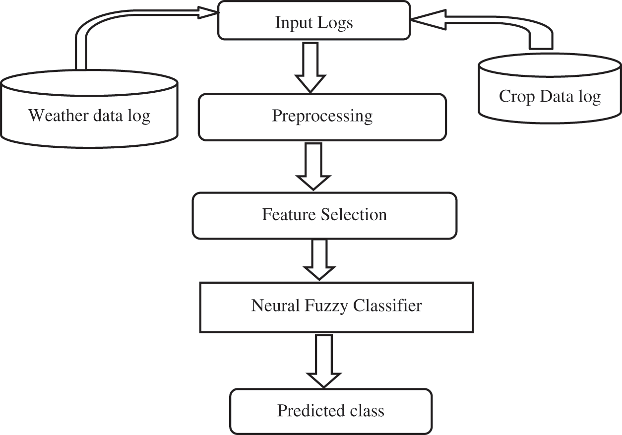
Figure 2: Proposed architecture

3.1 Data Collection Phase

In the Data collection phase, a wide range of weather-related data is collected from south Asia datasets. Furthermore, the proposed crop recommendation model is analyzed with crops like rice, wheat, jowar, bajra, muskmelon, corn, maize, ragi and pulses. The historical data for analyzed crops were also gathered. The harvest data modules contain the details about harvest, weather, soil, rainfall, moisture, temperature, crop cost, crop type data etc. Fig. 3 shows the crop dataset collective features. The seasonal weather data and crop data are collected and aggregated for analysis.

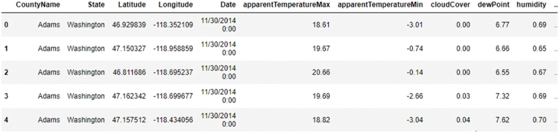
Figure 3: Crop dataset collective features

3.2 Preprocessing

The majority of real-world data has noise, missing values, and is in an inadequate format that cannot be directly used in machine learning models. Data preprocessing is a necessary task for cleaning data and making it suitable for a machine learning model, which improves the model’s accuracy and efficiency. Preprocessing removes the null field, non-range values, and noisy data to make it clean and formatted. Next, each data verification and validation are done in stages. Finally, each record set is ordered by index feature value, getting the list of features in redundant form.

Algorithm: preprocessing dataset

Step 1: Start

Step 2: Initialize the crop recommended forecasting Crf and weather dataset Wd

Step 3: Input dataset Crf→cr1, cr2, cr3 + wd (Index + 1)

Step 4: For (Crs combines attributes as feature Fi)

Step 5: Check →Null field if Yes

    Terminate record and update recordsetRcs.

   Else

    return

   Return Rcs←Crf+Wd;

   End if; End for;

Step 6: Compute Duplicate and non-fill case (Fls) and Attribute range

Step 7: Remove duplicate if Rcs←Rd(Fls) attain Get range(Ar)

   End if

Step 8: Check if (Rcs!=Empty fill near average)

   Get All the future index count terms.

   Returns preprocess data set

     (P)=F(Crf+Wd)n=∑I=0n⁡(nk)Rcs.Update → get real index, where n is total dominant features with k observed feature.

   Return redundant feature set

   End if

Step 9: Stop

The above algorithm processes the original data and reduces the noise from the data set. The range of the values conditionally verifies the appropriate logical threshold margins to check the fittest margin.

3.3 Probabilistic Approach for Feature Selection

Let the training set be {xi, yi}, where each xi, i = 1, 2, 3…, n be the m dimensional vector representing m features f1, f2…, fm, n be the total number of training samples and yi be the equivalent class label taking the values i = 1, 2, 3,…, c where c indicate the number of classes in the data. Let ri, i = 0, 1, 2, 3,…, t be the score given to each feature in the data set according to the intensity of the feature, where t is an integer indicating the maximum score (highest intensity) of the feature. Let Nk denote the number of training instances in the kth class where k = 1, 2,…, c.

1.    For each class k, find the total number of scores tl, l = 0, 1, 2…, t corresponding to ri, i = 0, 1, 2…, t respectively for the jth feature, j = 1, 2, 3…, n.

2.    Calculate the total score given to each feature R=∑i=0tri

3.    For each feature the probability of ri, i = 0, 1, 2…, t for each class k, k = 1, 2, 3…, c be pri=tlNk , i = 0, 1, 2,.., t

4.    The probability of the jth feature for the class k be pk=∑i=0t((riR)pri) , k = 1, 2, 3…, c (∑i=0triR=1)

5.    Calculate the weight of jth feature for the class k as wk=nNk∑k=1c⁡nNk

6.    Weighted probability of the jth feature is pj = ∑k=ncwkpk , j = 1, 2,.., n

7.    Find the threshold for the entire training dataset, which is the average of the weighted probability of n features. i.e., T= ∑j=1mpjm .

8.    Arrange the features of weighted probabilities in the decreasing order.

9.    Set the base model as the subset of feature set to include features with weighted probabilities greater than the threshold value in the feature set.

Fig. 4 shows the dominant feature’s weightage from the weather dataset using probabilistic approach for feature selection.

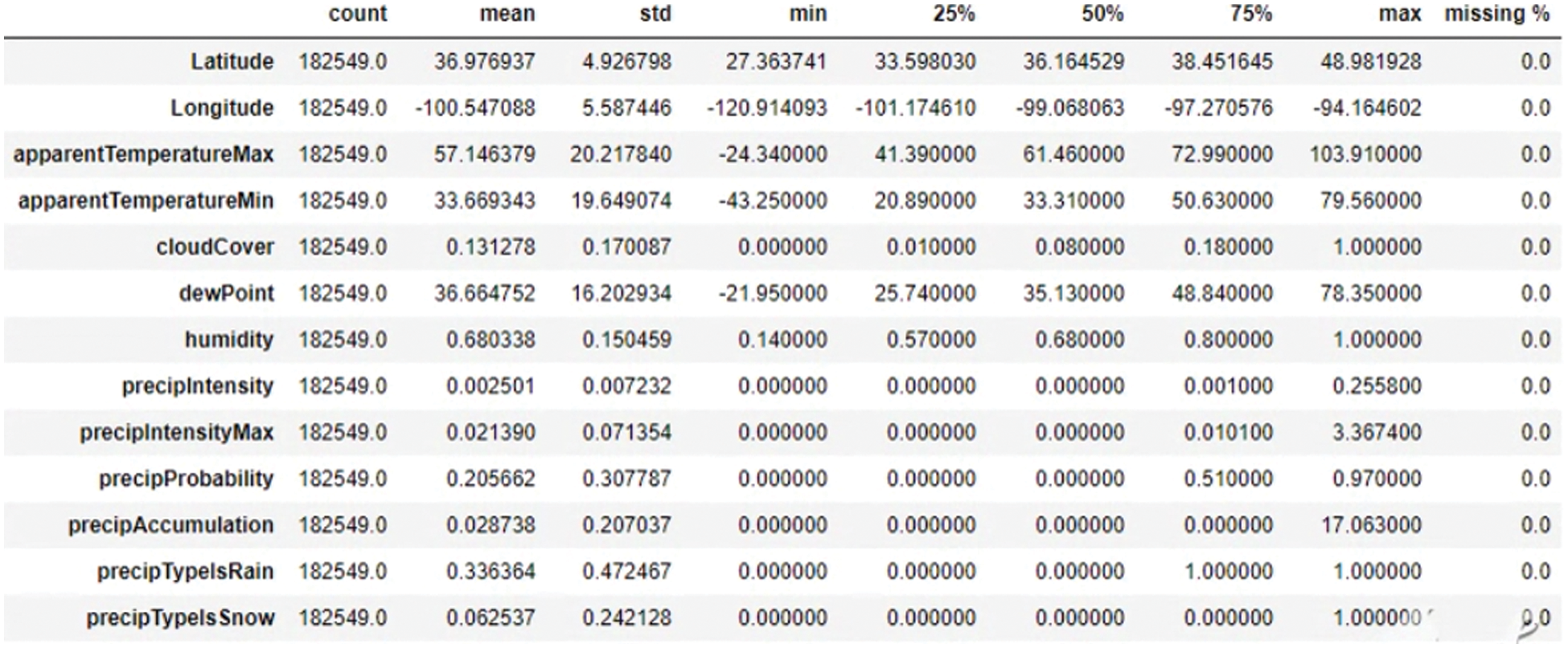
Figure 4: Dominant feature’s weightage

3.4 Neural Fuzzy Classifier (NFC)

The NFC divides the feature space into several fuzzy subspaces applying fuzzy if-then logic. A network structure can be used to express these fuzzy rules. There are several inputs and outputs for the classifier. It consists of layers such as input, fuzzy membership, fuzzification, defuzzification, normalization, and output.

The membership function of each input is identified in the membership layer. Gaussian function is used in this work because it has fewer parameters and smooth partial derivatives for parameters. Gaussian function is defined as.

μij(xsj)=exp(−(xsj−cij)22σij2) (1)

where μij(xsj) represent the membership value of ith rule and jth feature; xnj is the sth sample and jth feature; cij is the center and σij is the width of the width of the gaussian function.

In the fuzzification layer, each node generates a signal corresponding to the degree of membership for the sample xs as follows:

αis∏j=1Nμij(xsj (2)

The output weights are calculated in the defuzzification layer. For the sth sample in the kth class, the weighted output is determined as follows:

βsk=∑i=1Nαiswik (3)

where wik indicates the degree of membership to the kth class that the ith rule regulates, and N is the number of rules. The total of weights can be more than 1 in some circumstances, in such case the network outputs should be normalized.

osk=βsk∑l=1K⁡βsl (4)

where K is the number of classes and osk is the normalised value of the sth sample that corresponds to the kth class. Class label of a particular class is obtained by,

cs=k=1,2,3..K{osk}max (5)

where Cs represents the class label of sth sample.

3.5 Training the Classifier

To determine the optimum fuzzy region, the parameter θ of fuzzy rules must be optimized.

θ={CMXN,SMXN,WMXK} (6)

where K, M and N are the classes, rules and features respectively means clustering algorithm is used to obtain the initial parameters for forming the fuzzy rule. Scaling Conjugate Gradient learning method are used to update the weights. The classifier constructs neural network weightage by fuzzy membership function.

Eqw(y)=E(w)+E′(w)Ty+12yTE′′(w)y (7)

Critical points must be determined as follows to obtain a minimum error,

E′qw(y)=E′′(w)y+E′(w)=0 (8)

The time consumption for searching in every iteration is reduced, which makes the SCG algorithm faster than the second order algorithm. The result shows that the SCG algorithm provides least error and highest efficiency.

4  Result and Discussion

According to the proposed method, feature selection and classification has made. Then, the algorithm has evaluated with a confusion matrix. As a result, the proposed method produces better performance than the conventional method.

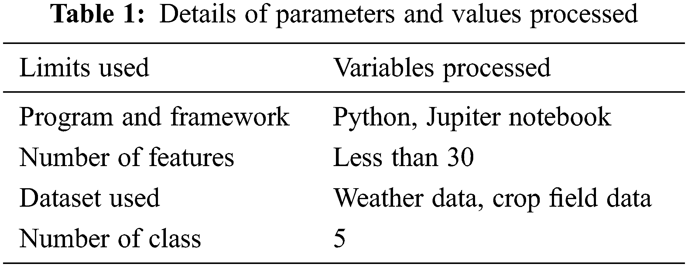
Tab. 1 shows the details of parameters and execution environment. Evaluation is done on the proposed model using evaluation metrics such as precision, recall, accuracy, and time complexity.

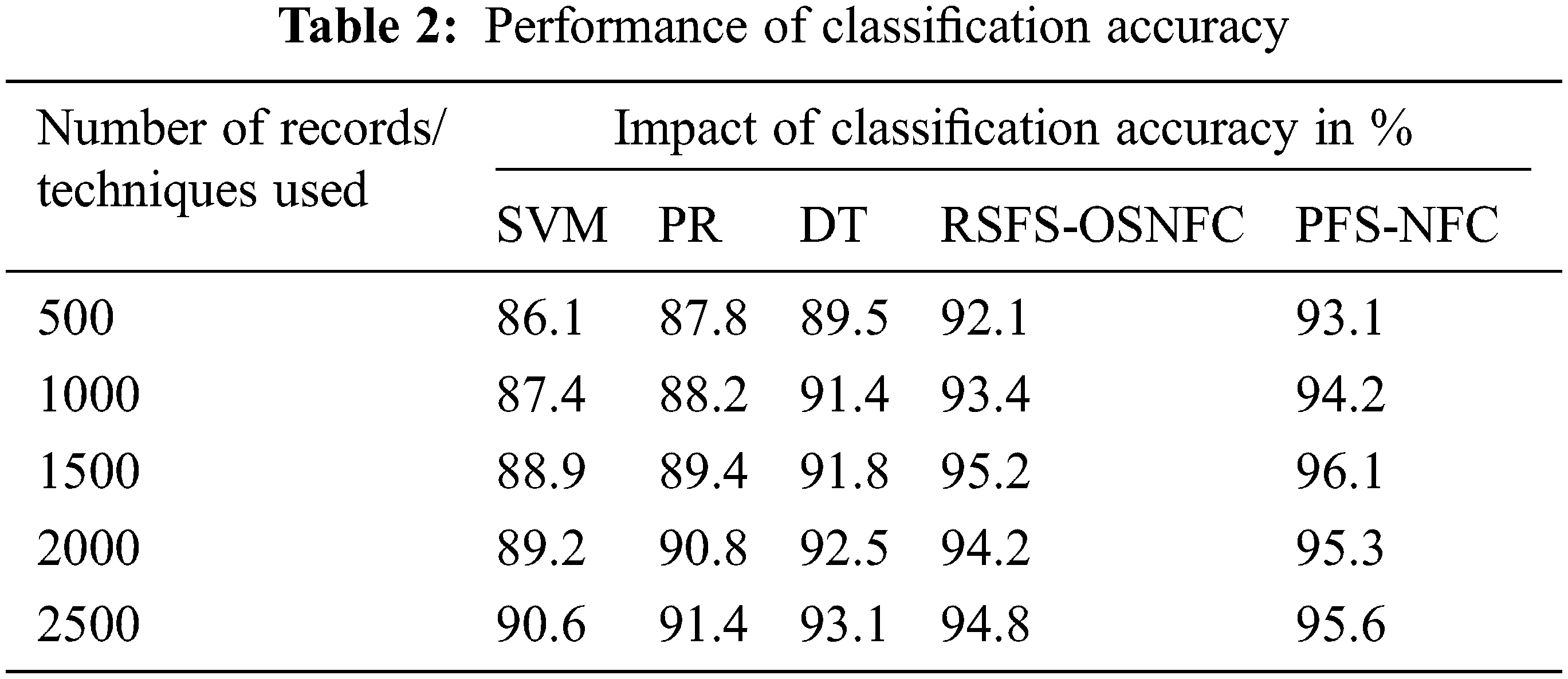
The proposed system provides high classification accuracy of 95.6% than the methods such as Support Vector Machines (SVM), Polynomial Regression (PR), and Decision Trees (DT) as shown in Tab. 2.

Accuracy can be calculated in terms of positives and negatives as follows,

    Accuracy=TN+TP (TP+FP+FN+TN ) (9)

The proposed model has higher classification accuracy than other methods, as shown in Fig. 5.

Figure 5: Performance of classification accuracy

As shown in Fig. 6, the accuracy of precision and recall rate checked with an average macro rate under the ratio of mean depth is estimated to produce the best accuracy. The marginal frequency is adjusted by the error rate based on the absolute error by support values.

Figure 6: Accuracy of precision recall rate

Sensitivity can be calculated as,

    Sensitivity=TP TP+FN (10)

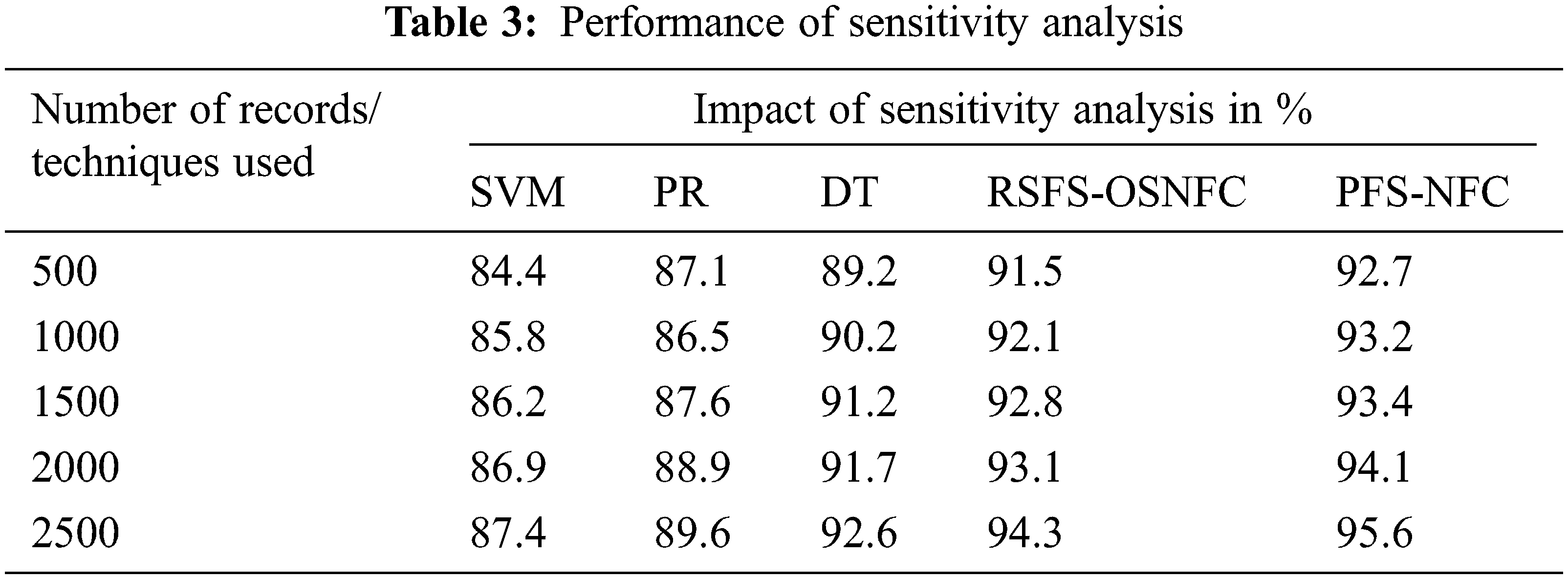
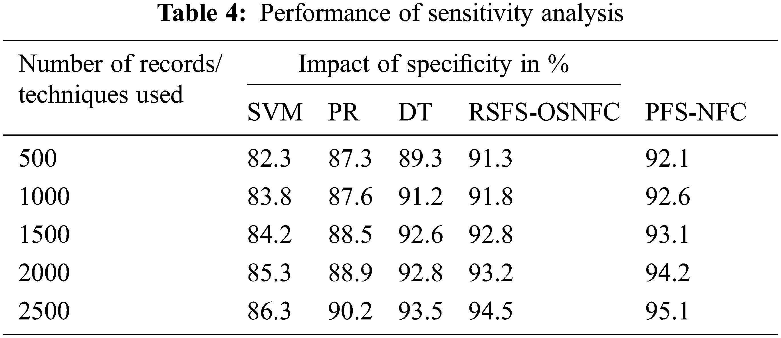
Fig. 7 shows the sensitivity analysis obtained by various models. The proposed system has better results of 95.6%.

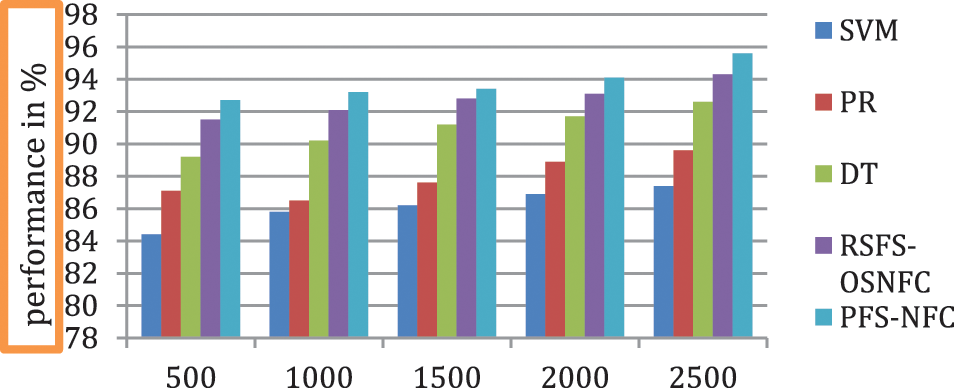
Figure 7: Performance of sensitivity analysis

Fig. 8 shows the sample result obtained by the proposed model.It predicts the suitable crop for cultivation by analyzing the input parameters.

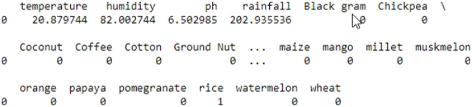
Figure 8: Recommended yield prediction class

Tab. 3 shows the impact of the sensitivity rate produced by different methods in which the proposed system has a higher sensitivity rate than other methods.

Specificity can be calculated as,

    Specificity=TNTN+FP  (11)

Fig. 9 shows the specificity analysis obtained by various models. The proposed method has higher performance than the other methods.

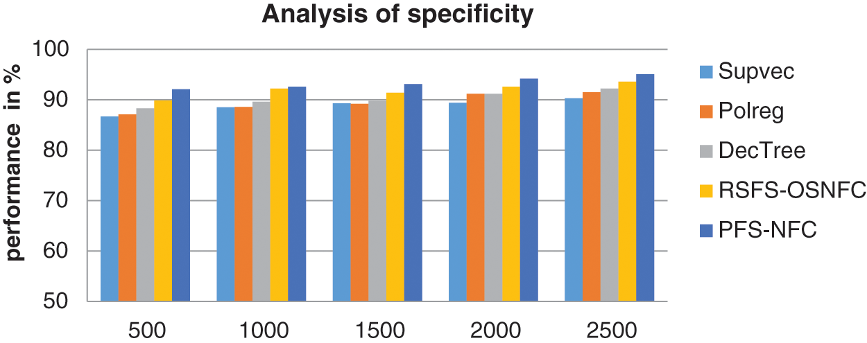
Figure 9: Performance of specificity

Tab. 4 shows the specificity rate achieved by different methods.

The F-measure is the harmonic mean of sensitivity and specificity. Fig. 10 shows the F-measure value achieved by all the models. F-measure can be calculated as,

F−Measure=(2∗Precision∗Recall)/(Precision+Recall) (12)

Figure 10: Performance of F-measure

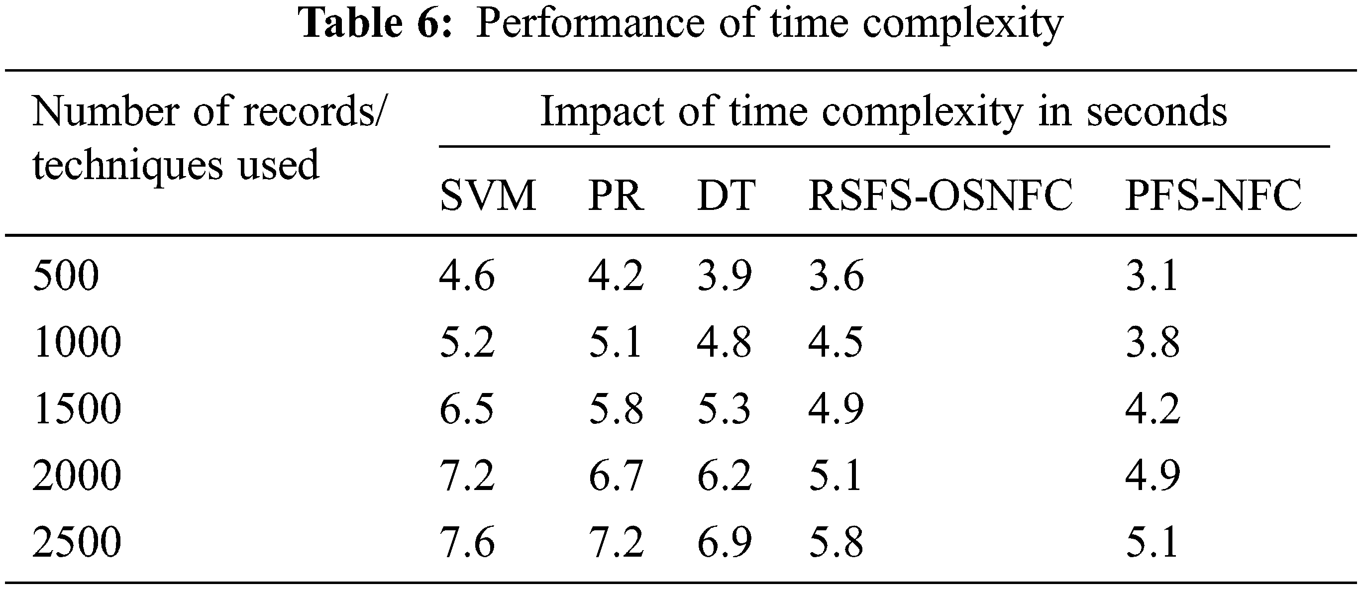
Tab. 5 demonstrates the F-measure value achieved by all the models. Time complexity denotes the time required to complete the task concerning the input size.

Time complexity (Tc)=∑k=0k=n×Total Features Handeled to Process in DatasetTime Taken(Ts) (13)

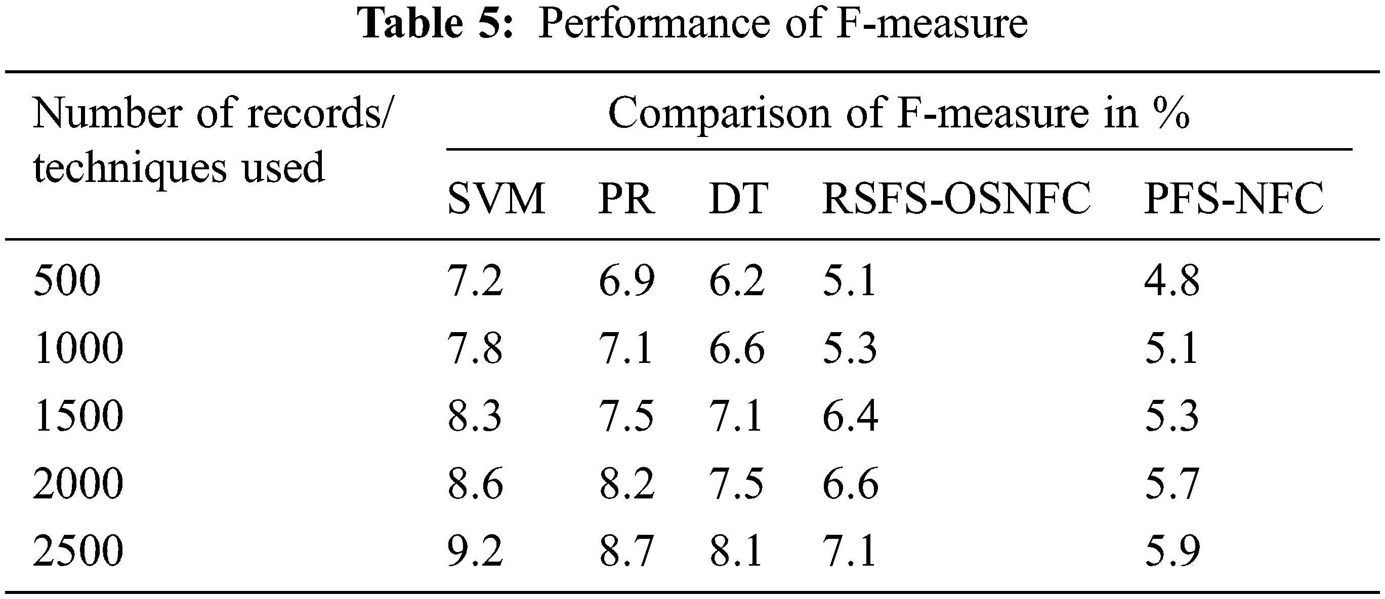
Fig. 11 shows the time complexity achieved by various models.

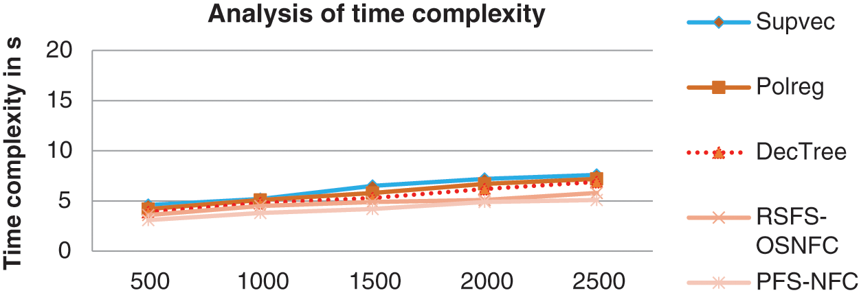
Figure 11: Time complexity

Tab. 6 shows the execution time details of different methods. The proposed method takes lower time complexity than the other methods.

5  Conclusion

This work predicts a suitable crop using feature selection and classification, which achieves 95.6% of accuracy. The proposed method achieves high accuracy in comparison with the other methods. This work would help farmers predict suitable crops based on the soil requirements before cultivation. Generally, the crop decision in the current position depends on the season influenced by the crop harvested during the last cycle. Hence it is planned to work with crop rotation prediction to maximize the yield in the future.

Availability of Data and Materials: Study uses Crop and weather dataset which is freely available at https://kaggle.com/.

Funding Statement: The authors received no specific funding for this study.

Conflicts of Interest: The authors declare that they have no conflicts of interest to report regarding the present study.

References

 1.  A. Anitha and D. P. Acharjya, “Crop suitability prediction in Vellore istrict using rough set on fuzzy approximation space and neural network,” Neural Computing & Applications, vol. 30, no. 12, pp. 3633–3650, 2018. [Google Scholar]

 2.  L. Bornn and J. V. Zidek, “Efficient stabilization of crop yield prediction in the Canadian prairies,” in The University of British Columbia, Department of Statistics, Technical Report #258, 2010 [Google Scholar]

 3.  R. Kumar, M. P. Singh, P. Kumar and J. P. Singh, “Crop selection method to maximize crop yield rate using machine learning technique,” in Int. Conf. on Smart Technologies and Management for Computing, Communication, Controls, Energy and Materials (ICSTM), Chennai, Tamil Nadu, India, 2015, pp. 138–145. [Google Scholar]

 4.  S. S. Veenadhari, B. Misra and C. Singh, “Machine learning approach for forecasting crop yield based on climatic parameters,” in 2014 Int. Conf. on Computer Communication and Informatics, Coimbatore, Tamil Nadu, India, pp. 1–5, 2014. [Google Scholar]

 5.  S. Nagini, T. V. Rajini Kanth and B. V. Kiranmayee, “Agriculture yield prediction using predictive analytic techniques,” in 2nd Int. Conf. on Contemporary Computing and Informatics (IC3I), Noida, UP, India, pp. 783–788, 2016. [Google Scholar]

 6.  X. Huang, G. Huang, C. Yu, S. Ni and L. Yu, “A multiple crop model ensemble for improving broad-scale yield prediction using Bayesian model averaging,” Field Crops Research, vol. 211, pp. 114–124, 2017, https://doi.org/10.1016/j.fcr.2017.06.011. [Google Scholar]

 7.  H. Lee and A. Moon, “Development of yield prediction system based on real-time agricultural meteorological information,” in 16th Int. Conf. on Advanced Communication Technology (ICACT2014), Phoenix Park, Pyeongchang Korea (southpp. 1292–1295, 2014. [Google Scholar]

 8.  K. Kauri, “Machine learning: Applications in Indian agriculture,” International Journal of Advanced Research in Computer and Communication Engineering, vol. 5, no. 4, pp. 35–38, 2016. [Google Scholar]

 9.  M. Pushpa and P. Kiran Kumari, “Weather and crop prediction using modified self organizing map for mysore region,” International Journal of Intelligent Engineering and Systems, vol. 11, no. 2, pp. 192–199, 2018. [Google Scholar]

10. N. Jain, A. Kumar, S. Garud, V. Pradhan and P. Kulkarni, “Crop selection method based on various environmental factors using machine learning,” International Journal of Advanced Research in Computer and Communication Engineering, vol. 8, no. 2, pp. 1530–1533, 2019. [Google Scholar]

11. A. Kumar, S. Sarkar and C. Pradhan “Recommendation system for crop identification and pest control technique in agriculture,” in Int. Conf. on Communication and Signal Processing (ICCSP), Chennai, Tamil Nadu, India, pp. 0185–0189, 2019. [Google Scholar]

12. H. Dhivya, R. Manjula, S. Siva Bharathi and R. Madhumathi, “A survey on crop yield prediction based on agricultural data”, International Journal of Innovative Research in Science, Engineering and Technology, vol. 6, no. 3, pp. 4177–4183, 2017. [Google Scholar]

13. J. Zong and Q. Zhu, “Apply grey prediction in the agriculture production price,” in Fourth Int. Conf. on Multimedia Information Networking and Security (MINES), Nanjing, Jiangsu, China, pp. 396–399, 2012. [Google Scholar]

14. J. Scheffel, K. Lindvall and H. F. Yik, “A Time-spectral approach to numerical weather prediction,” Computer Physics Communications, vol. 226, pp. 127–135, 2018. [Google Scholar]

15. T. Chandrasegar, K. Sri Harsha, M. Lakshmi Deepak and K. Chaitanya Krishna, “Heuristic prediction of rainfall using machine learning techniques,” in Int. Conf. on Trends in Electronics and Informatics (ICEI), Tirunelveli, Tamil Nadu, India, pp. 1114–1117, 2017. [Google Scholar]

16. P. Singh, B. Jagyasi, N. Rai and S. Gharge, “Decision tree based mobile crowd sourcing for agriculture advisory system,” in 2014 Annual IEEE India Conf. (INDICON), Pune, Maharastra, India, pp. 1–6, 2014. [Google Scholar]

17. W. Sun, G. Zhang and X. Zhang, “Fine-grained vehicle type classification using lightweight convolutional neural network with feature optimization and joint learning strategy,” Multimedia Tools and Applications, vol. 80, no. 20, pp. 30803–30816, 2021. [Google Scholar]