Enhanced Feature Fusion Segmentation for Tumor Detection Using Intelligent Techniques

1  Introduction

There are billions of cells in the brain, which is a very complicated structure that controls almost all of a person’s body’s work. A frenzied dissection of these single-cell parts is what causes a brain tumor that puts a person’s life in danger. The frantic movement of these single-cell parts causes the brain, which is the human body’s intelligent system, to break down. These growths also hurt the brain’s strong cell structures, as shown in Fig. 1a, which shows parts of the human brain with tumor cells. Outgrowths are often found in the area around the rinds of the human’s intelligent system (meninges), glands, or CNS (central nervous system), as shown in Figs. 1b and 1c. They cause even more damage to the brain cells by smearing constant compression inside the cranium, which spreads out the damage.

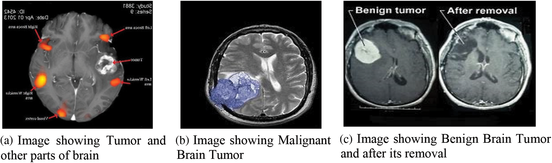
Figure 1: Brain Tumor and its varieties

There are two types of unnatural cell growth in the brain: benign and malignant, as shown in Figs. 1b and 1c. In most cases, benign (non-dangerous) tumor cells are marked with grades 1 and 2. Dangerous tumor cells are marked with grades 3 and 4. Non-cancerous outgrowth is usually referred to as a benign subtype because it is less aggressive and doesn’t grow. These start to grow inside the cranium, and they move at a snail’s pace. Grade I tumors [1] can be seen through a microscope, but grade II tumors look weird when viewed through a microscope. Both types of tumors are treated with surgery. Pilocytic astrocytoma, ganglioglioma, and gangliocytoma are examples of these types of tumors. When it comes to grade 3, which is cancerous and grows at an uncontrollable rate, there is a lot of variation from grade 2 and usually shows up as grade IV tumors. Secondary malignant tumors start in other parts of the body and travel to the brain to grow into secondary malignant tumors [2]. Primary malignant tumors start in the brain itself.

Tumors can have a big effect on how long people live. The high-grade subtype is a dangerous type that kills about 14,000 people a year. These irregular growths of cells in the brain cause pressure in the parts of the brain that are near them. These abnormalities make it hard for the brain to control the normal activities of the body. People who have these abnormalities have light-headedness, pain in the head, fall over, become paralysed, and so on to name a few. Grades 3 and 4 are more likely to damage the healthy tissues that surround the brain, and they often have to be fixed with surgery. To get rid of these bad groups of cells, doctors use things like drug therapy, particle emission therapy, and so on. In spite of a lot of work and progress in technology over the last few decades, people who have tumors still don’t live more than a few years. Computer Tomography (CT), X-rays, and Positron Emission Tomography (PET) are some of the imaging techniques used to find the abnormalities on the brain. There are also different types of Magnetic Resonance Imaging (MRI) techniques that can show these abnormalities. Few of the modes are shown in the Fig. 2 below.

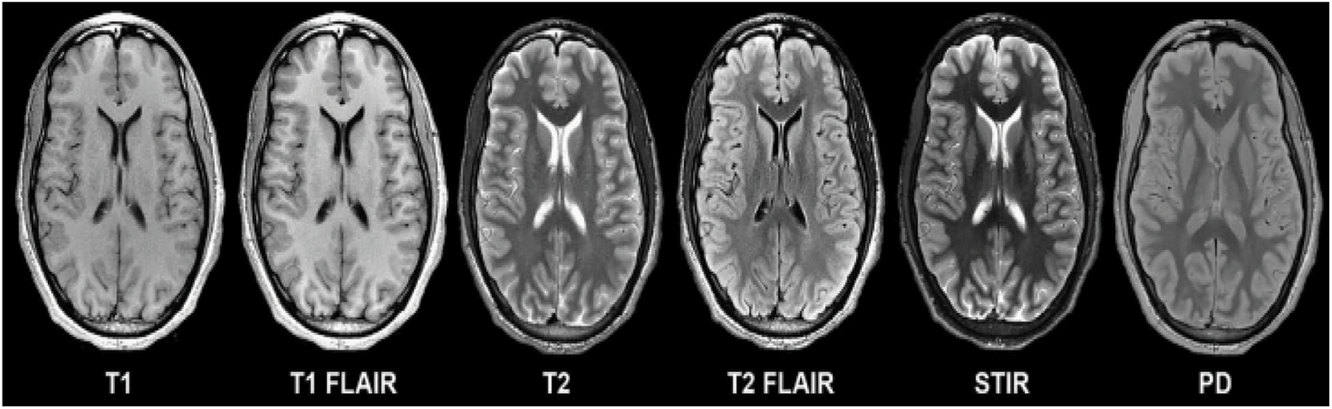
Figure 2: Various image modalities of brain

In Fig. 2, T1 and T2 are shown as weighted imaging, while T1 FLAIR and T2 FLAIR are shown as weighted Fluid Attenuated Inversion Recovery, which is what they are called. A multi-grade detection of the brain is a step toward understanding these problems, but there are still problems with segmentation accuracy and classification accuracy. There is a lot of noise, a lot of intensity variation, a lot of variation in tumor size, and a lot of other things that radiologist and computer vision researchers have to deal with. In clinical terms, imaging is the main tool used to look for abnormal cell growth in the brain. These imaging techniques give information about things like where the abnormal growth is and how dense it is, which helps surgeons a lot and also helps them see how well treatment is working. In addition to the above, they show quantitative image features like the variance and similarity between the intensity of nearby pixels [3]. Many scientists think that when they use this information with a machine learning algorithm, they will make great progress in the diagnosis and treatment of tumors. Machine learning studies in the past used a variety of steps to separate images into normal and abnormal ones. These steps included analysing the data, finding the most important features, and reducing the number of properties that were found so that the process was more efficient. Experts in the field, such as radiologists and doctors, were the ones who did the majority of the work in this area. It is a very clumsy and tiring thing to do for someone who isn’t very good at it. Extracting features from images is the first step in traditional machine learning. The accuracy of segregation is mostly dependent on the features that are retrieved. Thus, spotting a tumor in the brain’s complex composition is a very important process that is very much influenced by the way the brain is segmented. Radiologists used to do manual segmentation in the early days, but this took up a lot of their time, which made them want to use an automatic or semiautomatic process to find tumor cells.

There are a lot of people in the field of medicine who want a full-fledged automatic diagnostic system [4] that can tell the difference between tumor cells and non-tumor cells through MRI images. They use automated processes to help them improve their analysis skills with the help of automated machine learning mechanisms. These tools are good at giving you more information, but there are still problems with things like repeatable and accurate segmentation. Researchers are still having problems because there is a lot of variation in the area of interest, the shape, and the size of the tumor cell. These above mentioned challenges motivated in devising the proposed mechanism to develop a fully automatic method to escalate the detection performance with respect to tumor identification. The contributions of the proposed mechanism are as follows:

1.    Enhancement Process–Concerned with pre-processing activities responsible for improving the quality of the image used.

2.    The processed modality outcomes (images) are fed to the segmentation technique.

3.    The features are retrieved from the segmented modality outcome.

4.    The more accurate and prominent features are collected and combined with the deep features to generate a fusion vector.

5.    The fusion vector input is fed to multiple classifiers and the performance evaluation is carried out, in comparison with existing work.

The paper is further divided into the following sections: Section 1 as a brief introduction, related works in Section 2, proposed method in Section 3, experimental results and discussion in Section 4, and final observation in the form of conclusion as Section 5.

2  Related Works

It was important to remove noise from MR images before segmenting them with the K-NN algorithm and the multistep technique proposed by Bertos and Park [5]. They use K-means clustering and Fuzzy C-means to figure out whether MRI images are normal or not. In [6], Komaki et al. came up with a way to figure out which cells aren’t healthy by using transformation techniques for pre-processing and then classifying them using FSM (Fuzzy Symmetric Measures). Otsu’s thresholding is used for the process of removing tumors from an abnormal image. Nida et al. [7] came up with a way to separate tumor cells in the brain that used K-means and morphological operations. To improve the image, the morphological methods make it easier to remove noise and make it easier to see the edges. Bullmore et al. [8] came up with a way to use the Pillar K-means algorithm over MRI images to break up the brain picture. Using Pillar K-means, the method first smoothes the images, then extracts features and classifies them, as shown in the figure. This is how it works: Rajinikanth et al. [9] came up with a way to find tumors by using Fuzzy C-means in combination with mean shift and clustering and segmentation. The method used in thresholding to figure out the size and location of tumors in MR images is called “thresholding”. Mughal et al. [10], a new method was shown that used supervised learning Support Vector Machines (SVM) and the Nave Bayes (NB) to get better results than the previous methods. Castellano et al. [11] came up with a way to use wavelet and adaptive wiener, median filters to get rid of noise from MR images. They used the filters based on Weiner, weighted median filters to do this diffusion equations: Gillies et al. [12] and Emblem et al. [13] used these equations to change the curvature. [13] suggested a way to match histograms. These findings were important enough for researchers to move on to the next step of making a fully automated Computer Diagnostic system. Segmenting brain matter is done by looking at the composition of brain matter, like in [14]. Fuzzy logic is used to try to figure out which cells are close to the tumor. Fujita et al. [15] talked about how important it is to accurately segment a tumor in a clinical study. To test the performance of the fully automated system that uses MRI images to look for tumors, it needs clinically approved and standard datasets, which is a long and time-consuming process. Researchers like Laukamp et al. looked at benchmark data sets like MICCAI, which made them want to study them. K. R. Laukamp [16] used Conditional random field (CRF) and other Machine learning methods to find tumors. They mostly used probabilistic ideas. Amin et al. [17] came up with a way to classify two tyres so that different compositions could be found in an MRI image. A neural network called Self-Organising Maps (SOM) looks at the features found through DWT (Discrete wavelet transform), which are then sent to K-Nearest Neighbor (KNN). The testing phase is reached through two stages. The tissue segmentation method proposed by Amin et al. [18] was able to find contaminated tissue and also gave information about the spread of tumor or edoema, which helped the treatment plan a lot. The process started by removing the skull from the image. Then, it used SOM to divide the image even more by fine-tuning it with Learning Vector Quantization (LVQ). It is called the Pathological Brain Detection System (PBDS) because it is based on Fractional Fourier Entropy features (FREE). These features are used by the MLP (Multi-Layer Perceptron) classifier to classify the brain. This mechanism has two new things, one of which is pruning techniques and the other of which is ARCBBO, which helps with the unfairness of the load on MLPs that are pruned [19]. Arularasan et al. [20] came up with a way to use a convolution neural network to break up images. They used small kernels to build a deep architecture for the neural networks, which means that the overfitting contradictions are eliminated. A pre-processing technique called “intensity normalisation” is used to make it easier to find tumors in a complex structure. A CNN segmentation method is used to separate the ROI (Region of Interest). Wavelet-energy, Biogeography Based Optimization (BBO), and Support Vector Machine (SVM) were used by Gupta et al. to make an automated classification system that could be used to find things. Gupta et al. [21] was able to find tumors in images with different neurotic backgrounds and different levels of spread of the disease, so it was very useful. Demirhan et al. came up with a way to handle the analytic process in a cloud environment that works well for health care applications. Emblem explained how vector machine concepts used in big data were used in a very detailed way [22]. Gupta et al. and his team came up with a non-invasive and adaptive way to find tumors that improves the quality of the image through pre-processing. They then use Otsu’s thresholding method to separate the parts of the image and use entropy as a feature [23]. Nabizadeh et al. [24] used an automated framework to figure out that the tumor isn’t there because it doesn’t match up with anatomical knowledge, atlas registration, or correction based on bias. This means that a lot of high-tech methods and single-spectral MRI aren’t going to be used all over the world. It worked well for Sran et al. [25], who used random forests, which is a type of supervised learning. Huang et al. [26] talked about how the Gaussian Mixture Model (GMM) worked in their proposed work, which was about separating the bad tissues from the good ones in MRI images. Kamnitsas et al. [27] were right when they said that morphological or contextual features can help find brain tumors. Kleesiek’s et al. [28] MRF approach was very effective, it is very good at correctly separating the lesion from MRI images using a five layer CNN. Discriminative features of deep learning are very well-organized because they help people get better results based on pre-defined and hand-honed features. Segmentation methods that use Deep learning techniques are what most people are interested in these days. Most people use CNN to look for patterns. Grades are used to help people understand topographies. SVM uses statistical methods that are mostly based on handcrafted topographies. These processes are used to look at medical image modalities that give information about the area of interest when they are used with segmentation and classification mechanisms. Through the literature survey, the gap to get better results is clearly marked and shown.

3  Enhanced Feature Fusion Segmentation Based Classification Method (EEFS)

The proposed Enhanced Feature Fusion Segmentation based classification method (EEFS) is used to find tumors in this way: The images from imaging modalities have a lot of things in them that make it hard to process them and get the results you want. Different lighting effects make images from different imaging systems look different. These intensities need to be normalised so that the algorithm works well with both high and low contrast images, so they need to be the same. It’s the first step in making this computerised system that can detect tumors in the brain.

After enhancing these images, the improved images are segmented using the iGrab Cut method. The segmented images are then used for extracting features using the Enhanced LBP mechanism, Partisan GrayLevel Co-occurrence matrix HOG. These attributes are fused with deep features mined using VGG19 from the segmented images, based on the above a synthesized vector is obtained. This synthesized version is used for predicting the presence and absence of tumor cells in the given MR images and also classifying LGG and HGG properly. The proposed Enhanced Feature Fusion Segmentation based classification (EEFS) system to identify abnormal and normal brain MR images is depicted in Fig. 3

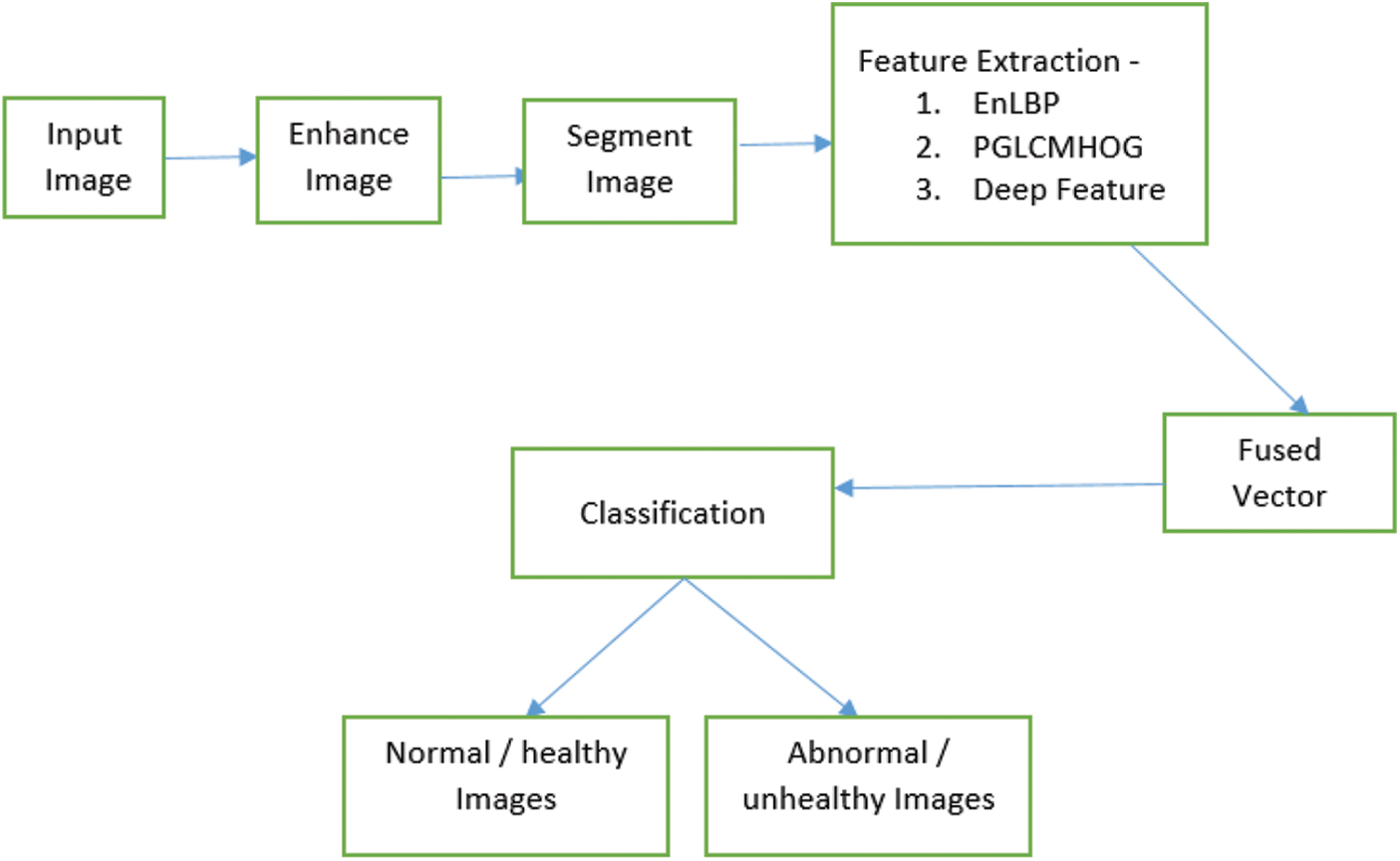
Figure 3: Workflow of the EFFS based classification method

3.1 MRI Image Pre-Processing

Being the basic step in analyzing an MR image Pre-Processing is not the easiest of all in visualization due to the occurrence of noise as well making it rigid for segregation too. Pre-processing works in three phases: Converting to Gray from the Original, neutralizing through Histogram equalization, and finally using the median filtering technique. The images are converted to gray color to shrink the complexity in analyzing the images. The image contrast is enhanced by the Histogram equalization manoeuvre [29]. The Moving Square filtering is used to moderate the undesirable qualities present in the image using smoothing while retaining the superior qualities of the image

3.1.1 Grey Conversion Using Lumosity Method

The process of converting the original MR image color code to gray-scale is done using the Lumosity mechanism over additive pixel values of varied percentages of Red, Green, and Blue. Given below is the Eq. (1) for the same. Fig. 4a presents the original MR image and Fig. 4b presents its gray counterpart.

Pgrey=((0.30∗PRed)+(0.60∗PGreen)+(0.10∗PBlue)) (1)

Figure 4: Original MRI image and its Gray version

3.1.2 Histogram Equalization Technique

The converted image contrast is improved by applying a Histogram optimization operation. In this, the intensity is spread out so the least intensity value associated with any pixel will be pushed to a higher degree. The mapping of these value changes using this equalization approach is done using PDF (Probability Density Function) approaches. The PDF approach represents the pixel strength as Ps and is set as Eq. (2):

pdfp(Si)=IiI (2)

Here in Si the i value is set between 0–255, Ii refers to the incidence of the pixel strength Si in the image, I refers to the number of pixels associated with the image. Histogram is designed with the value obtained through PDF function against pixel strength. The enhanced intensity level is provided by Eq. (3).

Ei=∑x=0iIxI (3)

The outcome after applying the new intensity level would enhance the contrast extensively. Now the image is provided to Median Filter.

3.1.3 Filtering the Image Using Median Filter

The central pixel value is updated based on the median of values associated with the pixel in a moving window. The window passes point by point in the image to capture the values of each pixel to find a new central pixel value for every slide. The moving window is provided with a non-even size that is the window size (W x W) where ‘W’ would be from {3,5,7…}. For an MRI image of the dimension (A x B), select the start point as S(x, y) such that x and y values are contained in dimension of the image. Eq. (4) deals with the above-mentioned process

K(x,y)=med{K(x+r,y+c)} (4)

where r,c belongs to (−(W−12),…(W−12)) and W(r,c) = gives intensity of point(r,c). This filter is highly looked upon for its ability to remove salt and pepper noise, thus provides smoothing with edge preserving as well. The Fig. 5 given below shows the enhanced image after removal of noise using median filtering technique.

Figure 5: Original image along with enhanced version of the MR image

3.2 IQPFLSM Segmentation Technique

A segmentation technique based on Fuzzy Level Set Method along with Improved Quantum Particle swarm Optimization technique is used to provide a better segmented image.

3.3 Deep Feature Extraction Based on Enhanced Local Binary Pattern (Enlbp) & Partisan Graylevel Co-Occurrence Matrix Histogram Oriented Gradient (PGLCMHOG)

ELBP (Enhanced Local Binary pattern) is used to get the features from the images that have been split into parts. This helps to get a new value for the middle cell based on its neighbors. Odd numbers are used to show the size of the sub-image most of the time. Center (seed) cell: The median value of the cells around it is found. If the median value is close to, or lower than the median value, the corresponding cell value is changed to 0. If it is not, the cell value is changed to 1. To make the window bigger, make sure the cell values around it are all binary digits. Make that value the new centre value of the window. Now, do the same thing for each dimension of the picture. This gives each cell a new value, which makes a feature vector in the form of cell histograms. A mid-range operation is used to make the histogram look the same across the board. All the cell histograms are combined into a single super vector. Objects can be identified in pattern recognition by their Histogram Oriented Gradient attributes. In the proposed work, the PGLCMHOG (Partisan Gray Level Co-occurrence Matrix Histogram Oriented Gradient) is used to look for attributes in images that have been segmented. These images have been preprocessed before they are segmented. A new method called Partisan-GLCMHOG is being proposed. First, the inclination of images from MR modalities is calculated. For each cell in the given segmented images, the angle of each cell in terms of both course and level has been found. The Eqs. (5) and (6) are used to figure out what course and level you are on.

Sx=Coursealongi=((i,j−1),(i,j+1)) (5)

Sy=Coursealongj=((i−1,j),(i+1,j)) (6)

where Sx & Sy forms two matrices to represent slope along horizontal and vertical course. Using these values the level is calculated using Pythagoras theorem squareofslope=squareofsumofothertwosides used to yield the level and tan⁡∂=SySx provides the course of every pixel in the image. The algorithm uses level of the specified input image to proceed further in getting the final feature vector. Eq. (7) is utilized to enhance the accuracy and also for generating the feature vector. Offsets of the co-occurrence matrix is obtained from GLCM mechanism and level of input image.

CoΔu,Δv(r,c)=∑i=1n⁡∑j=1m⁡{δ∗P(i,j),(i+Δu,j+Δv) (7)

whereδ={@lc@1ifOri(i,j)=randOri(i+Δu,j+Δv)=c0Otherwise

P(i+Δu,j+Δv),(i,j)=(Li,jZ∗Li+Δu,j+ΔvZ)+1 (8)

The Slope level of the location represented by i, j in the given MR image is represented by Li,j, the median of the slope level of the image A is given by Z. PGLCM is calculated for all the trivial sections of the prearranged image. The PGLCM for all the 8 × 8 patches are pooled as a sole vector. The offsets are the major components in identifying the native and universal features based on their nearness and farness. Deep features for segmented MR image is extracted using VGG 19 model which has max-pooling preceded by a convolutional layer and trailed by fully connected layers. Feature mapping is accomplished by expending the input MR images with that of linear filter banks for convolution. ReLU is expended in harnessing the features of the MRIs after training is completed on these MR images to learn them effectively. The network starts with 240 mappings to features from the initial convolutional layer which extends up to 4096D vector as the expected sequence, which serves as input to the softmax layer for further computation.

3.4 Synthesis of EnLBP, PGLCMHOG and Deep Features

Synthesis data is a widely accepted practice in quite a lot of applications related to computer vision and machine learning. The process of synthesis of features/attributes/properties is considered the most critical activity in image processing, which requires a careful blending of many vectors which contain information related to the feature of the MR image. The feature synthesis is done based on the entropy mechanism. The three vectors that are used for fabricating the fusion vector are given below:

AiLBP(1xg)={EnLBP1x1,EnLBP(1x2),EnLBP(1x3),……..,EnLBP(1xg) (9)

APGLCMHOG(1xh)={PGLCMHOG1x1,PGLCMHOG1x2,,……..,PGLCMHOG1xh (10)

AVGG19(1xf)={VGG191x1,VGG19(1x2),VGG19(1x3),……..,VGG19(1xf) (11)

S1xz=∑i=13⁡{Attributesof(EnLBP,PGLCMHOG,VGG19) (12)

where zε(g+h+f) . The element of ‘S’ is the fused vector fabricated by combining EnLBP is 1 × z. The features selected based on entropy are applied to EnLBP, PGLCMHOG, and VGG19 individually and the best among the aggregated features are selected based on the score of each attribute. The scores are calculated based on PCA (Principal Components Analysis). These values let the entropy-based mechanism select relevant attributes. The process is accomplished by the following formulation provided through (13) & (14) below.

Ey=−TAEyb∑i=1m⁡Prob(Ai)∗log2Prob(Ai) (13)

SC=Ey(max(Ai,Ey)) (14)

here, TA represents the overall attributes in the set and Boltzman entropy is used along with this value, in determining the best attributes to be used. The entire mechanism is mirrored in the Fig. 6 provided below. At the terminal step, the syntheszsed attributes are fed to multiple classifiers to observe and identify the effective ways in which they classify the provided input in the form of MRIs.

Figure 6: Block diagram of feature fusion

3.4.1 Dataset

The benchmark data set of BRATS 2015 [30] has 54 cases with ground truth stating 54 Low-grade glioma and 220 high-grade glioma is used which consists of Flair, T1 & T2 images. The suggested system is tested on the overtly obtainable dataset. From the data set 1/3 of it are included for training and 2/3 of the data are used for testing purposes. The image is the data are of 240 × 240 dimensions with nearly 150 slices in each case.

3.5 Classifiers

Using benchmark dataset performance of classifiers of different nature are scrutinized. The performance of each classifier is validated by looking at how accurately they differentiate the abnormal cell region from that of normal cell region visibility in the MR images. Binary classification is achieved using function like quadratic kernel along with SVM. KNN classifier is used which evaluates and classify the image based on five neighboring pixel intensity. Interdependency is the base line of classifier namely Decision Tree (DT), where a tree structure is maintained and the nodes are allotted with properties with labels. Another classifier named Random forest devised based on 100 × 2 DT are used. A classifier based on probability named Naïve Bayes along with another classifier Logistic Regression (LGR) are the few classifiers used for the classification analysis mechanism. The all-inclusive scrutiny is piloted with normal and abnormal cell MR image modalities

4  Experimental Results and Discussion

The experiment is done to be sure that the proposed system’s effects on public data can be seen clearly. First, the experiment looks at how the performance improves after the image is changed. The experiment also points out that there has been a big improvement in the use of the segmentation technique and a small change to the grab cut method of segmentation. Finally, the results of the experiments are used to see what happens when features from different techniques are combined and fused together to classify the tumor correctly. Matlab 2018b is needed for the experiment, as well as Intel core I7 3.4 GHz and NVIDIA GeForce GTX 1080 GPU. People use the most common methods to see how well things work after they’ve been improved, like Peak Signal to Noise Ratio (PSNR), Mean Square Error (MSE), and Structural Similarity Index (SSIS) (SSIM). The difference between the image from the dataset and the image from the enhanced MR image slices is found by using the MSE method. MSE with a low value helps a lot with the task of segmentation. Similarly, PSNR is used to show how much noise is in an image by giving it a low value. If PSNR is high, the image has less of an impact because of artefacts like noise. There are a lot of different ways to figure out how many pixels there are in an image. The PSNR value comes from subtracting the value of MSE from the number of pixels. The mean, variance, and contrast factors of MR images are used to get a sense of how similar the original and enhanced images are. From Eqs. (17) to (20), true, more performance measures for the segmentation mechanism can be used to evaluate how well it works.

Accuracy=Truecorrect+TrueincorrectTruecorrect+Trueincorrect+Falseincorrect+Falsecorrect (15)

SE=TruecorrectTruecorrect+Falseincorrect (16)

SP=TrueincorrectTrueincorrect+Falsecorrect (17)

DSC=2∗Truecorrect2∗Truecorrect+Falseincorrect+Falsecorrect (18)

Segmentation process is evaluated by precision and recall value which are provided in equation given below (19) and (20).

Precision=TruecorrectTruecorrect+Falseincorrect (19)

Recall=TruecorrectTruecorrect+Falsecorrect (20)

The outcome-based on all the above performance metrics is shown in Figs. 7 and 8 provided below. Figs. 7 and 8 shows the classification outcome on Brats 2015 based on (LGG & HGG) Low-Grade Glioma and High-Grade Glioma. In Tab. 1 various Enhancement fallouts matched with prevailing methods are provided to better understand the existing methodologies.

Figure 7: Consequences of defective and non-defective (Brats2015)

Figure 8: Classification outcome of LGG and HGG (Brats2015)

The evaluation is carried on the three types of features obtained namely EnLBP + PGLCMHOG, Deep features using VGG19 and Synthesized vector based on the former vectors. The outcome of classification based on all of the above is depicted in Figs. 7 and 8. The classifier Logistic Regression (LGR) showed a greater accuracy of 0.9990 in proposed mechanism, while exhibiting 0.9887 in specificity with 0.9967 sensitivity (Fig. 7). DT classifier has achieved an accuracy score as 0.999, followed by 0.9981 in specificity and 0.9957 in sensitivity. KNN showed an increased outcome in sensitivity with 0.9857 along with specificity of 0.9981, providing accuracy with 0.9954. Most widely appreciated and welcomed classifier SVM secured accuracy of 0.999 using EEFS mechanism, followed by logistic regression. specificity close to KNN with 0.9984 and sensitivity less compared to KNN with 0.9965.

The successful classification of HGG and LGG is presented in Fig. 8 expending BRATS 2015 data set. Here KNN performed well in terms of precisely classifying HGG and LGG using EFFS with 0.9052 accuracy along with sensitivity by 0.8699 and specificity 0.9052. On BRAQTS 2015 specificity obtained through SVM is accounted the highest among other classifier using EEFS with 0.9614 in terms of specificity with slightly low accuracy of 0.893 compared with KNN. The above has considerably validated the proposed EEFS mechanism and stands as a proof that the proposed is producing exceptionally well in comparison with existing methods (Fig. 7). The running time of the mechanism suggested in the work is illustrated in Fig. 9 and Tab. 2.

Figure 9: Computational comparison of EEFS with existing methods

5  Conclusion

Segmented images play a big part in making the features for classifiers. The deep features and the features based on enhanced LBP and Hog with Paristan GLCM played a big role in making a good feature vector. The most important and important features are found and fused in a sequential way to make a single-dimensional vector. The different classifiers were fed the fused data from the above process, and they were able to tell which images were normal and which were not. This is a very good result. In this case, the method used to train the system and test its performance with the BRATS 2015 dataset was used. There was the best outcome in terms of accuracy = 0.9991 and DSC = 0.9987. This is a valid point in claiming that the proposed mechanism is better than any other mechanism that is already out there. It will be possible in the future to use both the pathological report and features from images to plan a very specific treatment for a quick and accurate diagnosis, and this could be done very well.

Funding Statement: The authors received no specific funding for this study.

Conflicts of Interest: The authors declare that they have no conflicts of interest to report regarding the present study.

References

 1.  A. R. Kavitha, L. Chitra and R. Kanaga, “Brain tumor segmentation using genetic algorithm with SVM classifier,” International Journal of Advanced Research in Electrical, Electronics and Instrumentation Engineering, vol. 5, no. 3, pp. 1468–1471, 2016. [Google Scholar]

 2.  T. Logeswari and M. Karnan, “An improved implementation of brain tumor detection using segmentation based on hierarchical self organizing map,” International Journal of Computer Theory and Engineering, vol. 2, no. 4, pp. 591–604, 2010. [Google Scholar]

 3.  G. K. Khambhata and R. S. Panchal, “Multiclass classification of brain tumor in MR images,” International Journal of Innovative Research in Computer and Communication Engineering, vol. 4, no. 5, pp. 1–12, 2016. [Google Scholar]

 4.  G. Kaur and J. Rani, “MRI brain tumor segmentation methods a review,” International Journal of Computer Engineering and Technology, vol. 6, no. 3, pp. 1–10, 2016. [Google Scholar]

 5.  N. R. Bertos and M. Park, “Breast cancer-one term, many entities?,” Journal of Clinical Investigation, vol. 121, no. 6, pp. 3789–3796, 2011. [Google Scholar]

 6.  K. Komaki, N. Sano and A. Tangoku, “Problems in histological grading of malignancy and its clinical significance in patients with operable breast cancer,” Breast Cancer, vol. 13, no. 3, pp. 249–253, 2006. [Google Scholar]

 7.  N. Nida, M. Sharif, M. U. G. Khan, M. Yasmin and S. L. A. Fernandes, “A framework for automatic colorization of medical imaging,” A Journal of Multidisciplinary Science and Technology (IIOAB), vol. 7, pp. 202–209, 2016. [Google Scholar]

 8.  E. Bullmore and O. Sporns, “Complex brain networks: Graph theoretical analysis of structural and functional systems,” Nature Reviews Neuroscience, vol. 10, no. 3, pp. 186–198, 2009. [Google Scholar]

 9.  V. Rajinikanth, S. C. Satapathy, S. L. Fernandes and S. Nachiappan, “Entropy based segmentation of tumor from brain MR images–A study with teaching learning based optimization,” Pattern Recognition Letters, vol. 94, no. 1, pp. 87–95, 2017. [Google Scholar]

10. B. Mughal, M. Sharif, N. Muhammad and T. Saba, “A novel classification scheme to decline the mortality rate among women due to breast tumor,” Microscopy Research and Technique, vol. 81, no. 2, pp. 171–180, 2018. [Google Scholar]

11. G. Castellano, L. Bonilha, L. M. Li and F. Cendes, “Texture analysis of medical images,” Clinical Radiology, vol. 59, no. 12, pp. 1061–1069, 2004. [Google Scholar]

12. R. J. Gillies, P. E. Kinahan and H. Hricak, “Radiomics: Images are more than pictures, they are data,” Radiology, vol. 278, no. 2, pp. 563–577, 2016. [Google Scholar]

13. K. E. Emblem, F. G. Zoellner, B. Tennoe, B. Nedregaard, T. Nome et al., “Predictive modeling in glioma grading from MR perfusion images using support vector machines,” Magnetic Resonance in Medicine, vol. 60, no. 4, pp. 945–952, 2008. [Google Scholar]

14. N. Marshkole, B. K. Singh and A. Thoke, “Texture and shape based classification of brain tumors using linear vector quantization,” International Journal of Computer Applications in Technology, vol. 30, no. 11, pp. 21–23, 2011. [Google Scholar]

15. H. Fujita, Y. Uchiyama, T. Nakagawa, D. Fukuoka, Y. Hatanakaet et al., “Computer-aided diagnosis: The emerging of three CAD systems induced by Japanese health care needs,” Computer Methods and Programs in Biomedicine, vol. 92, no. 3, pp. 238–248, 2008. [Google Scholar]

16. K. R. Laukamp, “Fully automated detection and segmentation of meningiomas using deep learning on routine multiparametric MRI,” European Radiology, vol. 29, no. 1, pp. 124–132, 2019. [Google Scholar]

17. J. Amin, M. Sharif, M. Yasmin and S. L. Fernandes, “Big data analysis for brain tumor detection: Deep convolutional neural networks,” Future Generation Computer Systems, vol. 87, no. 8, pp. 290–297, 2018. [Google Scholar]

18. J. Amin, M. Sharif, M. Raza and M. Yasmin, “Detection of brain tumor based on features fusion and machine learning,” Journal of Ambient Intelligence and Humanized Computing, vol. 219, no. 4, pp. 1–17, 2018. [Google Scholar]

19. V. Simi and J. Joseph, “Segmentation of glioblastoma multiforme from MR images-A comprehensive review,” Egyptian Journal of Radiology and Nuclear Medicine, vol. 46, no. 4, pp. 1105–1110, 2015. [Google Scholar]

20. A. N. Arularasan, A. Suresh and K. Seerangan, “Identification and classification of best spreader in the domain of interest over the social networks,” Cluster Computing, vol. 22, no. S2, pp. 4035–4045, 2018. [Google Scholar]

21. N. Gupta and P. Khanna, “A non-invasive and adaptive CAD system to detect brain tumor from T2-weighted MRIs using customized Otsu’s thresholding with prominent features and supervised learning,” Signal Processing: Image Communication, vol. 59, pp. 18–26, 2019. [Google Scholar]

22. A. Demirhan, M. Toru and I. Guler, “Segmentation of tumor and edema along with healthy tissues of brain using wavelets and neural networks,” IEEE Journal of Biomedical and Health Informatics, vol. 19, no. 4, pp. 1–14, 2015. [Google Scholar]

23. N. Gupta and P. Khanna, “A non-invasive and adaptive CAD system to detect brain tumor from T2-weighted MRIs using customized Otsu’s thresholding with prominent features and supervised learning,” Signal Process Image Communication, vol. 59, pp. 18–26, 2017. [Google Scholar]

24. N. Nabizadeh and M. Kubat, “Brain tumors detection and segmentation in MR images: Gabor wavelet vs. statistical features,” Computer Electrical Engineering, vol. 45, no. 3, pp. 286–301, 2015. [Google Scholar]

25. P. K. Sran, G. Savita and S. Sukhwinder, “Integrating saliency with fuzzy thresholding for brain tumor extraction in MR images,” Journal of Visual Communication and Image Representation, vol. 74, no. 102, pp. 102964, 2021. [Google Scholar]

26. M. Huang, W. Yang, Y. Wu, J. Jiang, W. Abbasi et al., “Brain tumor segmentation based on local independent projection based classification,” IEEE Transactions on Biomedical Engineering, vol. 61, no. 10, pp. 2633–2645, 2014. [Google Scholar]

27. K. Kamnitsas, C. Ledig, V. F. Newcombe, J. P. Simpson, A. D. Kane et al., “Efficient multi-scale 3D CNN with fully connected CRF for accurate brain lesion segmentation,” Medical Image Analysis, vol. 36, no. 5, pp. 61–78, 2017. [Google Scholar]

28. J. Kleesiek, A. Biller, G. Urban, U. Kothe, M. Bendszus et al., “Ilastik for multi-modal brain tumor segmentation,” in Proc. MICCAI BraTS (Brain Tumor Segmentation Challenge), Boston, Massachusetts, pp. 12–17, 2014. [Google Scholar]

29. R. Radha, R. GopalaKrishnan and E. Sasikala, “A review on skull extraction process from MRI images using intelligent techniques,” International Journal of Advanced Science and Technology, vol. 29, no. 5, pp. 1–18, 2020. [Google Scholar]

30. B. H. Menze, A. Jakab, S. Bauer, K. C. Jayashree, K. Farahani et al., “The multimodal brain tumor image segmentation benchmark (BRATS),” Medical Imaging, IEEE Transactions, vol. 34, no. 10, pp. 1993–2024, 2015. [Google Scholar]