Optimal Routing with Spatial-Temporal Dependencies for Traffic Flow Control in Intelligent Transportation Systems

1  Introduction

Taxis have become one of the most popular methods of urban ITS in terms of their flexibility and convenience [1,2]. Taxis are an irreplaceable segment of the urban IDS and cater to the travel needs of an extraordinary number of people. In many cities, however, people who want to demand a taxi are accustomed to parking an empty taxi by “roadside beckoning”. As a result, the areas where taxi drivers receive their passengers are exceptionally arbitrary [3,4]. Both those who want to get a taxi and taxi drivers do not have enough data about a better area, which makes it surprising that a taxi driver experiences difficulties in locating passengers, while people think it is not easy to find an empty taxi. Empty taxis in urban street networks not only make use of unwanted energy (i.e., oil and gas) but also use the extra street space, thus making congestion of traffic and air pollution problems.

Lately, taxis have been generally outfitted with global positioning system (GPS) sensors, which are cell phones that can screen taxi areas and situations with customary stretches. Accordingly, an enormous number of GPS directions with spatial-temporal data have been gathered. A lot of tracking information gives an extraordinary chance to find certain data and comprehend taxi drivers’ driving practices, mobility of humans, and the elements of street networks [5,6]. The extraction of taxi GPS directions has gotten expanding consideration from information mining, smart transportation, development designs, and omnipresent figuring networks.

Few research works focus on strategies of the driver for locating passengers [7–10]. This will help to enhance travel efficiency and decrease unnecessary travel time by exploring the travel patterns of experienced drivers. Besides, many studies focus on finding the hot spots of pick-up spots [11,12]. Road networks have hotspots for pick-up locations at different times of the day. Experienced drivers know that the road network is more likely to drop off passengers and pick up passengers quickly instead of being empty. In this work, reduction of customer waiting time at hotspots at maximum times and controlling its traffic flow are focused on. So, to attain these goals, the following contributions are presented in this paper.

•   To find the hot spots in a particular region during peak hours, these hot spots are to be clustered. For clustering, the DBSCAN algorithm is presented. Using this algorithm, closed points are grouped andthe remaining points are kept as outliers in low-density regions.

•   Among the multiple routes between the location of the taxi and the hot spot, an optimal route is selected using Rain Optimization Algorithm and is allocated to the taxi driver.

•   The proposed approach is simulated in the platform Java.

•   The performance of the proposed scheme is analyzed in terms of total waiting time, travel time, and fuel consumption.

The remaining sections of the paper are sorted as follows. Section 2 surveys some recent literature that focused on research in ITS. Section 3 proposes ROA-based optimal routing using spatial-temporal dependencies for traffic flow control in ITS. Section 4 discusses the evaluation of the proposed schemes in terms of waiting time, travel time, and fuel consumption. The conclusion of this paper is described in Section 5.

2  Related Works

A lot of researchers had developed Traffic Flow Control in Intelligent Transportation Systems. Among them a few research works are reviewed here; Ghorai et al. [13] had presented a beaconless traffic-aware geographical routing protocol based on optimal path selection in a traffic surveillance system. This protocol considered traffic density, distance to the next forward node, and route selection for the direction and route selection process. In the old days, for the routing process, the geographical routing protocol was used due to the low overhead. Nevertheless, with many advantages, geo-routing protocols are not considered as many barriers to the vehicle environment. This approach overcame difficulties in the geographic routing protocol. This protocol is feasible for urban dense and scattered traffic conditions and faces delays, disconnections, and pocket-dropping problems.

Pourazarm et al. [14] had developed a Strength Pareto Evolutionary Algorithm (SPEA)-based multi-metric routing protocol for intelligent transportation systems. The authors aimed to increase the packet delivery ratio and reduce the delay. To attain this goal, they had presented a multi-metric routing protocol. With this protocol, the authors included the SPEA algorithm to select the path with minimum distance, delay, and maximum V2V connectivity. Using this SPEA algorithm, the five metrics such as delay, link capacity, distance, connectivity, and relative velocity were optimized and the fitness value was calculated. Then the optimal path was found if it satisfied the fitness value of the SPEA algorithm.

Abbasi et al. [15] had developed energy awareness optimal routing in the transport network. Here, they used their optimal routing scheme to a sub-network of the East Massachusetts Transportation Network utilizing real traffic data contributed by the Boston Regional Metropolitan Planning Organization. With this data, they evaluated cost functions and explore the best solutions attained under various charging stations and energy-conscious vehicle loads.

Chen et al. [16] had developed an effective parallel genetic algorithm for the problem of vehicle routing in cloud implementation of the ITS. The suggested approach significantly speeds up the resolution of the equivalent DSP of multiple complex vehicle routing problems (VRPs) in the cloud operation of ITS. The proposed scheme parallels GA by formatting three kernels simultaneously, each running some of GA’s dependent operators. It can be directly modified to run on multi-core and multi-core processors. To make better use of the valuable resources of such processors in the parallel operation of GA, the texts operating on the three kernels are synchronized by a low-cost conversion mechanism. The recommended method was tested to convert DSP’s GA-based solution in parallel in multi-core and multi-core systems.

Li et al. [17] developed Traffic flow guidance algorithm in ITS including the impact of a non-floating vehicle. Along with the estimation scheme, a novel traffic flow guidance mechanism called Estimated Weight Vehicle Density Feedback Strategy based on Weight Vehicle Density Feedback Strategy (WVDFS) was presented. In the simulation, the guiding impact of the novel algorithm was executed depending on the two-way scenario, which is a simplified model of the transport network. The Nash model was also utilized as a vehicle movement model, which can simulate vehicle movement. Simulation results depicted that floating vehicles have a major negative influence on the execution of WVDFS, and the compatibility of our algorithms is verified for optimal performance in incomplete information sequences.

Togou et al. [18] had analyzed the influence of traffic signs on pedestrian path selection behavior and developed a MAKLINK map to study the effect of traffic signs on pedestrian sequence results by a simulation technique. With the MAKLINK map, the route plan is divided under the guidance of traffic signs. Then, the optimal pedestrian path on the MAKLINK map is improved via the Ant Colony algorithm including the impact of traffic signs. The experiential study is conducted at Beijing South Railway Station. The findings reflect that traffic signs within the urban rail transport hub may be effective for the route selection behavior of a large number of passengers.

Kumari et al. [19] proposed the selection of an altruistic service channel for VANET to select the minimum congested service channels for V2 non-safety applications. Dharani & Shylaja (2019) had developed an Analytical Hierarchical Process (AHP) based geographical routing protocol for the urban environment of VANETs. In this paper, multiple routing was considered. For multiple routing, they considered link lifetime, node density, and node status. The protocol used the computed single-weighing function to find a next hop node within a defined range which can ensure an improved forwarding process.

3  ROA-Based Optimal Routing Using Spatial-Temporal Dependencies for Traffic Flow Control in ITS

3.1 Overview

As the waiting time of the customer is the main concern in ITS, the optimal route is to be allocated to the taxi driver who can reach the customer quickly. Fig. 1 shows the workflow of the proposed scheme. With the spatial-temporal dependencies, during rush hours, pick-up locations or hot spots in a region are clustered using the density-based spatial clustering algorithm. Using this algorithm, closed points are grouped and the remaining points are kept as outliers in low-density regions. After clustering, based on the demand of the customer from the particular hot spot, the optimal route is allocated to the taxi driver who can reach the hot spot quickly. Before allocating the optimal route, each route between the taxi driver and the hot spot is mapped to the number of taxi drivers. Among the map function, the optimal map is selected using the rain optimization algorithm (ROA). If more than one map function is obtained as the optimal solution, the map between the route and the taxi driver who has done the least number of trips in the day is chosen as the final solution.

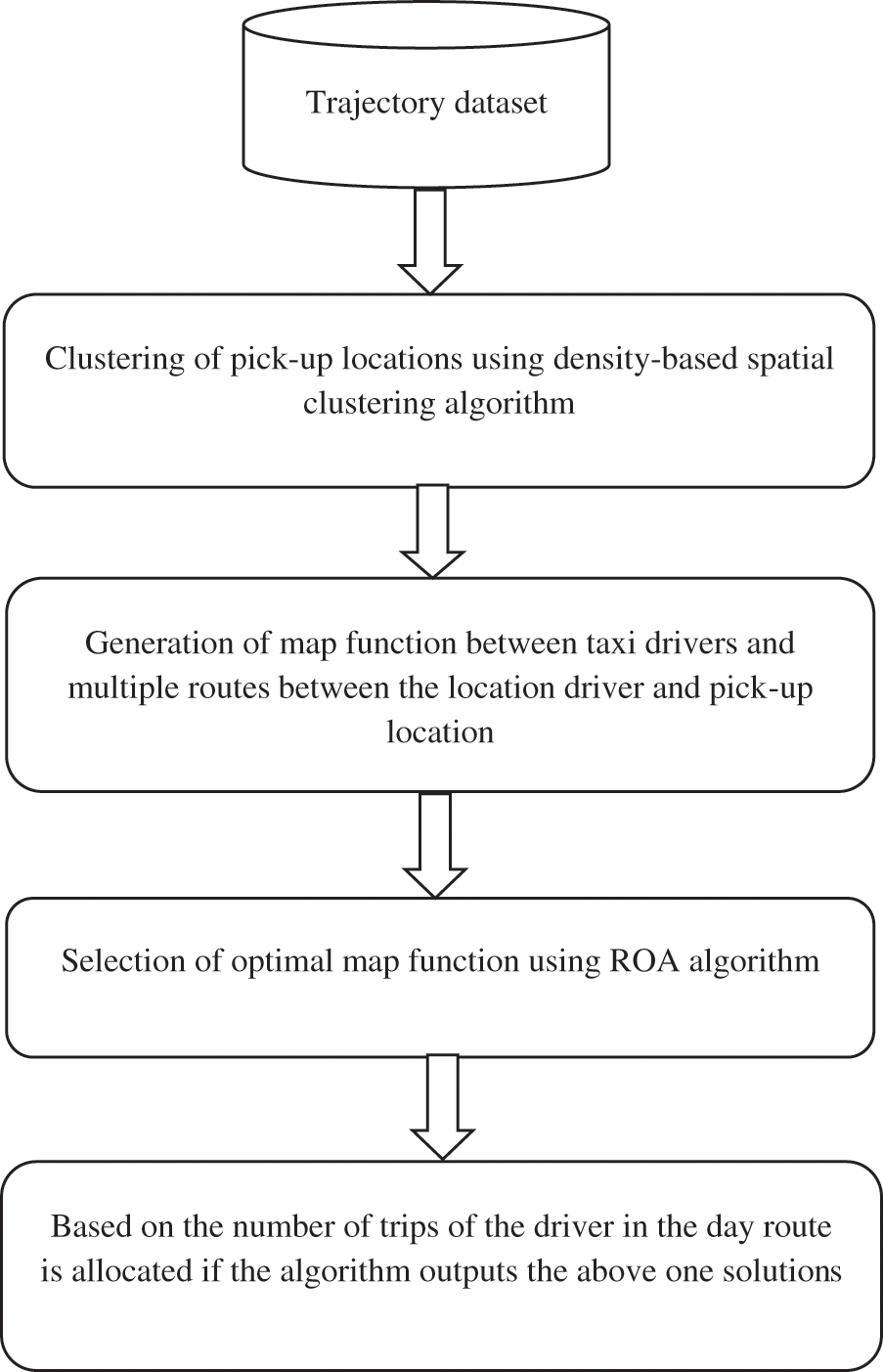
Figure 1: Workflow of the proposed scheme

3.2 Clustering of Hotpots

During the peak hours, the experienced drivers reach or wait at locations to pick up the passengers as they know well the details of pickup locations such as railway stations, bus stands, shopping centers, and so on. These pick-up locations are also known as hot spots. From these hot spots, taxi drivers may receive maximum customer demand for travel. So, in this work, from the spatial-temporal data, high-demand regions are explored using the historical pick-up information. Besides, distribution patterns of pick-up hot spots are analyzed. So, to find the hot spots during the peak hours in an urban area, clustering is the major solution.

With spatial-temporal trajectory data, hot spots in a particular region are clustered using a density-based spatial clustering algorithm at the period of rush hours. Density-based clustering can organize geographical attributes. In this approach, hot spots or pick-up locations are discovered with the DBSCAN algorithm. From the spatial-temporal dataset, this algorithm forms a group by combining the hotspots that have similarities in terms of high-density regions and low-density regions that are marked as outliers. Epsilon (Eps) and minimum points (MinPts) are major parameters used in DBSCAN for clustering.

For a given spatial-temporal dataset, DBSCAN forms arbitrary-shaped clusters. Also, it separates the noise points in the dataset. This algorithm uses a radius value (Eps(e)) which represents a user-defined distance measure and the number of minimal points (MinPts) that must happen inside Eps. Briefly, Eps denotes the distance parameter for spatial characteristics such as longitude and latitude. For calculating Eps, the formal distance metric like Minkowski, Euclidean, or Manhattan can be applied. If a region has more points than the value of MinPts, it is considered as dense. The process of the DBSCAN algorithm is described as follows:

•   This algorithm begins with the initial point k in a dataset. Then, all points within Eps i.e., density reachable form k are retrieved. Namely, the object or point k is density reachable from the point l depending on the MinPts and Eps if there is a sequence of points k1……. kn, k1 = l and kn = l likewise ki + 1 is directly density-reachable from ki depend on the MinPts and Eps, for 1≤i≤n,ki∈Dataset . Fig. 2 shows the k density reachable from l.

•   If the object k is a core object, a cluster is created. Namely, an object is represented as a core object if it has at least MinPts of other points within the radius of Eps. Fig. 3 shows the representation of the core object and border object.

•   The object k is considered as the border object if there are no points that are density reachable from k. So, if the object k is a border object, the algorithm chooses the next point of the dataset.

•   Density-based cluster (C) should satisfy the following conditions,

∀k,l : if l∈C and k is density reachable from l depending on MinPts and Eps, k∈C

•    ∀k,l∈C : k is density-connected to l depending on MinPts and Eps.

The set of points that do not belong to any cluster is considered noise. Fig. 4 shows the representation of the noise object.

The above process is continued until processing all points in the dataset.

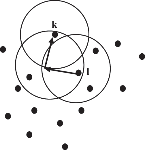
Figure 2: k density reachable from l

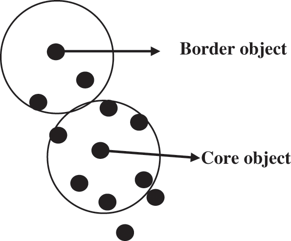
Figure 3: Core object and border object

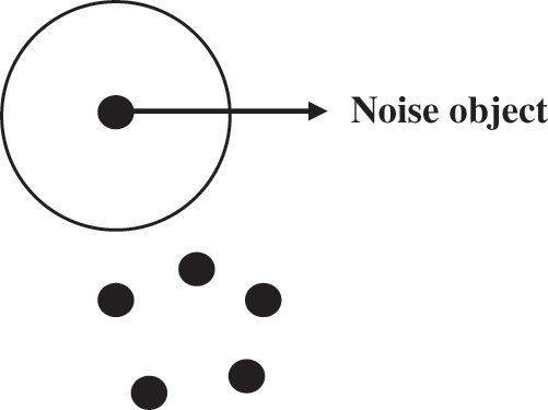
Figure 4: Noise object

So, with the spatial-temporal trajectory dataset, the DBSCAN algorithm groups the hot spots or pickup locations during peak hours. This will helps the non-experienced as well as experienced taxi drivers to identify the hot spots in a region during peak hours.

3.3 Mapping Function

After clustering the hot spots or pickup locations in the period of peak hours, routes between the hot spot and taxi drivers are estimated with the data of GPS in ITS.

Before allocating the optimal route to the taxi drivers, multiple routes are mapped with each taxi driver as shown in Fig. 5. According to the capability of the taxi and driver, the best route is determined among the multiple routes.

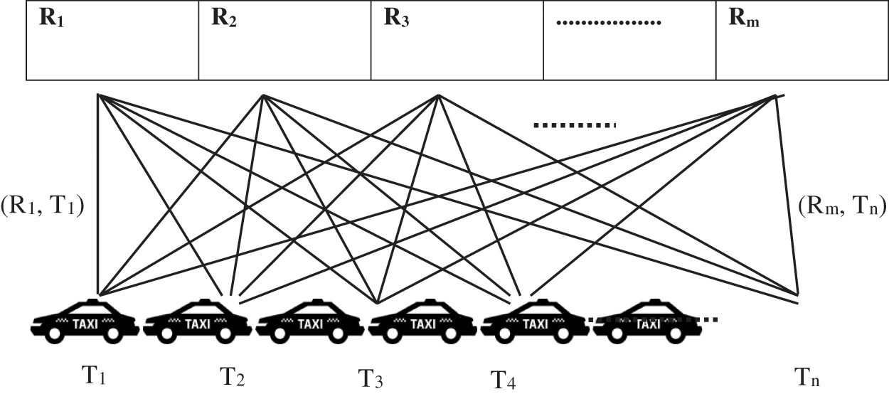
Figure 5: Mapping between taxi and routes

Finally, among the map functions, the best map function is chosen using the ROA algorithm which is explained in the section. The mathematical representation of the map function is denoted as follows,

Mn={(R1,Tn),(R2,Tn),…..,(Rm,Tn)} (1)

where, Mn denotes the mapping of multiple routes to the nth taxi or taxi driver, Rm denotes the mth route and Tn denotes the nth taxi.

3.4 Optimal Routing Using ROA Algorithm

The rain optimization algorithm (ROA) imitates the behavior of raindrops. Raindrops normally stream down along a slant from a pinnacle at that point structure the waterways and consistently move to the lowest land points or void out into the ocean. The raindrops follow breaks and overlays in the land as they stream downhill. As the water streams downhill, it may be caught in the puddles and structures of a lake known as local optimal. At last, most streams move to the ocean level known as global optimal and void out into the ocean. The manner in which the proposed strategy merges from a conjecture to the ideal is comparable to raindrops streaming from the top to the ocean level in a hilly region as per gravitation. As consistently raindrops will in general choose the way having the more extreme slant, ROA reproduces this propensity and uses the slope of the target capacity to decide the solution that is better than an estimate.

To track down the most profound valley and afterward reach the ocean level known as global optimal, a population of raindrops is created haphazardly at the initial iteration. The positions of the neighbor points of each drop are compared with the position of the drop before the drop moves towards the neighbor point possessing the least position. This development proceeds until the drop arrives at the valley. However long every one of the drops is streaming down from an upper to a lower position, regardless of whether there are puddles on the drops “route to the valley, they can in any case flood and rise out of the puddles to continue to move towards the valley by a fitting component carried out by the ROA algorithm.

The process for selecting the optimal map function using the ROA algorithm is described as follows:

Initialization: In this algorithm, each particle or raindrop in a population denotes the solution. The solution of this approach is the optimal map function. The initialization of ith drop is defined as follows,

Di={yi,1,yi,2,yi,3,…..,⁡yi,j}i∈[1,2,3,…..,s] (2)

where, s represents the size of the population, j denotes the number of optimization variables, and yi,j denotes the variables of the optimization problem. For this work, the variable can be defined as follows,

yi,j={Mn}i,j (3)

yi,j={(R1,Tn),(R2,Tn),…..,(Rm,Tn)}i,j (4)

where, Mn denotes the mapping of multiple routes to the nth tax.

Rainfall manages raindrops during the process of optimization. It is created by a uniform random distribution function and subject to every one of the constraints in Eq. (5)

yi,j=U(upj,lowj) (5)

where, U denotes the uniform distribution function, upj and lowj denote the upper and lower limits of yj.

Fitness calculation: For each initialized solution, fitness or objective function is estimated to evaluate the solution. To select the optimal map function, the map function is to be evaluated with the following fitness function,

Fiti=Min(waiting time (i)) (6)

Update the solution: As the raindrop (D) is defined as a point in N-dimensional space, the domain which has the radius vector (r) placed around the point is known as the neighborhood. The neighborhood can be updated when changes occur in the value of raindrops.

During the process of optimization, a point in the neighborhood of drop can be generated randomly. The ith drop’s neighborhood point q is denoted as NPqi. Using the following condition, the neighbor point of the drop is generated.

i=1,2,3,….,s‖u^p∗ (Di−NPqi)‖≤‖u^p∗ r‖forq=1,2,3,….,npp=1,2,3,….,z (7)

where, np denotes the number of neighbor points, ûp denotes the unit vector of the pth dimension. r denotes the size of the neighborhood in terms of a real positive vector and can be defined as follows,

r=f(itr)∗rinitial (8)

where, rinitial denotes the initial size of the neighborhood and f(itr) is denoted as a function used to adapt the size of the neighborhood within iterations.

Dominant drop: The dominant neighbor point ( NPdi ) is one of the points chosen from the drop’s (Di) neighbor point. It should satisfy the following condition,

Fit(Di)>Fit(NPdi)

Fit(NPqi)>Fit(NPdi)

Active drop: The drop is considered an active drop if it has a dominant neighbor point.

Inactive drop: The drop is considered an inactive drop if it doesn’t have a dominant neighbor point.

Process of explosion: If the drop has no sufficient neighbor points or it couldn’t continue the search process to attain the optimal minimum, the explosion process is initiated to solve this condition of the drop. Using Eq. (9), the number of neighbor points can be created in this explosion process.

npE=be×np×ce (9)

where, npE denotes the number of neighbor points created in the process of an explosion, np denotes the number of neighbor points without the process of explosion and ce denotes the counter of explosion.

The rank of raindrop: For each raindrop, rank (R) is calculated using (12) in every iteration. This rank is used in the merit order list.

V1ti=Fit(Di)|attthiteration−Fit(Di)|atfirstiteration (10)

V2ti=Fit(Di)|attthiteration (11)

Rti=order(V1ti)∗ϕ1+order(V2ti)∗ϕ2 (12)

where, V1ti denotes the difference between the fitness function of drop Di at first iteration and tth iteration, V2ti denotes the fitness function of drop Di at tth iteration, order(V1ti) and order(V2ti) denote the orders of V1 and V2 at tth iteration when they are arranged in the form of ascending order, ϕ1 and ϕ2 denote the weighting coefficients that are assumed as 0.5 and Rti denotes the rank of raindrop at tth iteration.

List of merit order: For every iteration, the ranks of the raindrops are arranged in ascending order. From the list, each low-ranking drop can be removed and some drops can be given significant rights. The drop with minimum fitness function is considered the optimal solution or map function.

Termination: The above process is repeated until getting the solution with the minimum fitness function. Otherwise, the algorithm is terminated.

3.5 Decision Phase

Using the ROA algorithm, optimal mapping of the route and taxi is attained. Then the selected taxi driver will reach the hotspot through the selected route. However, there is a possibility may occur when the optimal mapping function is being selected that the algorithm may select the one above the mapping function as the optimal solution. Namely, the algorithm may select three optimal mapping functions i.e., three taxis and three routes. At this time, the ITS system will decide to choose the taxi driver who only can reach the particular hot spot. Based on the number of travels that the taxi driver completed in a day, the taxi driver and the mapped route will be allocated. If a taxi driver has completed fewer number travels per day compared to the other two taxi drivers, then he/she will be assigned to reach the hot spot through him/her mapped route.

4  Results and Discussion

The proposed traffic flow scheme is simulated in the simulation tool of Java with the system operating system of windows 2007 with 64-bit and with 4 GB main memory at 2 GHz dual-core PC. For this work, New York City Taxi (TaxiNYC) Trip Duration dataset is used. This dataset has 1458644 trip records as a training set and 625134 trip records as a testing set. In this dataset, pickup locations are clustered using the DBSCAN algorithm.

To prove the effectiveness of the proposed approach, it is compared with other approaches. In this paper, for clustering, the DBSCAN algorithm is utilized. Besides, the optimal route selection process ROA algorithm is utilized. The experimental results were carried out based on two stages. The experimental results are listed below;

4.1 Performance Analysis Based on Clustering Algorithm

In this section, the effectiveness of the proposed clustering is analyzed. In routing, clustering is an important stage. The clustering process mainly reduces the time and computation complexity. In this section, the work is compared with and without clustering algorithm-based routing.

In Fig. 6, the performance of the proposed approach is analyzed in terms of waiting time for varying numbers of vehicles. When analyzing Fig. 6, our proposed approach attained the minimum waiting time of 2.45787 s which is 3.56897 s for without clustering-based traffic flow control in intelligent transportation systems. As per the analysis, the number of vehicles increases; the waiting time also gradually increases. From the results, it’s clear that the clustering algorithm is most important to reduce the waiting time and avoid traffic. In Fig. 7, the performance of the proposed approach is analyzed in terms of traveling time by a varying number of vehicles. Traveling time is measured based on how much time is taken to reach the destination. The good system has taken minimum time for traveling. When analyzing Fig. 7, the proposed approach is taken 768 s to reach the destination which is 874 s without clustering-based reach the destination. From the results, it’s clear that the proposed approach reaches the destination quickly compared to other approaches.

Figure 6: Performance analysis based on waiting time

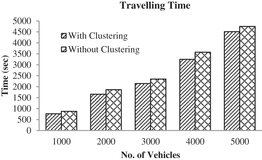
Figure 7: Performance analysis based on traveling time

The performance of the proposed approach is analyzed based on fuel emissions as given in Fig. 8. The process of path selection has a vital role in decreasing fuel emissions. The fuel emissions may be enhanced by permitting longer waiting, or starting after the rush hour. The main objective of this paper is to solve the vehicle routing problem and minimize fuel emissions. When analyzing Fig. 8, the proposed approach is taken with minimum fuel emission compared to other algorithms. In Fig. 9, the performance of the proposed approach is analyzed in terms of fuel consumption. As per the analysis, the proposed approach consumes less amount of fuel compared to other algorithms. By allowing long waiting times at customer nodes, vehicles can avoid being caught in congestion, and fuel emissions can be reduced.

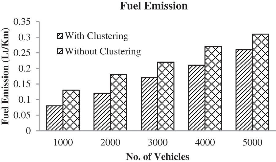
Figure 8: Performance analysis based on fuel emission

Figure 9: Performance analysis based on fuel consumption

4.1.1 Performance Analysis Based on A Route Selection Algorithm

The path selection process plays a more significant role in reducing fuel emissions and traveling time. In this paper, for the route selection process, the ROA algorithm is used. To prove the effectiveness of the proposed ROA, the algorithm was compared with different methods such as GA-based route selection, PSO-based route, and optimization-based traveling.

In Fig. 10, the performance proposed against the existing optimal path selection algorithm is analyzed in terms of waiting time. When analyzing Fig. 10, our proposed approach takes a minimum waiting time of 1.857 s for 1000 vehicles on the road which is 3.6658 s for PSO-based optimal route selection, 6.3225 s for GA-based optimal route selection on-road, and 8.456 s for without optimization based optimal route selection. This is due to ROA-based rote selection. In Fig. 11, the performance of the proposed approach is analyzed in terms of traveling time. As per the analysis, the number of vehicles increases, and traveling time also increases. The good optimal route selection algorithm reaches the destination quickly and also it takes minimum traveling time. When analyzing Fig. 11, the proposed approach takes a minimum traveling time of 745 s which is 812 s for PSO-based optimal route selection on road, 889 s for GA-based optimal route selection on road, and 956 s for without optimization-based routing. Compared to the other three algorithms, the route selection approach without optimization takes maximum time. Because this method is select the path based on the driver’s knowledge not optimally. The performance of the proposed approach is analyzed based on fuel emission as given in Fig. 12. Fuel is one of the major products for running the vehicle. The major objective of route selection is to minimize time and fuel emissions. During the traveling period, if the fuel discharge is kept to a minimum, the cost of purchasing fuel for the driver will be reduced. When analyzing Fig. 12, the proposed approach is taken a minimum fuel emission of 0.08 Lt/Km which is low compared to another algorithm. From the result, it’s clear that the proposed approach is taken minimum fuel emission compared to other methods. Similarly, a comparative analysis based on fuel consumption is given in Fig. 13. When analyzing Fig. 13, our proposed approach consumes a minimum amount of fuel of 1.14 Lt/Km which is low compared to the existing algorithm. From the results, it’s clear that the proposed approach is better than all the other algorithms.

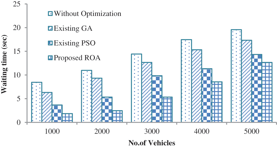
Figure 10: Comparative analysis based on waiting time

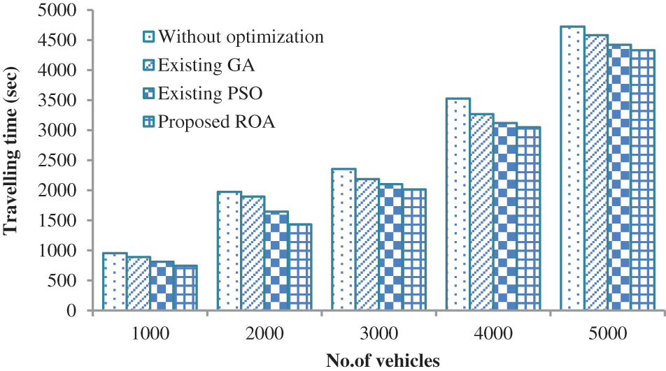
Figure 11: Comparative analysis based on traveling time

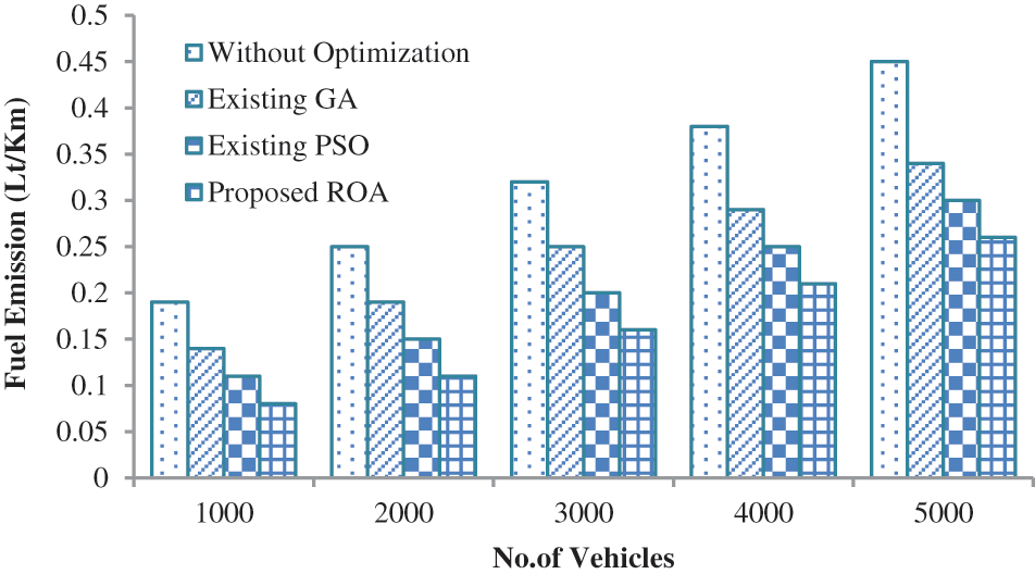
Figure 12: Comparative analysis based on Fuel Emission

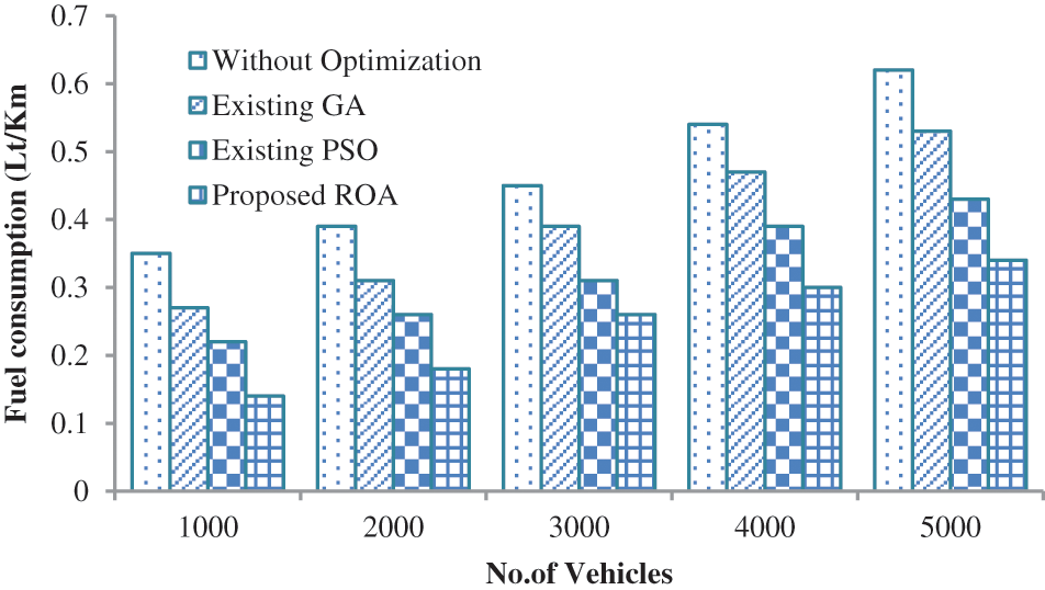
Figure 13: Comparative analysis based on fuel consumption

5  Conclusion

For traffic flow control, rain optimization algorithm (ROA) based optimal routing has been presented with the spatial-temporal dependencies. Hotspots in a region are found at the peak hours by clustering them using the density-based spatial clustering of applications with noise (DBSCAN) algorithm. After clustering, the taxi drivers reach the hotspot through the optimal route. This optimal route has been selected using the ROA algorithm. The performance of the optimal route selection based on ROA has been compared with that of the conventional algorithms GA, PSO, and without optimization algorithm. Simulation results showed that the proposed traffic flow control scheme has reduced traveling time, waiting for time, fuel consumption, and fuel emissions.

Acknowledgement: The authors with a deep sense of gratitude would thank the supervisor for his guidance and constant support rendered during this research.

Funding Statement: The authors received no specific funding for this study.

Conflicts of Interest: The authors declare that they have no conflicts of interest to report regarding the present study.

References

 1.  Y. Liu, “Big data technology and its analysis of application in urban intelligent transportation system,” in 2018 Int. Conf. on Intelligent Transportation, Big Data & Smart City (ICITBS), Xiamen, China, IEEE, pp. 17–19, 2018. [Google Scholar]

 2.  L. Zhu, F. R. Yu, Y. Wang, B. Ning and T. Tang, “Big data analytics in intelligent transportation systems: A survey,” IEEE Transactions on Intelligent Transportation Systems, vol. 20, no. 1, pp. 383–398, 2018. [Google Scholar]

 3.  L. Liqun, W. Chaozhong, Z. Hui, A. N. Hasan, C. Wenhui et al., “Research on taxi drivers’ passenger hotspot selecting patterns based on GPS data: A case study in Wuhan,” in 2017 4th Int. Conf. on Transportation Information and Safety (ICTIS), Banff, AB, Canada, IEEE, pp. 432–441, 2017. [Google Scholar]

 4.  M. G. Demissie, L. Kattan, S. Phithakkitnukoon, G. H. de Almeida Correia, M. Veloso et al., “Modeling location choice of taxi drivers for passenger pickup using GPS data,” IEEE Intelligent Transportation Systems Magazine, vol. 13, no. 1, pp. 70–90, 2020. [Google Scholar]

 5.  Y. Bo, H. Yehua and M. Xinjun, “On intelligent transportation system based on GPS and data mining,” in 2008 27th Chinese Control Conf., Kunming, China, IEEE, pp. 595–599, 2008. [Google Scholar]

 6.  M. M. Harsha and R. H. Mulangi, “Public transit travel time analysis using GPS data: A case study of Mysore ITS,” in 2018 3rd Int. Conf. on Communication and Electronics Systems (ICCES), Coimbatore, India, IEEE, pp. 407–411, 2018. [Google Scholar]

 7.  S. Liu, S. Wang, C. Liu and R. Krishnan, “Understanding taxi drivers’ routing choices from spatial and social traces,” Frontiers of Computer Science, vol. 9, no. 2, pp. 200–209, 2015. [Google Scholar]

 8.  L. Liu, C. Andris and C. Ratti, “Uncovering cabdrivers’ behavior patterns from their digital traces,” Computers, Environment and Urban Systems, vol. 34, no. 6, pp. 541–548, 2010. [Google Scholar]

 9.  X. Hu, S. An and J. Wang, “Exploring urban taxi drivers’ activity distribution based on GPS data,” Mathematical Problems in Engineering, vol. 2014, pp. 1–13, 2014. [Google Scholar]

10. D. Zhang, L. Sun, B. Li, C. Chen, G. Pan et al., “Understanding taxi service strategies from taxi GPS traces,” IEEE Transactions on Intelligent Transportation Systems, vol. 16, no. 1, pp. 123–135, 2014. [Google Scholar]

11. Y. Yue, Y. Zhuang, Q. Li and Q. Mao, “Mining time-dependent attractive areas and movement patterns from taxi trajectory data,” in 2009 17th Int. Conf. on Geoinformatics, Fairfax, VA, IEEE, pp. 1–6, 2009. [Google Scholar]

12. S. Din, K. N. Qureshi, M. S. Afsar, J. J. Rodrigues, A. Ahmad et al., “Beaconless traffic-aware geographical routing protocol for intelligent transportation system,” IEEE Access, vol. 8, pp. 187671–187686, 2020. [Google Scholar]

13. C. Ghorai, S. Shakhari and I. Banerjee, “A SPEA-based multimetric routing protocol for intelligent transportation systems,” IEEE Transactions on Intelligent Transportation Systems, vol. 22, no. 11, pp. 6737–6747, 2020. [Google Scholar]

14. S. Pourazarm and C. G. Cassandras, “Optimal routing of energy-aware vehicles in transportation networks with inhomogeneous charging nodes,” IEEE Transactions on Intelligent Transportation Systems, vol. 19, no. 8, pp. 2515–2527, 2017. [Google Scholar]

15. M. Abbasi, M. Rafiee, M. R. Khosravi, A. Jolfaei, V. G. Menon et al., “An efficient parallel genetic algorithm solution for vehicle routing problem in cloud implementation of the intelligent transportation systems,” Journal of Cloud Computing, vol. 9, no. 1, pp. 1–14, 2020. [Google Scholar]

16. Y. F. Chen, Z. Gao, H. Zhou, Y. Wang, T. Zhang et al., “Traffic flow guidance algorithm in intelligent transportation systems considering the effect of non-floating vehicle,” Soft Computing, vol. 23, no. 19, pp. 9097–9110, 2019. [Google Scholar]

17. Z. Li and W. A. Xu, “Path decision modelling for passengers in the urban rail transit hub under the guidance of traffic signs,” Journal of Ambient Intelligence and Humanized Computing, vol. 10, no. 1, pp. 365–372, 2019. [Google Scholar]

18. M. A. Togou, L. Khoukhi and A. Hafid, “Performance analysis and enhancement of wave for v2v non-safety applications,” IEEE Transactions on Intelligent Transportation Systems, vol. 19, no. 8, pp. 2603–2614, 2017. [Google Scholar]

19. N. D. Kumari and B. S. Shylaja, “AMGRP: AHP-based multimetric geographical routing protocol for urban environment of VANETs,” Journal of King Saud University-Computer and Information Sciences, vol. 31, no. 1, pp. 72–81, 2019. [Google Scholar]