INS-GNSS Integrated Navigation Algorithm Based on TransGAN

1  Introduction

With the rapid development of autopilot and aerospace technology, the precision of navigation and positioning becomes higher and higher, and the error has increased from meter level to centimeter level. In the existing solutions, GNSS and INS integrated navigation are mostly utilized to obtain high-precision navigation position information [1]. Among them, GNSS is able to provide high-precision three-dimensional position and velocity information, and the accuracy can reach centimeter level requirements [2]. Nonetheless, its performance depends on the external environment and the visibility of satellites. In terms of high mobility, tunnels and other environmental conditions, there are some problems such as low update rate and signal interruption, which seriously affect its navigation and positioning accuracy, whereas INS is an autonomous system. By continuously integrating the real angular velocity and specific force measured by the gyroscopes and accelerometers, the position, velocity and azimuth information can be obtained [3,4]. However, INS gyro drift error and accelerometer deviation will increase with time [5]. The combination of INS and GNSS (hereinafter referred to as INS-GNSS) can make up for the deficiency of INS and GNSS and lead to the improvement of the accuracy of navigation system. In INS-GNSS, Kalman filter (KF) is widely used due to its practicability [6]. When the GNSS interruption causes a severe degradation in positioning accuracy, INS-GNSS switches to pure INS mode to continue navigation. Nevertheless, due to the accumulation of navigation data errors, the positioning accuracy of pure INS will gradually decrease with time, and the performance of INS-GNSS will therefore decline during GNSS interruption [7].

Since GNSS and INS have good complementary advantages, GNSS/INS combination, known as “golden combination” in the industry, can improve the overall navigation performance and navigation accuracy of the system [8]. It mainly has the following advantages. Firstly, it can estimate and correct the error of the inertial navigation system, and improve the precision of integrated navigation; Secondly, it can make up for the defects of satellite navigation signals and improve the capability of integrated navigation; Thirdly, it can improve the capabilities of satellite navigation receiver to capture and track satellite signals, and enhance the overall navigation efficiency; Fourthly, it can increase the redundancy of observation information, and accordingly improve the monitoring ability of abnormal errors and the system fault tolerance; Finally, it can improve the anti-interference ability of navigation system and enhance the integrity of integrated navigation.

However, it is quite difficult to ensure the navigation accuracy and reliability of INS/GNSS integrated navigation system owing to the decline in the accuracy of GNSS measurement information and quality evaluation, and the impact of environmental vibration on micro inertial devices in complex and high-dynamic environment [9]. Therefore, how to improve the adaptability and robustness of MEMS-INS/GNSS integrated navigation system in complex and high-dynamic environment has become the key technology of precise guidance [10].

Common integrated navigation information fusion technologies include KF, H filter, neural network technology, etc [11,12]. Among them, there are KF and extended KF, adaptive KF, unscented KF (UKF), adaptive UKF, federated KF, particle filter, etc., which are developed on the basis of KF, and are most widely used. KF is applicable to linear system model [13], and extended KF is suitable for nonlinear system model. Among them, a variety of adaptive KF use the observed data for recursive filtering, and at the same time constantly estimate and correct the imprecise parameters and noise covariance matrix in the model [14,15], thus reducing the model errors, restraining the filtering divergence, and improving the system accuracy.

The filtering mechanism of neural network technology is to take multiple measured values as input sample values, obtain the error state estimation of the system through neural network, and then realize the feedback control of the system using the “separation theorem”, so as to quickly compensate the system errors and improve the real-time performance of the system [16,17]. It is featured by real-time data processing, parallel computing and high speed, having no specific requirements for the model structure and statistical characteristics of the integrated navigation system [18]. However, it requires a high level of neural network model. Artificial intelligence (AI) mechanism based on artificial neural network (ANN) structure can effectively improve the performance of INS-GNSS, and make INS-GNSS still obtain continuous and reliable navigation information even when GNSS is interrupted. When GNSS works normally, ANN is trained to assist INS-GNSS by adjusting the connection weights between neurons and the position or speed error of INS. Besides, the trained ANN can compensate the data errors of pure INS when GNSS interruption occurs [19]. In recent years, researchers have displayed considerable interest in transformers and made many breakthroughs. Transformer may become a powerful universal model of AI (such as classification, detection and segmentation). At the beginning of 2021, the team from the University of Texas at Austin introduced the idea of building a generative alternative network by pure transformer and achieved good results in common benchmarks such as Cifar-10, STL-10 and CelebA (64 × 64). Currently, different researchers have made great progress in all directions using transformer. Recently, (Transformer Generative Adversarial Network (TransGAN)) team updated their results, showing that TransGAN not only surpassed StyleGAN in low-resolution image tasks, but also achieved excellent results in higher-resolution (such as 256 × 256) image generation tasks [20,21]. These researches on the application of AI technology in the field of integrated navigation are relevant to the final application scenario of this paper. Moreover, some AI technologies in recent years involve various kinds of input sensor data and navigation results [22,23].

For the purpose of improving the precision of INS-GNSS integrated navigation, an INS-GNSS integrated navigation algorithm based on TransGAN is proposed, which generates a countermeasure network to compensate INS, which corrects the speed and position data during GNSS interruption, and afterwards establishes INS-GNSS aided by neural network. As the selection of neural network type has an important impact on the positioning accuracy of neural-network-assisted INS-GNSS, this paper proposes a Transformer Generic Adversary Network (TransformGAN) algorithm, which adopts multi-scale prediction to design the network structure, and adds a Transformer coding layer to the GAN network, so as to introduce global forward and backward navigation position information. The Transformer encoder is applied to generate the estimation of missing GNSS, as well as combining with countermeasure training to improve the accuracy of generating the estimation; In the process of model training, the real GNSS data is added to the GAN model as a conditional variable to better control the generation of predictive values in the model, make the generated predictive values as close as possible to the real GNSS data, and further reduce the combination error. Consequently, through the experimental analysis and comparison with MLP, WNN and KF, it is verified that this method can significantly contribute to the improvement of integrated navigation accuracy, and better restrain the influence of prediction gross error on positioning accuracy and stability.

2  TransGAN Structure

2.1 Attention Mechanism

Attention mechanism is a method of vector information fusion, which obtains the weight between vectors on the basis of the similarity between vectors. Dzmitry Bahdanau et al. proposed in 2015 that a single-layer feedforward neural network could be used in machine translation tasks to learn the positional alignment relationship between characters in the source language and the target language [24]. Based on the bidirectional LSTM network, this translation model assumes that the length of the input characters of the original language is N. and that the context vector at position i is recorded as ci in the process of decoding the characters of the target language, which is the weighted sum of the encoder vectors, as shown in Eq. (1).

ci=∑j=1N⁡αijhj  (1)

The weight between the decoded position i and the encoded position T is denoted as αij , and the entire weight matrix is expressed as A∈R(N,M) [25]. In this process, the softmax function is utilized to ensure that the sum of column edge probabilities of A is 1, as shown in Eq. (2).

αij=exp⁡(eij)∑k=1N⁡exp⁡(eik) (2)

Among them,

eij=a(si−1,hj) (3)

and

a(si−1,hj) functions learn the alignment between input and output positions. Thus, the “attention” of the decoding target character decoder focuses on the original language characters most relevant to the current position, rather than all the original language characters. The use of attention mechanism could alleviate the challenge of overlong texts in text translation.

2.2 Transformer Model

Transformer is an encoder-decoder structure. The encoder is partly stacked by stacking an input embedded layer and multiple encoder layers. The input embedding layer is responsible for maintaining three vector tables, looking up the code tables and converting them into vector representation [26]. These three vector tables consider three input conversions, namely, token index, position index, and token type index. The token index contains all the characters in the entire vocabulary. The size of the vocabulary is marked as |V| , the size of the vector table is represented by |V|×D , the position index indicates the position information of the current character in the sentence, and the size of the vector table is L×D . The size of L in this vector table determines the length of the longest string that can be processed by the converter, and the positions of characters are counted from 0 to L. The token type index, being 0 or 1, is used to distinguish two sentences that are simultaneously input into the embedded layer. It is used for tasks such as natural language inference [27]. The vector table is essentially a tensor requiring derivative, and its parameters are updated through gradient back propagation.

Each encoder layer contains a multi-head attention layer and a feed-forward layer, between which a residual connection forms. The multi-head attention layer and the feed forward neural network layer are followed by layer normalization to ensure the stability of the output value of each layer. Eq. (4) is the calculation method of layer normalization. The input normalized sample representation vector is x; Mean(X) and Var(X) are the mean and standard deviation functions; γ and β are two learnable parameters of numerical scaling; ε is a minimal parameter to prevent the denominator from being 0. Due to the existence of layer normalization, the normalized representation vector/value is not too large or too small, thus alleviating the gradient disappearance and dispersion in the training process.

Norm(X)=X−Mean(X)Var(X)+ϵ∗γ+β (4)

Eqs. (5) and (6) reflect the residual connection modes of encoder layer.

X′=X+Norm1(self−Attention(X)) (5)

X′′=X′+Norm2(Feed−forward(X′)) (6)

The representation vector shape of the input and output of each encoder layer is (n×d) , and the output vector of the last encoder layer is taken as the output vector of the encoder as a whole, which is recorded as Hencoder. The transformer encoder is shown in Fig. 1.

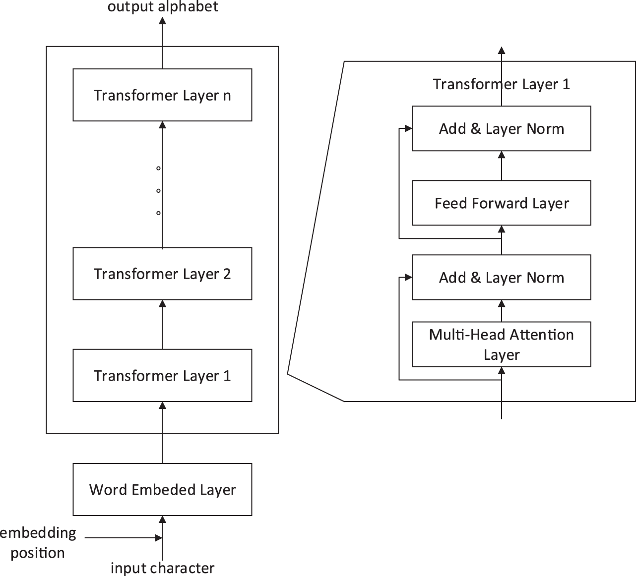
Figure 1: Transformer encoder

The decoder is formed by stacking a plurality of decoder layers. Different from the encoder layer, a cross-attention layer is added to each decoder layer to fuse the information from the encoder. If the representation vector of cross-attention layer is x, then cross-attention, (X, Hencoder) - multi-head (x, Hencoder, Hencoder). Eqs. (7)–(9) reflect the residual connection modes of the decoder layer.

X′=X+Norm1(Self−Attention(X)) (7)

X′′=X′+Norm2(Cross−Attention(X′,Hencoder)) (8)

X′′′=X′′+Norm3(Feed−forward (X′′)) (9)

The output vector of the last decoder layer is taken as the output vector Hdecoder of the decoder as a whole. The decoder is mostly used for text generation tasks. To convert the hidden vectors into token indexes, a linear transformation needs to be added as the output layer. The output layer converts the hidden vector with dimension d into Logits vector representing the decoding probability of each word. The dimension of the vector is the same as that of the vocabulary |V| .

2.3 Generating Countermeasure Network

As the most widely used model of depth image generation, generating countermeasure (GAN) was first proposed by Ian Goodfellow in 2014. The model consists of generator (G) and discriminator (D) [28,29].

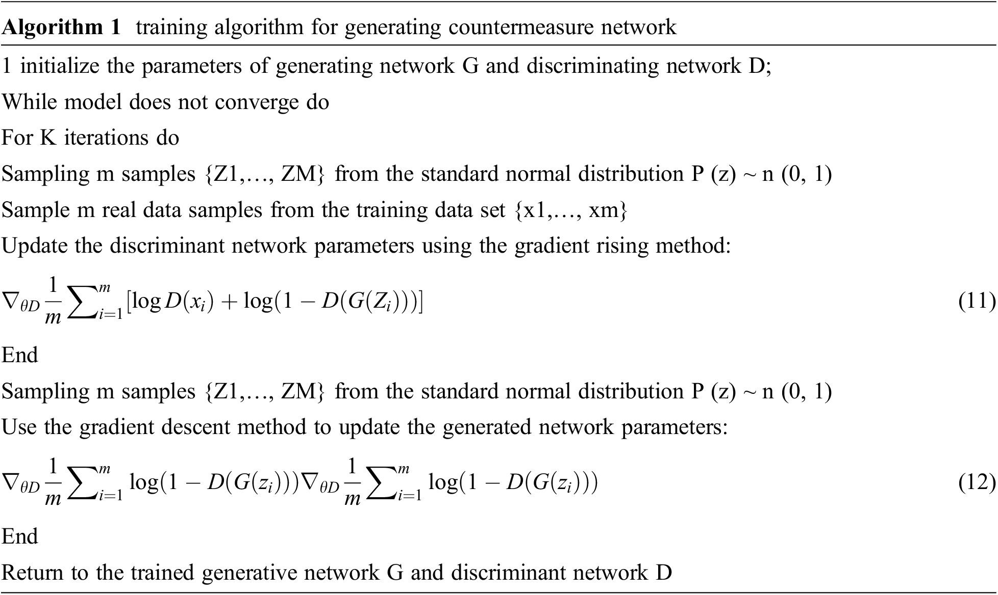
Inspired by the zero-sum game, the training process of the model is designed as a confrontation and game between the generation network G and the discrimination network D. The overall model structure diagram of the generation countermeasure network is shown in Fig. 2. The generation network G takes the random noise vector Z obeying the standard normal distribution n (0, I) as its input, and outputs the generated data g (z). The generation network attempts to generate data that makes the discrimination network indistinguishable during the training process. For the discrimination network D, in the process of training, it acts as a binary classification network, which is applied to distinguish the real training data x from the generated data g (z). In this way, the two networks are constantly engaged in confrontation training, and the two networks are optimized in mutual confrontation. After optimization, the confrontation continues. The generated data obtained by the generated network G is becoming more and more perfect, approaching the real data constantly. The specific training process of generating countermeasure network is shown in algorithm 1. In general, the discrimination network will assign the label “1” to the real data and the label “0” to the generated data. The generation network tries to make the data generated by the authentication network “misjudge” as “1”. Assuming that PR only represents the data distribution of the real data x, PZ represents the data distribution of generated data g (z), and PZ represents the prior distribution n (0, I) of the random noise vector Z. The generation network and the discrimination network are respectively represented by G and D, where D can be regarded as two classifiers. Using the cross entropy loss function, the optimization objective of generating the countermeasure network can be written in Eq. (10):

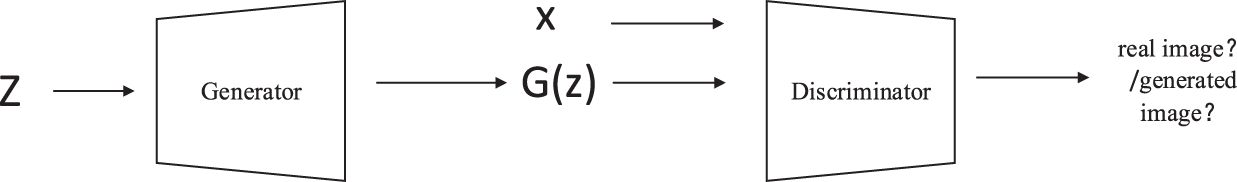
Figure 2: Schematic diagram of model structure for generating countermeasure network

minG⁡maxD⁡V(G,D)=Ex∼Pr[log⁡D(x)]+Ez∼Pr[log⁡(1−D(G(z)))] (10)

The generation countermeasure network alternately optimizes the generation network G and the discrimination network D through such a maximum-minimum game until they reach the Nash equilibrium point. Synchronously, Ian Goodfellow also proved that with the progress of alternative optimization, the discrimination network D will gradually approach the optimal discriminator. When this approximation reaches a certain degree, the optimization objective of generating the countermeasure network corresponding to Eq. (10) is approximately equivalent to minimizing the JS divergence between data distribution PR of real data and the data distribution PG of generated data (Jensen Shannon divergence). In other words, the idea of generating confrontation networks starts from the zero-sum game heuristic in game theory, which is equivalent to the optimization of the distribution distance between real data and generated data.

From the point of view of GAN model training only, as shown in Fig. 3, D plays the role of two classifiers during the training process. Each update of it enhances its ability to distinguish the real image and the generated image (i.e., correctly allocate the labels for the two kinds of data), that is, divide the correct decision boundary between the two kinds of data [30,31]. The update of G attempts to make the generated data also belong to the real data, so that the new generated data is closer to the decision boundary and real data. With the continuous process of alternating iterations, the generated data will constantly approach the real data, and ultimately make it difficult to distinguish the D, so that the generated network can fit the real data with a high degree of authenticity [32].

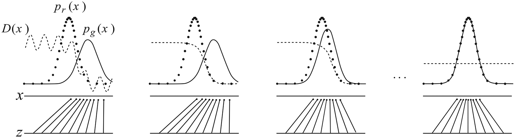
Figure 3: Changes of decision boundary and data distribution in the process of generating countermeasure network training

2.4 TransGAN Model

Yifan et al. proposed the first transformer-based GAN, which does not use any CNN or RNN structure, and is called TransGAN. The model structure is shown in Fig. 4.

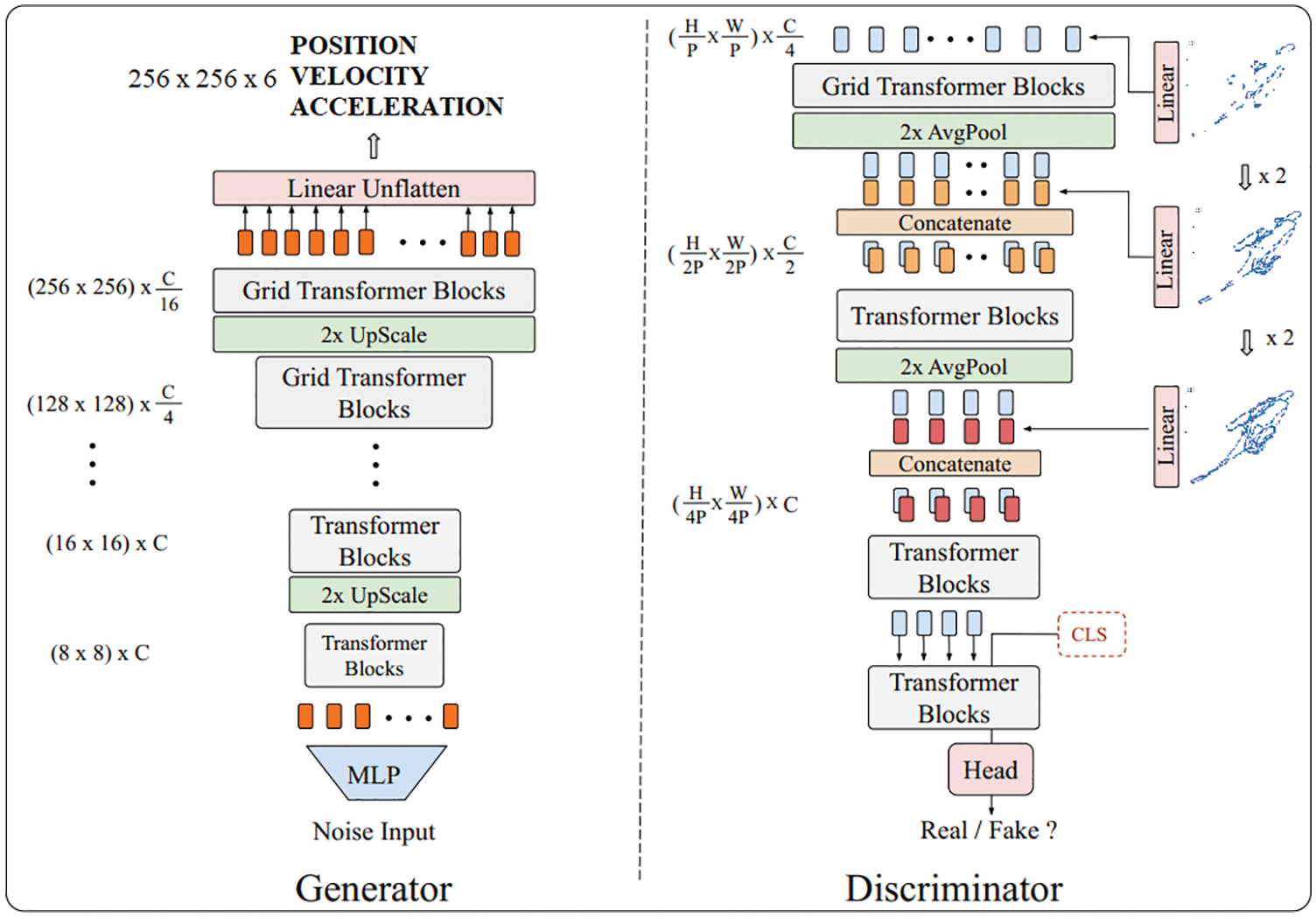
Figure 4: TransGAN model

The basic module of the network generation is transformer encoder, which is improved by replacing the self-coding module with the grid self-coding module. Thus, the memory bottleneck can be further alleviated when TransGAN is extended to high-resolution transforer. For the image task, if the converter is simply used as the generator to generate the image pixel by pixel, its length will also become 1,024 even if the low resolution image (such as 32×32 ) it is extended into a sequence, and the cost of direct self-attention calculation is extremely high. Therefore, TransGAN borrows the idea of CNN and iteratively reduces the embedding dimension to improve the resolution [32]. Specifically, it adopts an up-sampling module composed of a shaping layer and a resolution enhancing layer to improve the resolution. For the low-resolution phase (the resolution lower than 64×64 ), the up-sampling module first shapes the one-dimensional sequence embedded in the token into a two-dimensional feature map (H×W×C) . Then, while keeping the embedding dimension unchanged, the bicubic sampling layer is up-sampled to double the resolution, and the output is 2H×2W×C . Next, the two-dimensional feature mapping is reshaped into a one-dimensional embedded tag sequence again. For the higher resolution stage, the pixel shuffling module is used instead of bicubic layer, which doubles the resolution of feature mapping and reduces the embedded dimension to a quarter of the original one. This step is repeated for several stages until the target resolution is reached.

The discriminator only needs to identify the authenticity of the image, not every pixel. Therefore, the discriminator divides the input two-dimensional image into coarse blocks, and sends them to the converter encoder in combination with the learnable position code. Finally, the true/false classification is output through the fully-connected layer.

3  INS-GNSS Based on TransGAN

3.1 Integrated Navigation Mathematical Model

The inertial state dynamic position error model is as follows [33]:

{ δα˙=δvE(RN+γ)cosβδβ˙=δvNRM+γδγ˙=δvD (13)

The speed error model is as follows [33]:

{δv˙E=(2ϖsin⁡β+vERN+γtan⁡β)vN−(2ϖcos⁡β+vERN+γ)vU+fN+fEδh−fDδl+BNδv˙N=−(2ϖsin⁡β+vERN+γtan⁡β)vE−vNRM+γvU+fE+fNδh−fDδL+BEδv˙D=(2ϖcos⁡β+vERN+γ)vE−vN2RM+γ−g+fD+fEδL−fNδL+BD (14)

In the formula, δvE , δvN , δγ and δβ can be acquired approximately by subtracting the corresponding outputs of INS and GPS. According to the system error equation, the attitude error model can be obtained as follows [33]:

{δL˙=(ϖsin⁡β+vERN+γtan⁡β)l−(ϖcos⁡β+vERN+γ)h+δvNRM+γ−vNδγRM+γ+DNδl˙=−(ϖsin⁡β+vERN+γtan⁡β)L−vNRM+γh−δvERN+γ−vEδγ(RN+γ)2+ϖδβsin⁡β+DEδh˙=(ϖcos⁡β+vERN+γ)L−vNRM+γl−δvERN+γtan⁡β+vEδγtan⁡β(RN+γ)2−(ϖcos⁡β+vEsec2βRN+γ)δβ+DD (15)

where, RM and RN are the radius of curvature in meridional circle and the radius of curvature in unitary circle, respectively; ω denotes the rotational velocity of the earth; g is the acceleration of gravity; vN , vE and vU are the velocities in the north, east and upward directions, respectively; fN , fE and fD are the specific forces of the accelerometer output in the north, east and downward directions, respectively [34]; BN , BE and BD are the deviations of the accelerometer in the north, east and downward directions, respectively; DN , DE and DD are the constant drifts of the gyroscope in the north, east and downward directions, respectively [35].

The first-order Markov models of gyro constant drift and accelerometer deviation are respectively as follows:

{D˙i=−μDi+ρB˙i=0,  i=N,E,D (16)

where μ denotes the correlation coefficient measured by the sensor; ρ denotes zero mean Gaussian white noise [36]. The error model of inertia state dynamics can be expressed in the following state space form:

x˙=f(x,ρ(t),t) (17)

where f(x,ρ(t),t) is a nonlinear continuous function; x is the error state vector of INS, including three position errors, three velocity errors, three attitude errors, three accelerometer errors and three gyro constant drifts; ρ(t) denotes the white noise, including constant drift of accelerometers and gyroscopes. The state vector is defined as Eqs. (18) and (19):

x=(δa,δβ,δγ,δvN,δvE,δvD,δL,δl,δh,BN,BE,BD,DN,DE,DD) (18)

x=(δA,δβ,δγ,δVN,δVe,δVD,δL,δh,BN,be,BD,DN,De,DD) (19)

Eq. (17) is a nonlinear model. In order to apply this model to KF, it needs to be discretized through Eq. (20):

xk+1=J(tk+1−tk)xk+ρk (20)

where J is the state transition matrix; ρk is the Gaussian white noise associated with the inertial sensor. Similarly, the general discrete form of the measurement equation is as follows:

zk=Hkxx+vk (21)

where Hk is the observation matrix; vk is the zero-mean Gaussian measurement noise, and its covariance matrix is R. zk is updated by subtracting the position, speed and heading angle of GNSS from the position, speed and heading angle of INS [37].

Hk=[00000010000000000000001000000000000000100000000010000000000000001000000000000000100000000000−1000000000000] (22)

The nonlinear model Eq. (17) is used as the input of the neural network, which includes PINS , vINS and accelerometer output fNED=((FN,Fe,FD)T) ; The output of linear model Eq. (20) is the input of KF; KF is used to estimate the position error, velocity error, attitude error, accelerometer deviation and gyro constant drift, and subsequently correct the final output of the combined system.

3.2 TransGAN-Assisted INS-GNSS Implementation

There are some defects and limitations in KF algorithm, such as suboptimal or even divergent filter estimation [38]. For low-cost INS-GNSS, the nonlinear error term is ignored in the establishment of KF linear error model, resulting in large positioning error. Therefore, the nonlinear processing of INS-GNSS is realized based on the idea of TransGAN. The most common method is to correlate INS error with output, predict the difference between INS and GNSS output, and then use it as the observation vector of KF. Similarly, the proposed TransGAN is applied to INS-GNSS by using PINS−δPINS and vINS−δvINS . TransGAN-assisted INS-GNSS can continuously provide position and velocity errors during GNSS interruption. The position, velocity and accelerometer outputs of INS are taken as the inputs of the TransGAN generator, and the position error and velocity error corresponding to INS are taken as the outputs of TransGAN generator. In Fig. 5, IMU refers to inertial measurement unit, including gyroscope and accelerometer; AINS=(L,1,h) ; T is the attitude vector. During TransGAN training, the outputs of INS and GNSS are combined by KF when GNSS works normally.

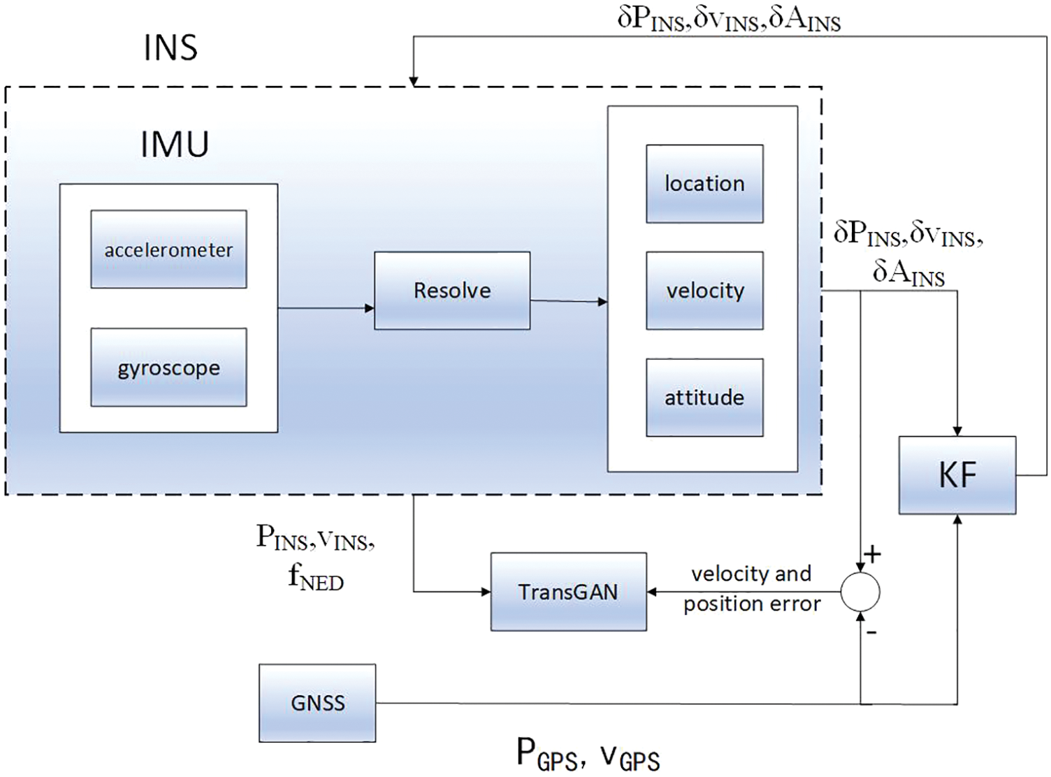
Figure 5: Training process of TransGAN

As shown in Fig. 5, for each INS-GNSS, the output correction is to take the filter estimation as the output of the combined system or as the correction amount of the output of the inertial navigation system to improve the accuracy of the output. Whereas it does not correct the error state inside the inertial navigation system. The error estimation accuracy of the filter determines the accuracy of the correction, whose advantages are that the subsystem and filter work independently, and it is easy to be implemented in engineering. The filter failure will not affect the system work, so the reliability is high. However, the model will change after running for a long time, which will reduce the filtering accuracy. The feedback correction is to feed back the filter estimation to the inertial navigation system and other systems to correct correct the error state, and afterwards the corrected parameters enter the next operation. In the feedback correction mode, the corrected attitude matrix is fed back to the system to participate in the solution, so the system error is always kept small and there will be no model error, so it has higher accuracy. The engineering implementation is complex, and the filter failure will directly affect the system output, thus reducing the reliability.

Using enhanced KF, PINS−δPINS and vINS−δvINS , the structure of INS can be further enhanced, and a robust nonlinear model can be obtained, which provides INS error and accurate positioning information when GNSS is interrupted. When GNSS can receive accurate navigation data, training TransGAN will continuously reduce the estimation error of TransGAN generator to obtain the optimal network factor. The neural network can update the weights of the neural network to recover the acquired navigation knowledge. In the network training mode, the INS position error and velocity error output by the neural network module should be compared with the reference values. The reference velocity error δvINS−GNSS and position error δPINS−GNSS are defined as follows:

{δvINS−GNSS=vINS−vGNSSδPINS−GNSS=PINS−PGNSS (23)

The velocity error and position error of the output of the TransGAN module are the estimation errors of the TransGAN generator module. To reduce this error, TransGAN is trained to correct its factors and update them according to the least square criterion until a certain mean square error is reached. Repeat training for all INS-GNSS information until GNSS interruption is determined. Fig. 6 indicates the TransGAN prediction process during GNSS interruption. When GNSS fails, GNSS cannot provide KF observation vector, so the trained TransGAN generator is used instead of GNSS to predict navigation error. In the prediction mode, the velocity and position information of ins and fNED are the inputs of TransGAN, and the neural network output including the velocity and position error information is fused into KF.

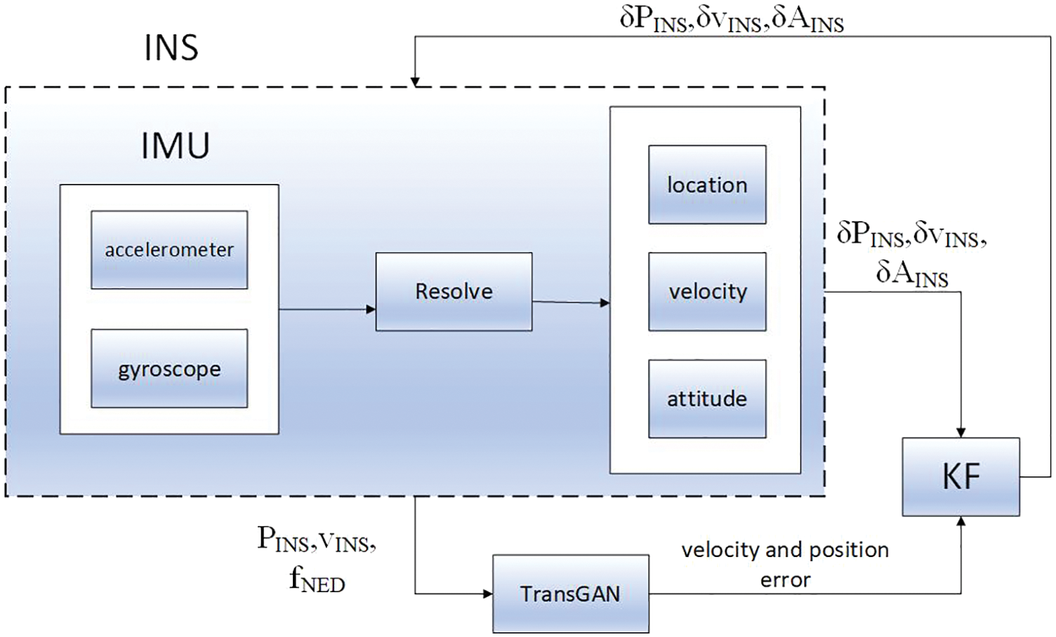
Figure 6: TransGAN prediction process during GNSS interruption

4  Simulation Results and Test Analysis

4.1 Simulation Results

Through the flight test in the waters around Dalian Port, the performance of the integrated navigation system proposed in this paper is evaluated. The trajectory generated by INS-GNSS navigation is shown in Fig. 7. INS generates the original measurement value of IMU, as well as the aircraft position, velocity and attitude data with a sampling frequency of 20 Hz; The GNSS update frequency is 20 Hz. With reference to the baseline GNSS receiver, high-precision data could be obtained through real-time dynamic correction, with the sampling frequency being 100 Hz, and the sampling time being about 1,400 s. In the initial state, INS-GNSS works in the initial alignment mode for 200 s. In order to study the impact of GNSS interruption on system error, and test the navigation error prediction ability of the proposed TransGAN, GNSS is artificially interrupted, as shown in Fig. 8, and two GNSS interruption intervals are generated.

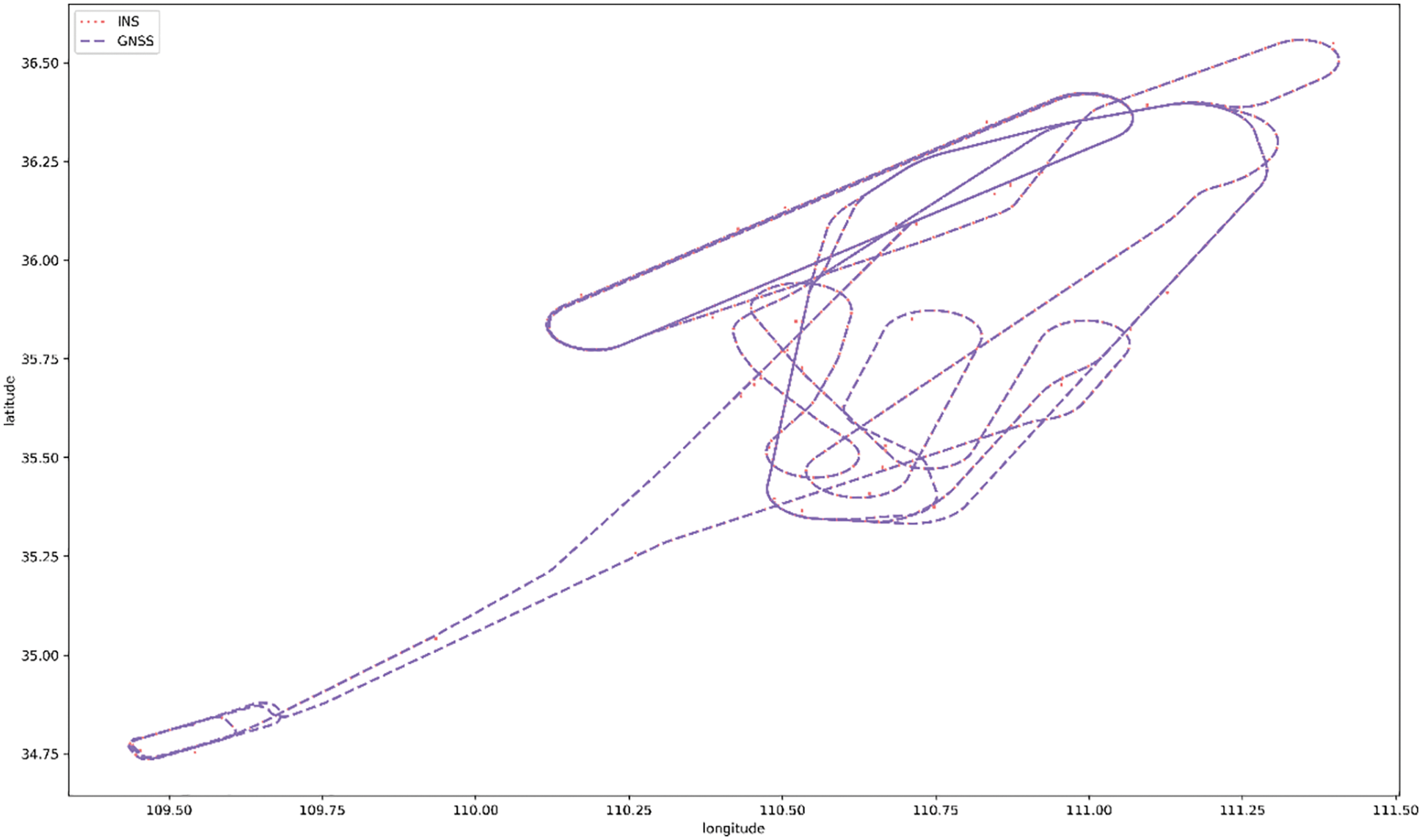
Figure 7: INS/GNSS navigation trajectory

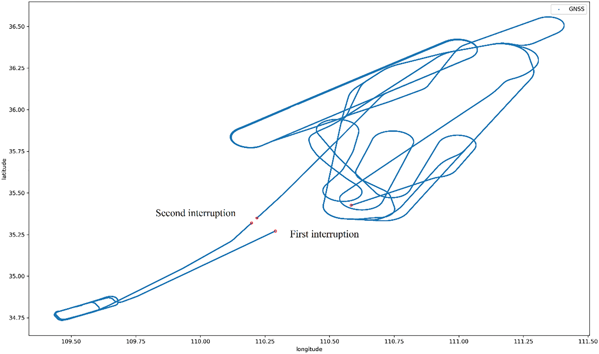
Figure 8: GNSS interrupt trajectory

4.2 Performance Analysis of TransGAN Integrated Navigation Algorithm

As shown in Fig. 9, when the GNSS signal is interrupted, the whole system will switch from the training mode to the prediction mode. The measured values from INS (i.e., specific force, speed, yaw and angular velocity) are sent to the trained TransGAN-based network model as input features, and the predicted value of position increment is obtained through the trained network model. Then, by accumulating these position increments, the pseudo GNSS position observations can be obtained to replace the original real GNSS position observations. After the difference with the position measurement value in INS is continued, the information of Kalman filter can be formed. Later, the error state vector output by the Kalman filter will be used to feedback and correct various errors of INS, so as to obtain the corrected position, velocity and attitude. Six accessible transform neural network modules, including P-δP structure (for estimating position (longitude, latitude and altitude)) and V-δV structure (for estimating the northward velocity component (VN), eastbound velocity component (VE), and the upward velocity component (VU)). Each neural network module has four input layer neurons (including one velocity or position component and three accelerations) and one output layer neuron (for providing velocity error and position error).

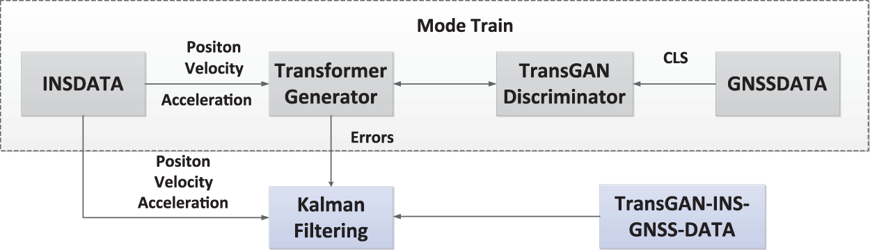
Figure 9: Flow chart of INS-GNSS integrated navigation algorithm based on TransGAN

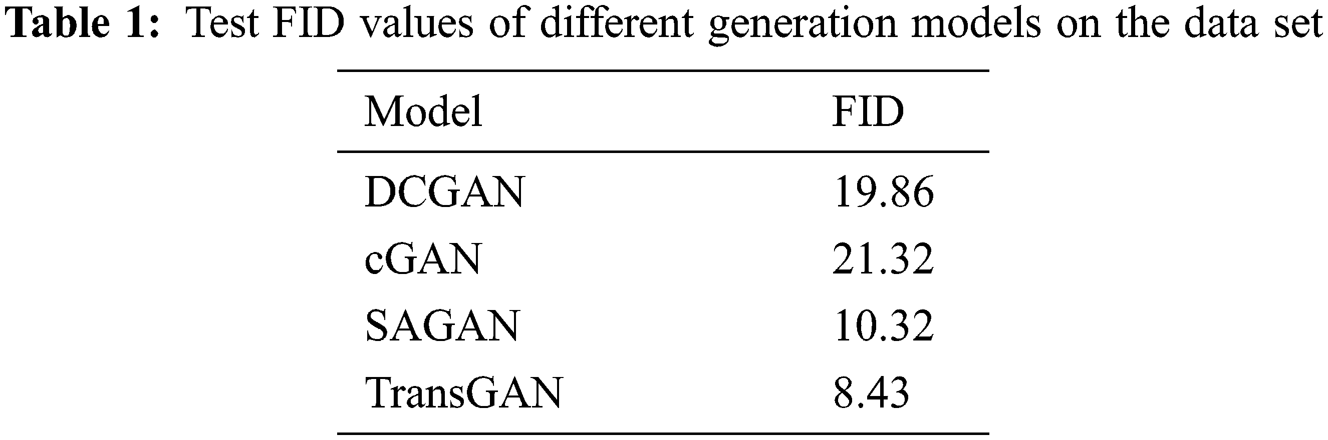
In order to evaluate the quality of the generated image, the Frechette Start Distance (FID) is used as the evaluation index. FID is a principled comprehensive index. The lower the value, the closer the data distribution will be to the real data distribution, that is, the more realistic the image will be.

Training and testing were performed on the dataset and the ability of these depth models to generate tagged data was evaluated by calculating FID values for Deep Convolutional Generative Adversarial Network (DCGAN), Conditional Generative Adversarial Networks (cGAN), Self-Attention GAN (SAGAN), and TransGAN. Table 1 lists the results of training and testing on datasets by TransGAN compared with several other commonly used generation models. The results show that TransGAN can improve the quality of generated data and lay a foundation for improving the combined positioning accuracy.

The GNSS interrupts for the first time at 2,568~753 s, when the plane flies at a speed of 591 km/h, and is in a acceleration state; The GNSS interrupts for the second time at 17,217~17,252 s, when it flies at a speed of 459 km/h, and the ship is in a deceleration state. During the uninterrupted process of GNSS, the test information collected from INS and GNSS is used to train TransGAN, and then the trained genetic neural network is used to estimate the position error and velocity error from 2,568 to 2,753 s. Fig. 10 shows the training curve of the P-δP module of the ship position (longitude, latitude and altitude) before the first GNSS interruption, with the target mean square error of 000001. The training process of V-δV module is similar to that of P-δP module, so only the training curve of P-δP module is given here.

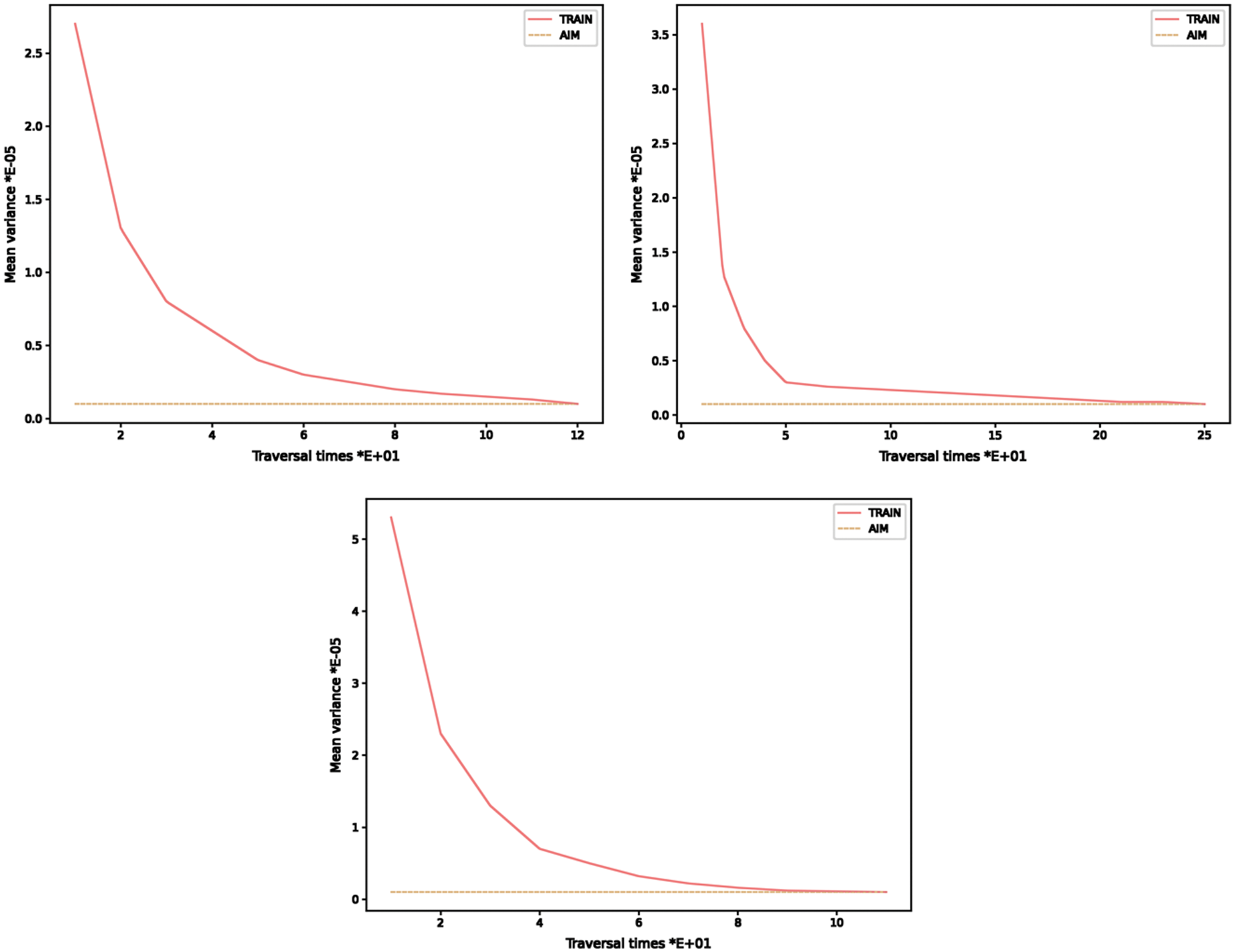
Figure 10: Training curve of aircraft position data under normal GNSS

To verify the applicability of the algorithm, the estimation results of position and velocity components of TransGAN-assisted INS-GNSS, GNSS and traditional KF during GNSS interruption are compared. It should be noted that the position, velocity and heading angle data from GNSS are unreliable during GNSS interruption, so there is no observation vector of KF [39]. Fig. 11 shows the position and velocity estimation curves during GNSS interruption. As can be seen from it, the proposed TransGAN-assisted KF algorithm has favorable performance in position and velocity estimation. The results show that the INS error could be effectively compensated when the GNSS signal is interrupted, mainly because the navigation system based on TransGAN network can capture intelligent information according to the training period of the test path, thus reducing the positioning error.

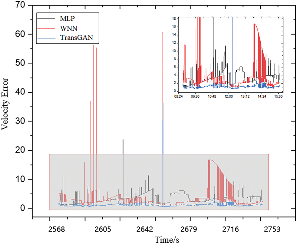
Figure 11: Aircraft position data quality curve during the first GNSS interruption

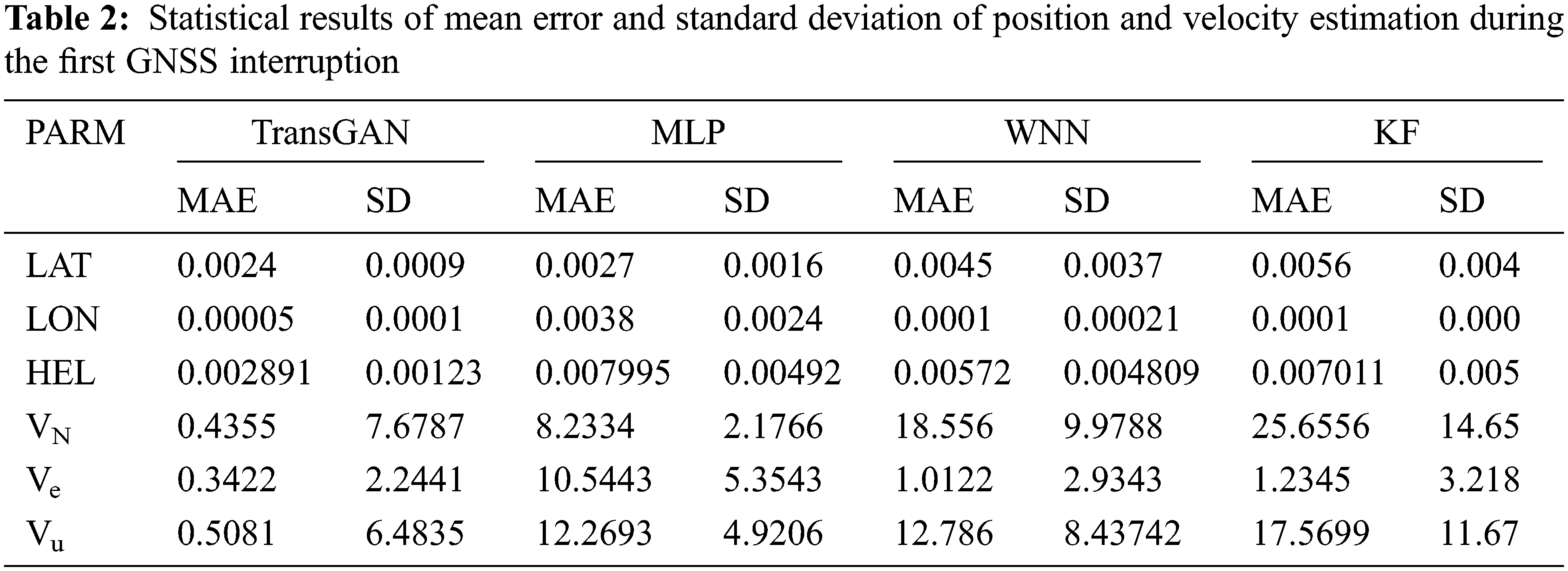
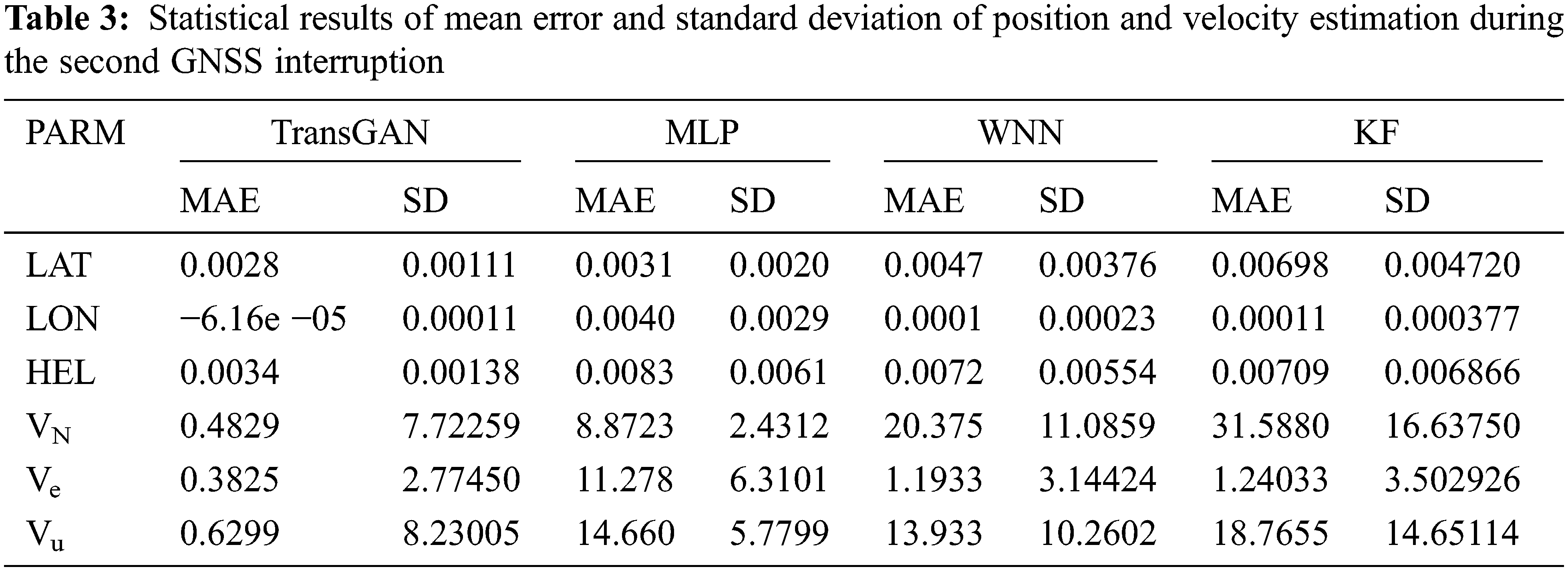
In order to verify the effectiveness of the proposed TransGAN, its performance is compared with that of the traditional MLP and WNN. The MLP consists of two hidden layers and a four-layer WNN. The input and output of MLP and WNN are the same as those of TransGAN, taking a four-dimensional vector as the input, mapping it to the hidden layer, and finally outputting a one-dimensional vector [40]. For better estimation, Tables 2 and 3 present the statistical results of mean error and standard deviation of position and velocity estimation based on the same set of test data during two GNSS interruptions. It can be seen from Tables 2 and 3 that compared with MLP, WNN and KF, TransGAN has significantly lower mean error and standard deviation of position and velocity estimation.

As shown in Fig. 11, the test results display that since MLP and WNN models do not have a parameter updating process in time latitude, they cannot handle the time correlation between current and past vehicle dynamics, so they cannot be used as suitable models to assist INS during GNSS signal interruption. When the GNSS signal is lost, the transformer-based generation algorithm is capable of building the relationship between future and past information, so more accurate navigation results can be obtained. The performance of INS/GNSS integrated navigation based on TransGAN is greatly improved on the basis of GNSS direction finding, which can meet the requirements of high accuracy and high performance when GNSS is interrupted. In addition to the advantages of conventional integrated navigation, the TransGAN model not only accelerates the convergence speed and reduces the iteration times, but also effectively improves the accuracy of GNSS data reconstruction, improves the dimension of KF input data, solves the shortcomings of inaccurate INS data, and improves the accuracy of initial motion alignment of the carrier. On the other hand, from the error results of several combination methods, it can be seen that the TransGAN-assisted Kalman filter can effectively restrain error divergence and provide more accurate navigation results. Moreover, compared with the standard Kalman filter, the error fluctuation range of the integrated navigation algorithm based on TransGAN is greatly reduced, and the influence of observation information errors and dynamic model anomalies can be better controlled.

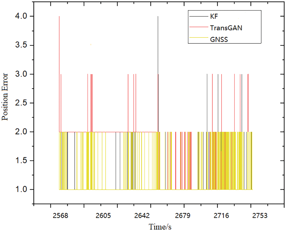
Figure 12: Error comparison of several integrated navigation methods

5  Conclusion

With the advancement of artificial neural network, the optimizing algorithm of integrated navigation system have achieved remarkable results [41]. Based on artificial neural network technology, an integrated navigation system INS-GNSS is proposed. The performance of the navigation system is evaluated through flight tests. The navigation system uses the position and speed of GNSS to assist INS. When GNSS is working normally, position, speed and error results are used to assist INS; When GNSS is interrupted, TransGAN is applied to reduce the accumulation of velocity and position errors of INS-GNSS. When GNSS works normally, the velocity, position, specific force and GNSS data of INS are employed to train TransGAN; During the interruption of GNSS, the trained TransGAN provides accurate position and velocity error values as KF observations to reduce the estimation errors of INS. Experiments show that TransGAN-assisted INS-GNSS has significantly lower speed and position prediction errors during GNSS interruption than that in MLP, WNN and KF.

In recent years, the research of multi-source integrated navigation systems has developed rapidly, but now most navigation systems rely on the combination of GNSS and INS, generally one or more additional special auxiliary sensors to provide accurate positioning and navigation information. These systems obtain “point solutions” by optimizing specific sensors and measurement sources. The problem with this processing method is that it is not flexible enough to adapt to new threats or task challenges. By using information extracted from different combinations of auxiliary sensors, such as LIDARS, laser rangefinders, cameras and magnetometers, the quality and robustness of navigation solutions can be enhanced. The opportunity signals (SoOPs) and natural phenomena from the existing RF background infrastructure are also useful, and new measurement sources are constantly being explored.

Funding Statement: The authors received no specific funding for this study.

Conflicts of Interest: The authors declare that they have no conflicts of interest to report regarding the present study.

References

1. C. Zhang, C. Q. Xiong and L. Y. Wang, “A research on generative adversarial networks applied to text generation,” in Proc. 14th Int. Conf. on Computer Science and Education (ICCSE), Toronto, TO, Canada, pp. 913–917, 2020. [Google Scholar]

2. G. Guarino, A. Samet and A. Nafi, “PaGAN: Generative adversarial network for patent understanding,” in Proc. 21st IEEE Int. Conf. on Data Mining (ICDMBarcelona, Barca, Spain, pp. 1084–1089, 2022. [Google Scholar]

3. S. F. Wu, X. Xiao and Q. G. Ding, “Adversarial sparse transformer for time series forecasting,” in Proc. 34th Conf. on Neural Information Processing Systems (NeurIPSVancouver, Van, Canada, pp. 43–47, 2020. [Google Scholar]

4. C. Y. Wang, C. Xu and X. Yao, “Evolutionary generative adversarial networks,” IEEE Transactions on Evolutionary Computation, vol. 33, no. 6, pp. 921–934, 2020. [Google Scholar]

5. M. Azzam, W. Wu, W. Cao and S. Wu, “KTransGAN: Variational inference-based knowledge transfer for unsupervised conditional generative learning,” IEEE Transactions on Multimedia, vol. 23, no. 5, pp. 3318–3331, 2020. [Google Scholar]

6. Y. Jiang, S. Chang and Z. Wang, “TransGAN: Two pure transformers can make one strong GAN, and that can scale up,” in Proc. 35th Conf. on Neural Information Processing Systems (NeurIPS), Montreal, MTL, Canada, 2021. [Google Scholar]

7. C. Zhang, C. Guo and G. D. Zhan, “Ship navigation via GPS/IMU/LOG integration using adaptive fission particle filter,” Ocean Engineering, vol. 156, no. 7, pp. 435–445, 2018. [Google Scholar]

8. M. Ismail and Y. E. Abdelkaw, “Hybrid error modeling for MEMS IMU in integrated GPS/INS navigation system,” The Journal of Global Positioning Systems, vol. 16, no. 1, pp. 1–12, 2018. [Google Scholar]

9. K. W. Chiang, A. Noureldin and N. Eisheimy, “Multisensor integration using neuron computing for land-vehicle navigation,” GPS Solutions, vol. 6, no. 4, pp. 209–218, 2003. [Google Scholar]

10. A. Noureldin, A. Osman and N. Elsheimy, “A neuro-wavelet method for multi-sensor system integration for vehicular navigation,” Measurement Science and Technology, vol. 51, no. 4, pp. 259–268, 2004. [Google Scholar]

11. S. Chen, Y. Hung and C. Wu, “Application of a recurrent wavelet fuzzy-neural network in the positioning control of a magnetic-bearing mechanism,” Computer Electrical Engineering, vol. 54, no. 5, pp. 147–158, 2016. [Google Scholar]

12. S. Cheng, L. Li and J. Chen, “Fusion algorithm design based on adaptive SCKF and integral correction for side-slip angle observation,” IEEE Transactions on Industrial Electronics, vol. 65, no. 1, pp. 5754–5763, 2018. [Google Scholar]

13. J. Li, N. F. Song, G. L. Yang and M. Li, “Improving positioning accuracy of vehicular navigation system during GPS outages utilizing ensemble learning algorithm,” Information Fusion, vol. 35, no. 3, pp. 1–10, 2017. [Google Scholar]

14. M. Majid, K. Mojtaba, C. Rupp and D. Ting, “Power production prediction of wind turbines using fusion of MLP and ANFIS networks,” IET Renewable Power Generation, vol. 12, no. 9, pp. 1025–1033, 2018. [Google Scholar]

15. B. Huang, W. Chen, X. Wu, C. Lin and P. N. Suganthan, “High-quality face image generated with conditional boundary equilibrium generative adversarial networks,” Pattern Recognition Letters, vol. 111, no. 8, pp. 72–79, 2018. [Google Scholar]

16. C. Xiao, B. Li, J. Y. Zhu, W. He, M. Liu et al., “Generating adversarial examples with adversarial networks,” in Proc. Generating Adversarial Examples with Adversarial Networks (IJCAI), Stockholm, STO, Sweden, pp. 3905–3911, 2018. [Google Scholar]

17. J. Liu, C. K. Gu, J. Wang, G. Youn and J. U. Kim, “Multi-scale multi-class conditional generative adversarial network for handwritten character generation,” Journal of Supercomputing, vol. 75, no. 4, pp. 1922–1940, 2019. [Google Scholar]

18. L. F. Zhang, S. P. Wang, M. S. Selezneva and K. A. Neusypin, “A new adaptive Kalman filter for navigation systems of carrier-based aircraft,” Chinese Journal of Aeronautics, vol. 35, no. 1, pp. 416–425, 2022. [Google Scholar]

19. L. Yann, B. Yoshua and H. Geoffrey, “Deep learning,” Nature, vol. 521, no. 7553, pp. 436–444, 2015. [Google Scholar]

20. M. Roopaei, P. Rad and M. Jamshidi, “Deep learning control for complex and large scale cloud systems,” Intelligent Automation and Soft Computing, vol. 23, no. 3, pp. 389–391, 2018. [Google Scholar]

21. L. A. Gatys, A. S. Ecker, M. Bethge, A. Hertzmann and E. Shechtman, “Controlling perceptual factors in neural style transfer,” in Proc. IEEE Int. Conf. on Computer Vision (CVPR), Hawaii, HI, USA, pp. 3730–3738, 2017. [Google Scholar]

22. S. R. Zhou, M. L. Ke and P. Luo, “Multi-camera transfer GAN for person re-identification,” Journal of Visual Communication and Image Representation, vol. 59, no. 1, pp. 393–400, 2019. [Google Scholar]

23. X. Chen, Y. Duan, R. J. Houthooft, I. Schulman and P. Sutskever, “Interpretable representation learning by information maximizing generative adversarial nets,” in Proc. of the Advances in Neural Information Processing Systems, Barcelona, BCN, Spain, pp. 2172–2180, 2016. [Google Scholar]

24. M. Mehraliamamd and K. Karas, “B.RDCGAN: Unsupervised representation learning with regularized deep convolutional generative adversarial networks,” in Proc. 2018 9th. Conf. on Artificial Intelligence and Robotics and 2nd Asia-Pacific Int. Symp. (AAAI), Kish, KIH, Iran, pp. 88–95, 2018. [Google Scholar]

25. A. Madry, A. Makelov, L. Schmidt, D. Tsipras and A. Vladu, “Towards deep learning models resistant to adversarial attacks,” in Proc. 2018 Int. Conf. on Learning Representations (ICLR), Vancouver, Van, Canada, pp. 542–554, 2018. [Google Scholar]

26. X. Mao, S. Wang, L. Zheng and Q. Huang, “Semantic invariant cross-domain image generation with generative adversarial networks,” Neurocomputing, vol. 293, no. 7, pp. 55–63, 2018. [Google Scholar]

27. X. Chen, Y. Duan, R. Houthooft, J. Schulman, I. Sutskever et al., “Infogan: Interpretable representation learning by information maximizing generative adversarial nets,” in Proc. Advances in Neural Information Processing Systems, Barcelona, BCN, Spain, pp. 2172–2180, 2021. [Google Scholar]

28. Z. Zhang, Q. Liu and Y. Wang, “Road extraction by deep residual U-Net,” IEEE Geoscience and Remote Sensing Letters, vol. 15, no. 5, pp. 1749–1753, 2018. [Google Scholar]

29. M. M. Li, Y. F and X. X. Y, “Adaptive relative navigation based on cubature Kalman filter,” Aero-Space Control, vol. 33, no. 1, pp. 43–47, 2015. [Google Scholar]

30. I. J. Goodfellow, J. Pouget-Abadie, M. Mirza, B. Xu and F. David, “Generative adversarial networks,” Advances in Neural Information Processing Systems, vol. 3, no. 2, pp. 2672–2680, 2014. [Google Scholar]

31. D. Holden, I. Habibie and I. Kusajima, “Fast neural style transfer for motion data,” IEEE Computer Graphics & Applications, vol. 37, no. 4, pp. 42–49, 2017. [Google Scholar]

32. C. Q. Wang, A. G. Xu, X. Sui, Y. S. Hao and Z. X. Shi, “A seamless navigation system and applications for autonomous vehicles using a tightly coupled GNSS/UWB/INS/Map integration scheme,” Remote Sensing, vol. 14, no. 1, pp. 1–25, 2022. [Google Scholar]

33. K. W. Chiang, G. J. Tsai and H. J. Chu, “Performance enhancement of INS/GNSS/Refreshed-SLAM integration for acceptable lane-level navigation accuracy,” IEEE Transactions on Vehicular Technology, vol. 69, no. 3, pp. 2463–2476, 2020. [Google Scholar]

34. C. Jiang, S. Chen, Y. Chen and Y. Bo, “Research on a chip scale atomic clock driven GNSS/SINS deeply coupled navigation system for augmented performance,” IET Radar Sonar & Navigation, vol. 13, no. 2, pp. 326–331, 2018. [Google Scholar]

35. D. Narjes and G. Asghar, “An asynchronous adaptive direct Kalman filter algorithm to improve underwater navigation system performance,” IEEE Sensors Journal, vol. 17, no. 4, pp. 1061–1068, 2017. [Google Scholar]

36. H. Zhao, J. Xing and M. Qiu, “Estimate of initial installation angle of INS in vehicle MEMS-INS/GNSS integrated navigation system,” in China Satellite Navigation Conf., Nanchang, NC, China, pp. 606–621, 2021. [Google Scholar]

37. R. Sharaf, A. Nourledin and A. Osman, “Online INS/GNSS integration with a radial basis function neural network,” IEEE Aerospace & Electronic Systems Magazine, vol. 20, no. 3, pp. 8–14, 2005. [Google Scholar]

38. X. Cai, H. Hsu and H. Chai, “Multi-antenna GNSS and INS integrated position and attitude determination without base station for land vehicles,” The Journal of Navigation, vol. 72, no. 2, pp. 342–358, 2019. [Google Scholar]

39. H. Nourmohammadi and J. Keighobadi, “Fuzzy adaptive integration scheme for low-cost SINS/GPS navigation system,” Mechanical Systems and Signal Processing, vol. 99, no. 15, pp. 434–449, 2018. [Google Scholar]

40. F. Zhou, L. Y. Liang and P. Lin, “Research on INS/GNSS/RADAR integrated navigation with covariance intersection fusion,” Aerospace Control, vol. 39, no. 4, pp. 22–27, 2021. [Google Scholar]

41. W. Sun, G. Z. Dai, X. R. Zhang, X. Z. He and X. Chen, “TBE-Net: A three-branch embedding network with part-aware ability and feature complementary learning for vehicle re-identification,” IEEE Transactions on Intelligent Transportation Systems, vol. 23, no. 9, pp. 14557–14569, 2022. [Google Scholar]