Detection Algorithm of Knee Osteoarthritis Based on Magnetic Resonance Images

1  Introduction

Knee osteoarthritis (OA) is the degeneration of articular cartilage caused by chronic strain. Knee OA is highly prevalent in the elderly, obese, and sedentary people, and can lead to joint pain, limited mobility, and even disability. At present, hip OA and knee OA are ranked eleventh in the global ranking of disabilities. World Health Organization statistics show that the prevalence of knee OA can be as high as 50% in the people over the age of 50 and as high as 80% in the people over the period of 75 [1]. Generally, advanced knee OA can only be treated with total knee arthroplasty. Therefore, early detection and intervention can help slow down OA degeneration [2]. Although X-ray has been widely used in the computer-aided diagnosis of knee OA, X-ray images are insensitive when diagnosing and detecting early changes in knee OA [3]. Magnetic resonance (MR) imaging can better present soft tissues such as cartilage, myelopathy, and effusion. It can provide significant greatly help for the early diagnosis of knee OA [4]. Therefore, in our study, the detection method based on MR images of knee joints was proposed to identify whether there is knee OA or not.

The primary contributions of this paper are the use of knee MR images to perform knee OA detection. Compared to the previous study, for the first time, we introduce a deep transfer learning method to classify knee OA and design a block-by-block fine-tuning strategy for training. We show that adding more dense blocks in fine-tuning can make the model obtain better detection performance. We perform an extensive experimental validation of the proposed method using various metrics and explore the influence of the network’s depth on the performance. Our approach performs well, which shows that MR images have more tremendous potential to improve diagnostic accuracy for knee OA.

The structure of this paper is as follows: Section two elaborates on the principle and implementation process of the algorithm. In section three, the comparative experiment was carried out, and the results are presented on the OAI-ZIB dataset. Section four summarizes the work.

2  Related Works

At present, the detection of knee OA mainly focuses on X-ray images. Woloszynski et al. [5] used the Signature Dissimilarity Measure (SDM) to classify the texture of nodules in knee radiographs. With the rapid development of deep learning applications in computer vision and other research fields, satisfactory results of knee OA detection based on x-ray images have been obtained by Convolutional Neural Networks (CNN). Antony et al. [6] used a VGG16 network model pre-trained on ImageNet to grade knee OA. Later, Antony et al. [7] combined fully convolutional neural networks (FCNs) with lightweight network models to localize knee joints and classify knee joint OA. Tiulpin et al. [8] exploited the symmetry of the images and adopted a deep Siamese network model to classify knee OA. Chen et al. [9] adopted the YOLOv2 network to detect knee joints. They fine-tuned popular CNN models such as VGG, Inception v3, etc. A novel adjustable ordinal loss is applied to knee OA classification. Currently, in clinical practice, doctors usually use x-rays to check the graded diagnosis of knee OA. While, the structural changes visible on X-rays, such as skeletal abnormalities and Narrowing of Joint Space (JSN), a pathological form of cartilage thinning and meniscal herniation, appear only in relatively advanced stages of the disease. So the accuracy of knee OA detection based on X-ray needs to be improved.

MR images can better present soft tissues such as cartilage, bone marrow lesions, and effusion, which can help the early diagnosis of knee OA. However, the current research on knee OA based on MR images is still focused on prediction and segmentation. Wang et al. [10] applied a 3D CNN model to calculate the probability of requiring total knee replacement (TKR) in the next nine years based on the severity of OA; Panfilov et al. [11] used 2D CNN and a Transformer network model to predict whether knee OA will occur in the next eight years (96 months); Pedoia et al. [12] segmented knee cartilage and meniscus using the popular 2D U-Net network architecture. Wilson et al. [13] quantify spatial gradients and patterns in MR image data, and probe new candidate biomarkers for early severity of OA. Xue et al. [14] developed an MR imaging-based radiomics predictive model for identifying knee OA based on the tibial and femoral subchondral bone. They scanned 88 knees with 3T MR images and manually extracted four trabecular structural parameters and 93 radionics features to identify knee OA with a support vector machine model. Guida et al. [15] utilize a 3D CNN model to analyze sequences of knee MR images to perform knee OA classification according to Kellgren and Lawrence (KL) grade of severity. Compared with a CNN model using X-ray images trained from the same group of patients, the proposed 3D model with MR images achieved higher accuracy in the 5-category classification (54.0% vs. 50.0%) on the testing set. Karim et al. [16] proposed DeepKneeExplainer to leverage explainable knee OA diagnosis based on radiographs and MR images. Experiments were performed on the multicenter osteoarthritis study (MOST) cohorts to predict OA severity level with an accuracy of 91%. Peuna et al. [17] introduced the Grey-Level Co-occurrence Matrix (GLCM) and local binary pattern (LBP) texture analysis to discriminate OA subjects. T2 relaxation time mapping with multi-slice multi-echo spin echo sequence was performed for 80 symptomatic OA patients and 63 asymptomatic controls on a 3T clinical MR images scanner. Relaxation time maps were subjected to GLCM and LBP texture analysis. The best performance was obtained with a multilayer perceptron-type classifier with an overall accuracy of 90.2%.

Roemer et al. [18] believe that knee MR images are more beneficial than X-rays for early diagnosis of knee OA. MR scanning is the most accurate way to assess knee OA. It isn't easy to directly use deep CNN trained from scratch to classify the knee OA, because a large amount of labeled training data are required to ensure that the model can achieve convergence. However, in the medical imaging problem, commonly, there are no large-scale labeled datasets available. The lack of data is one of the restricting factors to improving detection accuracy. To solve this problem, the knee OA detection of MR images based on the transfer learning method is proposed for the first time in this paper. This method can well solve the problem of an insufficient MR images. Therefore, the two-stage training method of the transfer learning model based on DenseNet201 is presented in this paper based on MR images to classify the presence or absence of knee OA.

3  Materials and Methods

3.1 Dataset

This study used the OAI-ZIB dataset (doi.org/10.12752/4.ATEZ.1.0) to classify and diagnose knee MR images. The 3D double-echo steady-state (DESS) MR images data for each knee contains 160 2D image sequences. The example diagrams of healthy knee OA (Non-OA) and diseased knee OA (OA) are shown in Fig. 1. Two groups of subjects with the same number of knee MR images were selected by us. That is, 60 healthy and 60 diseased knee OA subjects were selected.

Figure 1: The example diagrams of knee osteoarthritis and none knee osteoarthritis

3.2 Data Preprocessing

3.2.1 Localization of Cartilage Regions

MR images of the knee joint contain large bony regions and many other tissues, as shown in Fig. 2. An important indicator for the detection and diagnosis of knee OA is usually the cartilaginous area between the femur and tibia (circled position in Fig. 2). Therefore, we use the method of U-Net architecture with ResNet backbone in the literature [16] to automatically extract the cartilage region of the knee joint, that is, the region of interest (ROI) to reduce the input dimension of the image. Finally, the size of our extracted ROI area is 224 × 224, as shown in Fig. 3.

Figure 2: The 2D slices examples of a 3D knee MR image sequence

Figure 3: Example of clipping slice for ROI area of size 224 × 224

3.2.2 Slice Selection

Each sample in the database contains a sequence of 160 MR images. The input dimension of the cropped 224 × 224 × 160 is still high. To further reduce the dimension of the input data, we removed some outer and center slices and some start and end slices in which the bone or cartilage information are missing. The reason for removing the central slices is that they show the transition of the medial and lateral bones, which have indistinct cartilage areas and blurred bony borders. Examples of slices are provided in Fig. 4. The total bone area exists from slice #31. The slice #40 and slice #60 have a larger bone with clear bone boundaries and cartilage. Slice #80 is in the transition range, and the bounder between cartilage and bone is less clear [19]. Therefore, for each sequence, we excluded the first 30 slices (1–30), the middle 20 slices (71–90), and the last 50 slices (111–160). The remaining 60 slices (31–70, 91–110) were input into a convolutional neural network model for detection.

Figure 4: The sample of the selected MR images slices

3.3 Data Normalization and Augmentation

A common dataset partitioning method in machine learning is to divide the available dataset into three subsets, namely training set, validation set, and test set [20]. The machine learning model is learned from the training set. The parameters are adjusted by the validation set during the training process. To get the final model, multiple iterations are performed. Finally, a test set is adopted to measure the model performance after training.

In this study, the data set is divided based on the ratio of training set: validation set: test set = 6:2:2 to guarantee that the slices of the patients in the training set and the test set do not overlap. That is, all the slices of the same patient are either in the training set or in the test set. The data set distribution is shown in Table 1. During the training, to avoid the problem of overfitting, data augmentation operations, such as horizontal flipping, image rotation, and offset, are performed. The parameter values of the augmentation are listed in Table 2.

3.4 Deep Transfer Learning Model Based on DenseNet201

The DenseNet201 [21] network utilizes a dense network to obtain an easy-to-train and highly parameterized, high-efficiency model. Compared with traditional CNNs, DenseNet does not have redundant learned feature maps and requires fewer parameters. The performance of the entire model is significantly increased by feature reuse belonging to different layers [22]. In addition, the dense connections have a regularizing effect, which reduces overfitting tasks with the smaller training sets by applying regularization. Therefore, this paper performs transfer learning based on the DenseNet201 network model.

Transfer learning is a popular method in the field of machine learning. In the process of transfer learning, the pre-trained weights of the model are used to accelerate the training process. By taking the place of the fully connected layer, better detection performance can be obtained. The transfer learning method based on the DenseNet201 model is designed. The DenseNet201 network is pre-trained on the ImageNet public dataset. After pre-training, the initial network weights on the ImageNet and the corresponding model structure are obtained, and applied to the knee MR image by transfer learning. The schematic diagram of transfer learning is shown in Fig. 5.

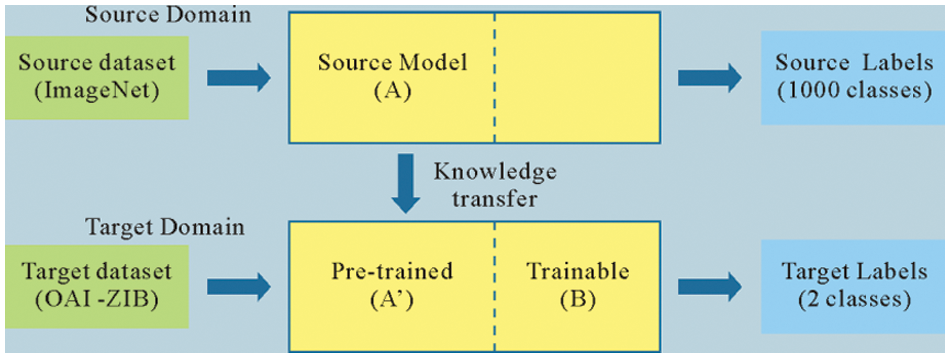
Figure 5: The schematic diagram of transfer learning

The DenseNet201 network model contains four dense blocks, named B1, B2, B3, and B4. Each dense block contains a different number of convolutional blocks. The numbers of convolutional blocks are 6, 12, 48, and 32, respectively. After feature extraction, a three-layer fully connected neural network (B5) is added to replace the original detection layer. Among them, 1024 neurons are used on the first and second fully-connected layers. Since the third fully-connected layer is used aiming at to detect, the number of neurons is 2. After the third fully-connected layer is the Softmax activation function, which produces a probability value between 0 and 1 to determine the class to that the network's output belongs. The Dropout (0.1) layer is inserted between the second fully connected layer and the third fully connected layer to prevent the model from overfitting. The structural parameters of the transfer learning model are shown in Table 3, and the corresponding network architecture diagram is shown in Fig. 6.

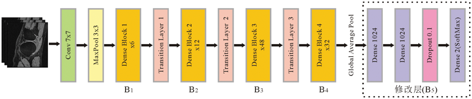
Figure 6: The network architecture of the DenseNet201 based on transfer learning

To extract more features of the knee MR images, the two-stage training process is designed, namely “frozen base layers training” and “block-wise fine-tuning training.” In the first stage, three fully connected layers and one Dropout layer (named B5) are embedded into the DenseNet201 network. All the base layers are frozen, and the weights of B5 are optimized. In the second stage, to further improve the detection accuracy, part of the base layers are unfrozen and trained, together with the weights of B5. During the training of the second stage, if fine-tuning is performed layer-by-layer, the number of times required for fine-tuning will be significantly increased. To improve the training speed, we design a block-by-block fine-tuning method, starting from the last block (B5) for fine-tuning model training. Ten epochs of training are all required in the first and second stages.

4  Experimental Results and Discussion

4.1 Experimental Parameter Settings

In this paper, the optimal detection model for knee OA is designed for MR images. We determine the learning rate (1e-5), batch size (4), and dropout (0.1). In the proposed MR image-based knee OA detection method, the training is accomplished by designing a two-stage training method using the RMSprop optimizer.

The Keras library is used with the framework Tensorflow2.0. The Python programming language is applied to realize the detection of knee OA based on MR images. The training was implemented on a computer equipped with NVIDIA RTX 3090 GPU and Linux operating system.

4.2 Model Evaluation Metrics

The metrics are described below to measure the detection performance. In this study, The metrics including Accuracy (ACC), Precision (PRE), Sensitivity (SEN), Specificity (SPE), F1-Score, and Matthews Correlation Coefficient (MCC) [23,24] are adopted to assess the model performance. The above indicators are defined as follows:

ACC=TP+TNTP+TN+FP+FN(1)

SEN=TPTP+FN(2)

PRE=TPTP+FP(3)

SPE=TNTN+FP(4)

F1−Score=2×(PRE×SEN)(PRE+SEN)(5)

MCC=((TP×TN)−(FP×FN))((TP+FP)(TP+FN)(TN+FP)(TN+FN)(6)

Among them, TP is true positive, FN is false negative, FP is false positive, and TN is true negative.

4.3 Experimental Results and Discussion

Fig. 7 shows the training process of different depth modules. In each subplot of Fig. 7, the abscissa is an epoch, and the ordinate is accuracy and loss, respectively. The black curves (with circle markers) represent the accuracy and loss respectively on the training set only through the first stage training (freezing all base layers, Frozen), while the black curves (with triangle markers) represent the accuracy and loss on the validation set. The green curves (with circle markers) show the accuracy and loss on the training set after the second stage training (fine-tuning, Tuned), while the green curves (with triangle markers) show the accuracy and loss on the validation set.

Figure 7: The accuracy and loss curves corresponding to different depth modules

The performance gap between the shallow and the deep fine-tuning can be seen in Fig. 7. The shallow fine-tuning only tunes the embedding neural network (corresponding to B5 in this paper). The early layers of the CNN involved in deep fine-tuning can determine the low-level features, such as edges, contours, etc, and the later layers determine the high-level features, which can bring more information related to specific detection tasks [25]. Different from the ImageNet dataset, our database corresponds to medical images. It is difficult to learn the complete features of knee MR images with only shallow fine-tuning. The same conclusion is also drawn from the experimental results. The results of the shallow fine-tuning are shown in Fig. 7e. The accuracy after 20 epochs is lower than the other subgraphs, while the loss is higher than the other subgraphs. Therefore, to obtain better model detection performance, it is essential to perform deep fine-tuning of the model and gradually add more dense blocks. After the fine-tuning (seen in Figs. 7a–7d), both the convergence speed and the detection accuracy are significantly improved.

The evaluation indicators on the test set corresponding to the modules with different tuning depths are listed in Table 4. The corresponding histogram is given in Fig. 8.

Figure 8: Evaluation index map corresponding to different depth modules

It can be seen from Fig. 8 that the evaluation index values obtained by the deep fine-tuning B1→B5 module are the highest. When the shallow fine-tuning of module B5 is performed, the obtained evaluation index value is the lowest. As seen from Table 4, the values of all the evaluation indicators are the highest (bold) when unfreezing all the dense blocks and training them together with the weights of the embedding neural network (i.e., the model is deeply fine-tuned for B1→B5). The obtained accuracy, sensitivity, precision, specificity, F1-Score, and MCC were 0.921, 0.960, 0.885, 0.891, 0.912, 0.836, respectively. While freezing all the dense blocks layers and only training the weights of the embedding neural networks B5, the value of each evaluation indicator is the lowest. The corresponding evaluation indicators drop to 0.880, 0.910, 0.842, 0.859, 0.874, and 0.758, respectively.

4.4 Comparison Experiments

To demonstrate the superiority of our algorithm in the knee OA of MR images, on the same dataset OAI-ZIB, the model presented in this paper is compared with the methods of the references [6–9], together with the Inception v3 model mentioned in reference [9]. As seen from Table 5, the accuracy, sensitivity, precision, specificity, and F1-Score values (bold) of our proposed model in the diagnosis of knee OA are 0.921, 0.960, 0.885, 0.891, and 0.912, respectively. It is evident from Fig. 9 that our proposed model outperforms existing methods.

Figure 9: Histogram of evaluation indicators corresponding to different models

5  Conclusions and Future Work

The MR images used to classify knee OA is presented in this paper. The detection model is proposed based on the DenseNet201 network model for deep transfer learning. After feature extraction, a three-layer fully connected neural network is added to replace the original detection layers. We design the deep transfer learning network with a two-stage training method and the strategy of unfreezing the base layers block by block, which improves the training speed and detection accuracy. We demonstrate that the model needs to be deeply fine-tuned to obtain better detection performance. When unfreezing all the dense blocks, the values of all the evaluation indicators are the highest. The deep transfer learning model proposed is superior to the other comparative models in terms of accuracy, precision, sensitivity, F1-Score, and specificity, which not only proves the effectiveness of our proposed method, but also the potential of using transfer learning to diagnose knee OA based on MR images.

Aiming at the problem that deep learning methods are difficult to train on small-sample datasets, the transfer learning method is introduced in this paper. Due to the diversity and complexity of medical images and the weak interpretability of the transfer learning model, the generalization ability of the transfer learning algorithm is not strong. The transfer learning algorithm designed for a specific category of medical image detection may not apply to other medical image detection, so it is necessary to select the appropriate algorithm from the existing transfer learning algorithms. The use of manually selected methods requires continuous attempts on various algorithms and consumes a lot of computing resources. In contrast, automatic transfer learning selects transfer learning algorithms through experience automatically, so the subsequent work considers using automatic transfer learning to solve the problem of selecting transfer learning algorithms. In addition, only binary detection work on MR images of knee joints is performed, that is, to distinguish whether there is knee OA or not. The following research work will perform multi-detection tasks according to the severity of knee OA, which will be more beneficial to the computer-aided diagnosis of knee osteoarthritis.

Acknowledgement: The authors extend their appreciation to the Jilin Provincial Natural Science Foundation for funding this research work through Project Number (20220101128JC).

Funding Statement: The authors extend their appreciation to the Jilin Provincial Natural Science Foundation for funding this research work through Project Number (20220101128JC).

Conflicts of Interest: The authors declare that they have no conflicts of interest to report regarding the present study.

References

1. M. Cross, E. Smith, D. Hoy, S. Nolte, I. Ackerman et al., “The global burden of hip and knee osteoarthritis: Estimates from the global burden of disease 2010 study,” Annals of the Rheumatic Diseases, vol. 73, no. 7, pp. 1323–1330, 2014. [Google Scholar] [PubMed]

2. H. J. Braun and G. E. Golr, “Diagnosis of osteoarthritis: Imaging,” Bone, vol. 51, no. 2, pp. 278–288, 2012. [Google Scholar] [PubMed]

3. N. Arunkumar, M. A. Mohammed, M. K. A. Ghani, D. A. Ibrahim, E. Abdulhay et al., “K-means clustering and neural network for object detecting and identifying abnormality of brain tumor,” Soft Computing, vol. 23, no. 19, pp. 9083–9096, 2019. [Google Scholar]

4. M. J. Sheller, G. A. Reina, B. Edwards, J. Martin and S. Bakas, “Multi-institutional deep learning modeling without sharing patient data: A feasibility study on brain tumor segmentation,” arXiv preprint arXiv: 1810. 04304, 2018. [Google Scholar]

5. T. Woloszynski, P. Podsiadlo, G. W. Stachowiak and M. Kurzynski, “A signature dissimilarity measure for trabecular bone texture in knee radiographs,” Medical Physics, vol. 37, no. 5, pp. 2030–2042, 2010. [Google Scholar] [PubMed]

6. J. Antony, K. McGuinness, N. E. O'Connor and K. Moran, “Quantifying radiographic knee osteoarthritis severity using deep convolutional neural networks,” in Proc. of the 23rd Int. Conf. on Pattern Recognition (ICPR), Cancun, CC, Mexico, pp. 4–8, 2016. [Google Scholar]

7. J. Antony, K. McGuinness, K. Moran and N. E. O'Connor, “Automatic detection of knee joints and quantifcation of knee osteoarthritis severity using convolutional neural networks,” in Proc. of Int. Conf. on Machine Learning and Data Mining (MLDM), New York, NY, USA, pp. 376–390, 2017. [Google Scholar]

8. A. Tiulpin, J. Thevenot, E. Rahtu, P. Lehenkari and S. Saarakkala, “Automatic knee osteoarthritis diagnosis from plain radiographs: A deep learning-based approach,” Scientific Reports, vol. 8, no. 1, pp. 1–10, 2018. [Google Scholar]

9. P. J. Chen, L. L. Gao, X. S. Shi, K. Allen and L. Yang, “Fully automatic knee osteoarthritis severity grading using deep neural networks with a novel ordinal loss,” Computerized Medical Imaging and Graphics, vol. 75, no. 9, pp. 84–92, 2019. [Google Scholar] [PubMed]

10. T. Y. Wang, K. Leung, K. Cho, G. Chang and C. M. Deniz, “Total knee replacement prediction using structural MRIs and 3D convolutional neural networks,” in Proc. of Int. Conf. on Medical Imaging with Deep Learning (MIDL), London, UK, pp. 1–5, 2019. [Google Scholar]

11. E. Panfilov, S. Saarakkala, M. Nieminen and A. Tiulpin, “Predicting knee osteoarthritis progression from structural MRI using deep learning,” in Proc. of the Int. Symp. on Biomedical Imaging(ISBI), Kolkata, India, pp. 1–5, 2022. [Google Scholar]

12. V. Pedoia, B. Norman, S. N. Mehany, M. D. Bucknor, T. M. Link et al., “3D convolutional neural networks for detection and severity staging of meniscus and PFJ cartilage morphological degenerative changes in osteoarthritis and anterior cruciate ligament subjects,” Journal of Magnetic Resonance Imaging, vol. 49, no. 2, pp. 400–410, 2019. [Google Scholar] [PubMed]

13. R. L. Wilson, N. C. Emery, D. M. Pierce and C. P. Neu, “Spatial gradients of quantitative MRI as biomarkers for early detection of osteoarthritis,” Data From Human Explants and the Osteoarthritis Initiative, Journal of Magnetic Resonance Imaging, 2022. [Google Scholar]

14. Z. H. Xue, L. Wang, Q. Sun, J. Xu, Y. Liu et al., “Radiomics analysis using MR imaging of subchondral bone for identifcation of knee osteoarthritis,” Journal of Orthopaedic Surgery and Research, vol. 17, no. 1, pp. 1–11, 2022. [Google Scholar]

15. C. Guida, M. Zhang and J. Shan, “Knee osteoarthritis classification using 3D CNN and MRI,” Applied sciences, vol. 11, no. 11, pp. 5196–5207, 2021. [Google Scholar]

16. R. Karim, J. Jiao, T. Dohmen, M. Cochez, O. Beyan et al., “Deepkneeexplainer: Explainable knee osteoarthritis diagnosis from radiographs and magnetic resonance imaging,” IEEE Access, vol. 9, pp. 39757– 39780, 2021. [Google Scholar]

17. A. Peuna, J. Thevenot, S. Saarakkala, M. T. Nieminen and E. Lammentausta, “Machine learning classification on texture analyzed T2 maps of osteoarthritic cartilage: Oulu knee osteoarthritis study,” Osteoarthritis and Cartilage, vol. 29, no. 6, pp. 859–869, 2021. [Google Scholar] [PubMed]

18. F. W. Roemer, F. Eckstein, D. Hayashi and A. Guermazi, “The role of imaging in osteoarthritis,” Best Pract Res Clin Rheumatol, vol. 28, no. 1, pp. 31–60, 2019. [Google Scholar]

19. R. Almajalid, M. Zhang and J. Shan, “Fully automatic knee bone detection and segmentation on three-dimensional MRI,” Diagnostics, vol. 12, no. 1, pp. 1–16, 2022. [Google Scholar]

20. D. Chicco, “Ten quick tips for machine learning in computational biology,” Biodata Mining, vol. 10, no. 1, pp. 1–17, 2017. [Google Scholar]

21. X. Yu, N. Y. Zeng, S. Liu and Y. D. Zhang, “Utilization of DenseNet201 for diagnosis of breast abnormality,” Machine Vision and Applications, vol. 30, no. 7, pp. 1135–1144, 2019. [Google Scholar]

22. A. Jaiswal, N. Gianchandani, D. Singh, V. Kumar and M. Kaur, “Classification of the COVID-19 infected patients using DenseNet201 based deep transfer learning,” Journal of Biomolecular Structure & Dynamics, vol. 39, no. 15, pp. 5682–5689, 2021. [Google Scholar]

23. F. Provost and R. Kohavi, “Glossary of terms,” J. Mach. Learn, vol. 30, no. 2, pp. 271–274, 1998. [Google Scholar]

24. S. Asif, W. Yi, Q. U. Ain, J. Hou, T. Yi et al., “Improving effectiveness of different deep transfer learning-based models for detecting brain tumors from MR images,” IEEE Access, vol. 10, pp. 34716–34730, 2022. [Google Scholar]

25. H. Chougrad, H. Zouaki and O. Alheyane, “Multi-label transfer learning for the early diagnosis of breast cancer,” Neurocomputing, vol. 392, no. 11, pp. 835–847, 2019. [Google Scholar]