Deep Learning Based Energy Consumption Prediction on Internet of Things Environment

1  Introduction

In this day and age, the ideas of smart architecture are commonly applied as a component of an effort to establish an intellectual space area in conjunction with the rapidly expanding communication and computer structure [1]. This idea is not specific to Malaysia; rather, it is prevalent in a number of other countries. The general public understands the concept of a smart building to be an automated process philosophy that can automatically govern a building’s operation by making use of microcontrollers and instrumentation measures that have two-way communication. This is how the smart building concept is described. A smart building is characterised by its automated management as well as its incorporation of an intelligent system that forecasts energy consumption (EC) as a means of improving energy efficiency [2]. An accurate estimation of energy consumption may be highly significant, in particular for buildings, where energy consumption (EC) appears to be on the rise and exceeds 40% of main EC in prosperous nations [3]. EC is one of the many critical concerns that arise in relation to energy systems that contain it. Following the energy crises that afflicted the 1970s, there was some consideration given to EC [4]. In addition to this, it has come to light that the prevalence of EC is rapidly rising all over the world. As a result, the goal of every nation is to reduce their energy use in as many different areas as possible, including homes, farms, industrial operations, and transportation. Because energy can be obtained from three distinct sources—namely, nuclear resources, fossil fuels, and renewable resources—it is necessary to exert a significant amount of work in order to monitor the EC of each of these types in a number of different locations [5]. On the other hand, by doing so, it is feasible to estimate the amount of energy that is consumed in a variety of locations and to attempt to build strategies that are based on specific use and location. When it comes to decision-making, it is helpful for policymakers to have an accurate prediction of the utility of each of these energy sources [6]. They are able to make adjustments to lower the total amount of ECs because they have a better grasp of the EC for their activity or process. As was the case in the past with fossil fuels and is the case at this time with renewable energy, forecasting future EC in a way that is both long-term and short-term would be helpful in identifying what kind of energy is typically used and in seeking to modify the trend. The amount of EC that is present in different locations can be influenced by a wide range of elements, such as the temperature, the water, the wind, and others. Because there are so many different factors at play [7], estimating the amount of electricity used will be a difficult and complex task.

There is a plethora of information that is currently being kept in databases across a variety of fields and industries. The information was gathered through the application of machine learning (ML) strategies. Machine learning has made a substantial contribution to the accuracy of predictions. The use of ML methods is efficient and results in increased precision, power, and speed [8]. The world of communication and information was advancing to the point where it could connect anything, at any time, anywhere in the world. The term for this type of networking is the “Internet of things” (IoT). One of the goals of the study was to try to anticipate and optimise the amount of electricity used in internet-connected smart homes and residential constructions [9]. To find a solution to this problem, researchers turned to machine learning (ML) approaches to forecast and improve EC, as well as to identify elements that influence EC. ML-based techniques were used to find the components that have an effect on EC [10]. After then, the Internet of Things was put to use in order to simulate data, as well as for the analysis of relationships and the transfer of energy across features. It’s possible that the issue that’s being looked at here is a regression problem, and the data that are being used are prediction data. This study presents an improved model for predicting the amount of energy consumed by Internet of Things environments called the Harris Hawks Optimization with Deep Learning-based Energy Consumption Prediction (IHHODL-ECP). In the supplied IHHODL-ECP technique, the raw electrical data have to go through a process called preprocessing before they can be used in the processing that comes after it. The method of forecasting makes use of a combination of three different deep learning models, specifically a deep neural network (DNN), a gated recurrent unit (GRU), and a deep belief network (DBN). In addition to this, the IHHO approach is a hyperparameter tweaking technique that can be applied. The IHHODL-ECP model’s analysis of experimental findings is carried out under a number of different perspectives.

2  Related Works

Yan et al. [11] developed a model of a complicated multi-channel bidirectional nested LSTM structure (MC-BiNLSTM) for exceptionally accurate and efficient EC prediction using discrete stationary wavelet transform (SWT). The primary purpose of this investigation is to decompose the data by employing a collaborative BiNLSTM structure in order to achieve greater levels of efficiency and by utilising SWT in order to achieve greater levels of precision. The researchers presented three different machine learning methods in their paper [12] for forecasting PUE values. These methods were the Attention-based LSTM, the MLP, and the Resilient Backpropagation-oriented DNN. The effectiveness of these tactics was assessed through the utilisation of two datasets that were collected through the course of two case studies of genuine DCs. Iqbal et al. [13] devised a work management system for the Internet of Things (IoT) in order to facilitate predictive optimization of EC reduction in smart inhabited buildings. This work management system features two different types of optimised modules: one that is predictive and relevant to prediction, and another that is optimised for EC reduction challenges. For the purpose of testing the newly designed, forecasted, and optimised method, energy data from a variety of appliances may be collected.

The authors of the paper [14] revealed their study on an automated testbench for the Code Behaviour Framework (COBRA). This testbench profiles and evaluates the upper bound EC on the devices that were targeted. In order to train eight different regression algorithms, the researchers make use of upper bound measurements of the testbench. These data are required in order to forecast such upper boundaries. The authors of [15] established a DL-related framework for intelligent energy management by concentrating on the requirements of contemporary businesses, smart grids, and residential areas. The experts are anticipating the development of EC in the relatively near future. This will, in addition to providing an effective means of transmission between customers and energy distributors, be one of the benefits of EC. The primary contributions include real-time energy management for edge devices through the use of a common cloud-based data supervisory server as well as a novel sequence learning-based energy forecasting system with low time complexity and reduced error susceptibility. Both of these features are particularly useful. Elsisi et al. [16] present a method that makes use of both deep learning and the internet of things in order to manage the operation of air conditioners in order to lower EC. In order to accomplish such an ambitious objective, the researchers have modelled a DL-related people identification mechanism using the YOLOv3 approach for counting the number of humans located within a particular zone. Therefore, the operation of the air conditioners in a smart building may be optimally controlled. Mobile edge computing (MEC) networks are investigated by Zhao et al. [17] for application in the intelligent Internet of Things. In these networks, a large number of users perform specialised computational tasks, which are supported by a large number of computational access points (CAPs). The performance of the system can be enhanced by lowering the EC and the latency, which are the two most important metrics that matter in MEC networks. This can be accomplished by offloading some activities to the CAPs. Deep Q-Network was used in this approach to automatically investigate the offloading option for the purpose of maximising system efficiency, and NN has been trained to forecast the offloading action that would result from the environmental system producing trained data. Both of these accomplishments were achieved through a combination of research and application.

Reference [18] The purpose of this research is to conduct a methodical review of the previously published material in order to identify the most recent technological developments and trends, such as the integration idea and different approaches to resolving issues pertaining to IoT-ECP. When Internet of Things and Edge Computing Platforms are integrated to stream data in real time, it demonstrates the advantages of both cloud and edge computing. The clever integration of IoT and ECP also makes it simpler for individuals to communicate with one another and monitor the amount of energy that is being consumed. Battery storage presents a significant challenge when attempting to mitigate the effects of energy loss along network bandwidth and live streaming data flow. In conclusion, the findings of the investigations indicate that short-term load predictions are utilised in a significant amount of the IoT-ECP research that has already been carried out. These are the kinds of domains in which research could be broadened in the near future to span the medium- to long-term time frames, forecasting to better balance fluctuations in demand, and supplying operational reserves with renewable energies. This new framework, which is built on federated learning, is presented in this paper [19], which may be found here. This system works well with data sets that are kept privately and are decentralised, such as the massive amounts of data that are generated by a robust Internet of Things. In specifically, the primary work that needs to be done in order to implement the framework that is now being proposed is to: (1) Collect data from numerous centres regarding the state of the Internet of Things. (2) An effective method for analysing data collected by the Internet of Things (3) A method for maintaining the confidentiality of health information while it is transmitted over the Internet of Things. In conclusion, the relevant experiments demonstrate that the suggested approach can be carried out, and in comparison to the conventional ways, it has resulted in a significant improvement in both the Quality of Service (QoS) and the IoUs indicator performance. The findings are presented in the following format: an introduction is provided in the first section, which is a quick overview. In Section 2, we will have a brief discussion on the research study, and in Section 3, we will have a brief discussion on the proposed model of an integrated model of energy consumption in an IoT environment. In Section 4, the results and discussion sections are presented in a condensed format. The conclusion is presented in Section 5, along with potential enhancements.

3  The Proposed Model

In this work, a novel IHHODL-ECP approach was created as a predictive tool for forecasting integrated energy consumption in an IoT setting. In the IHHODL-ECP model described, three steps of operations were performed: pre-processing, prediction, and parameter tweaking. Fig. 1 depicts the whole IHHODL-ECP system process.

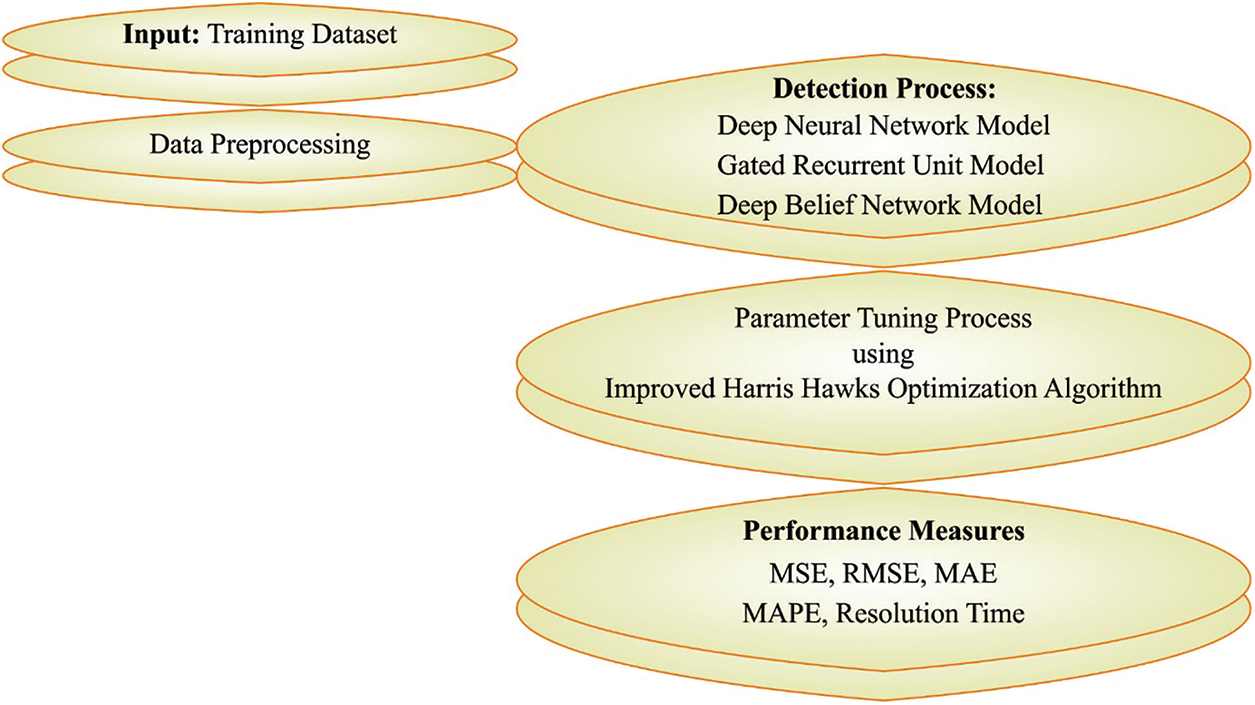
Figure 1: Overall process of IHHODL-ECP system

3.1 Normalization Process

Initially, the raw power data must be preprocessed to be compatible with further processing. The size of the original data set is distinct between power factor with demand, current, and voltage. The power factor has a number between 0 (minimum) and 1 (highest) (maximum). However, the scales for the current, demand, and voltage have a broad range. The managed value is scaled to a comparable range for each attribute and centralised to achieve a standard deviation of 1 and a mean of 0 after the standard transformation.

3.2 Fusion Based Prediction Process

For prediction process, a fusion of three DL models namely DNN, GRU, and DBN is employed for the predictive process.

3.2.1 DNN Model

Theoretically, DNN might serve as an extension of MLP-NN by incorporating several hidden layers [18]. To solve the issue of the MLP-NN gradient vanishing, in addition to this hidden layer, it uses a variety of gradient descent optimizers and a broad collection of activation functions. The gradient vanishing problem arose when the gradient of error during the training stage went smaller, but the BP model did not make any adjustments to attain the global minimums. This caused the gradient to vanish. We decided to construct a DNN mechanism for recognising human activity in medical applications using sparser data signals supplied by passive sensors, and the DNN technique was the one that we chose to use because of the benefits that it offers. It is made up of four dense layers, as well as input and output layers, both of which are hidden. A dropout layer with a ratio of 0.01 is placed on top of each veiled layer that comes after it. The next step is to add a Dropout layer to the model in order to assist it in eliminating over-fitting concerns, which can occur when there is less data from passive sensors. It is required to create the model a little bit deeper and lighter in order to arrive to a better conclusion, therefore the number of hidden units is then set to three. This is done because it is necessary to make the model more complex. DNN made use of a wide variety of activation functions, which varied according on the specific applications and utilisation conditions. Within the framework of the proposed model, the Rectified Linear Unit, or ReLU, is used as the activation function.:

f(x)=max(O,x)(1)

For the output layer, a softmax function is utilized to regularize the output value within [0, 1] where the sum of the value is equivalent to 1 as follows:

σ(n)i=eni∑l=1Lenl for i=1…L(2)

In Eq. (2), the n value in a vector of length L is regularized with exponential function. Beforehand testing and training, a pre-processing setup of the data feature for the passive sensor is implemented by means of the normalization model and normalizes the value of data feature through mean and unit variance. The normalization of data features for presented DNN method was highly significant for making the value that has dissimilar scales contribute equally resolving the bias issue in model training. In such cases, for every instance x in the data, it is normalized as follows:

z=(x−m)/s(3)

In Eq. (3), s and m indicate the standard deviation and mean of the data sample.

3.2.2 GRU Model

To conquer the gradient vanishing problems, GRU was developed by Cho. GRU is regarded as an LSTM unit without output gate [19]. The LSTM and GRU achieve excellent accuracies and have an equivalent structure. With that regard, GRU has updated and rest gates. This gate enables GRU for passing the data forward over several time windows for good classification or prediction. Especially, weights and data are stored in memory to be utilized with a provided state to upgrade the value. From the above mentioned, the GRU comprises two gates, namely update and the reset gates (present and last memory content). In update gate, GRU computes zt at a time t to resolve gradient vanishing problems as follows:

zt=σ(Wz[ht−1,xt]+bz)(4)

In the reset gate, GRU calculates zt at a time t to characterize what amount of the previous data to be forgotten:

rt=σ(Wr[ht−1,xt]+br)(5)

Present memory content phase is evaluated as follows:

h~t=tanh(Wh[rtht−1,xt])(6)

Finally, the last memory at present time step computes ht for storing the existing unit data to compute the output vector 0t as:

ht=(1−zt)ht−1+zth~(7)

ot=σo(Woht+bo)(8)

whereas bo and Wo denotes the bias and weight matrix of output layer.

3.3 DBN Model

DBN is a learning method using probability for generating the output. The framework of the DBN comprises various restricted Boltzmann machine (RBM) elements that are connected to one another [20]. The primary RBM unit was the visible layer, and the following ones were the hidden layers. Fig. 2 depicts the structure of DBN.

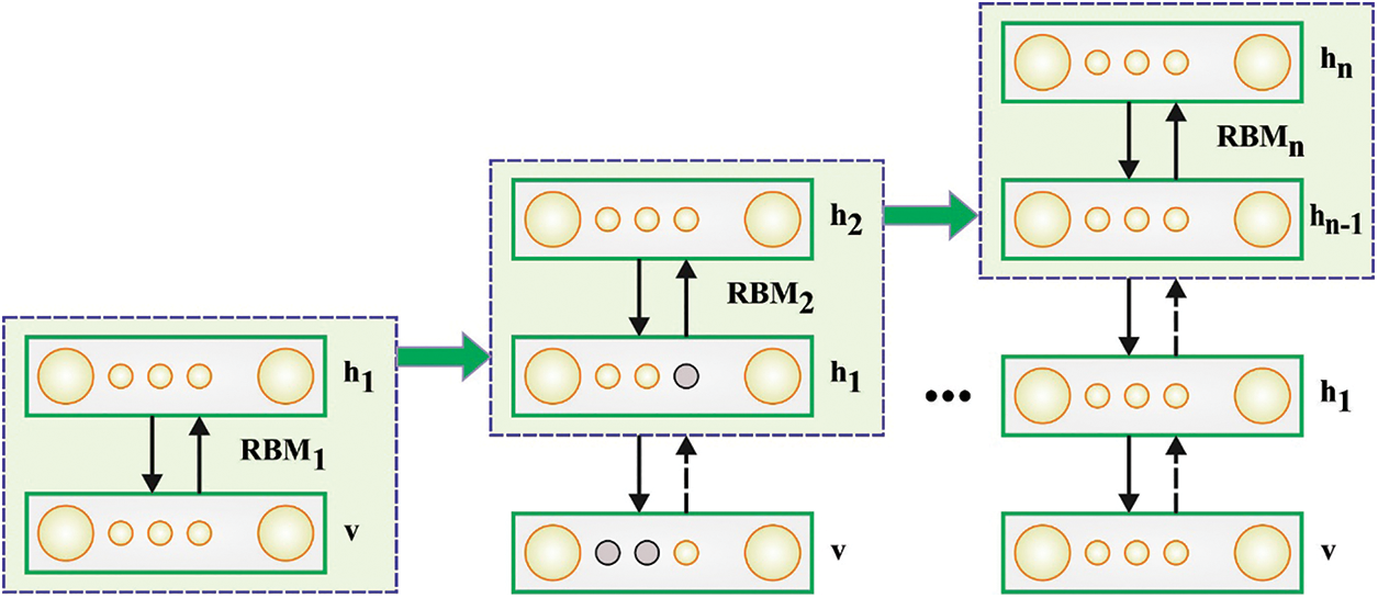
Figure 2: Framework of DBN

The framework of RBM has one hidden-and-visible layer. The neurons lie in the 2 layers were fully connected. But there was no connection among neurons in a similar layer. hi is the unit in the hidden layer h and vi labels the unit in the visible layer v. W is the connection weight among 2 layers, bi represents the bias of the hidden unit and ai indicates the offset vector of the visible unit.

3.4 Hyperparameter Tuning Process

In the final stage, the IHHO algorithm is exploited as a hyperparameter tuning strategy. HHO is a metaheuristic approach derived from Harris hawk’s predation action. The exploration stage of HHO approach is global search process [21–23]. Once hawk finds the target prey in the air, every individual coordinates the activity to discover a promising location around the prey and form siege. Initially, the Hawk appears in a specific location belongs to search space based on the randomness principle, then gradually move towards the optimum solution. Set q as a random integer positioned amongst [0, 1], if q<0.5, every individual takes movement by reference the location of prey and another one. If q≥0.5, then Harris hawk stays in a tree that is in the scope of activity of population:

X(t+1)={Xrand(t)−r1⋅|Xrand(t)−2⋅r2⋅X(t)|,q≥0.5(XPrey(t)−Xm(t))−r3⋅(lb+r4⋅(ub−lb)),q<0.5(9)

Xm=1N∑i=1NXi(t)(10)

From the expression, X(t) denotes location of population afterward tth round of iteration. Xrand shows the position of random individuals in population. XPrey indicates the location of optimum solution, Xm is the average position of population. r1,r2,r3, and r4 show the random value within [0, 1]. N indicates population size, Ub, and lb indicates the upper and lower boundaries of the problem correspondingly.

The exploitation stage is a procedure of local search. Once the prey is surrounded, the hawks take attack. The HHO simulates escaping behavior of prey and hunting strategies of hawks via distinct integration of escape energy factor E and random number ∈(0,1). r demonstrates escape probability for prey. r<0.5 implies a successful escape, but r≥0.5 symbolizes escape is not successful.

Soft besiege: If |E|≥0.5 and r≥0.5, prey is energetic and attempts to escape through jump, but ultimately it gets caught, mathematically expressed in the following:

X(t+1)=ΔX(t)−E⋅|J⋅XPrey(t)−X(t)|(11)

ΔX(t)=XPrey(t)−X(t)(12)

J=2⋅(1−r5)(13)

Here, ΔX(t) signifies the distance between optimum solution and present individual after the tth time of iteration, r5 denotes a random integer within [0, 1]. J indicates the jumping distance of prey during running for life.

Hard besiege: If |E|<0.5 and r≥0.5, prey is lack physical strength and is captured directly, equation can be given below:

X(t+1)=XPrey(t)−E⋅|ΔX(t)|(14)

Soft besiege with progressive quick dives: If |E|≥0.5 and r<0.5, prey is energetic and has probability to escape, hawk makes a further intelligent soft encirclement, then the implementation is given below:

Y=XPrey(t)−E⋅|J⋅XPrey(t)−X(t)|(15)

Z=Y+S×LF(D)(16)

X(t+1)={Y,f(Y)<f(X(t))Z,f(Z)<f(X(t))(17)

From the expression, D denotes the dimension of problem, S indicates the D dimension random vector, and LF epitomizes the Levy flight function:

LF(x)=0.01×ru×σ|rv|1β(18)

σ=(Γ(1+β)×sin⁡(πβ2)Γ(1+β2)×β×2(β−12)11β)(19)

Now, ru and rv indicate the arbitrary number amongst [0, 1], β denotes constant set to 1.5.

Hard besiege with progressive quick dives: If |E|<0.5 and r<0.5, prey has inadequate physical energy, however, it still has a possibility to escape. To decrease the average distance from prey, hawk forms the novel hard encirclement, the strategy is given below:

Y=XPrey(t)−E⋅|J⋅XPrey(t)−Xm(t)|(20)

Z=Y+S×LF(D)(21)

X(t+1)={Y,f(Y)<f(X(t))Z,f(Z)<f(X(t))(22)

The HHO control the transformation among global and local search via the escape energy factor E, that is described by the following equation:

E=2⋅E0⋅(1−tT)(23)

Let T be the maximal round of iterations, Eo as (−1,1) shows the primary value of the energy in iteration. If |E|≥1, the HHO enter into the exploration stage that characterizes individual in population move to the prey within search space. If |E|<1, search transforms into the exploitation stage.

The IHHO algorithm is derived by the Quasi-oppositional-based learning (quasi-OBL) system, which is a well-known enhancing method for boosting the convergence rate and precision of the optimized methods by making certain development to them, which was executed through comparison of search agents with their opposite number and considering the superior one as the solution agent. The quasi-opposite of X is computed below.

Xg=r and(Xg¯,BL,g+BU,g2)(24)

whereas Xˇg denotes the quasi-opposite of Xg.BU,g and BL,g were the lower and upper boundaries belonging to the search space where X can be placed with D dimensions. Xg¯ was the opposite of Xg, which was computed as follows. Xˇ is an integer arbitrarily selected, seen in the above equation,

from the range of Xg¯.

Xg¯=BU,g+BL,g−Xg(25)

g=1,2,…,D

The IHHO method will derive the main function related to mean square error (MSE) and it was employed for predicting the testing output of the DL method. It is defined below.

MSE=∑Ni|yi−y^i|2N(26)

whereas y represents the number of rounds, yi designates the experimental value, y^i signifies the forecasted values.

4  Results and Discussion

In this part, the IHHODL-ECP model’s energy consumption forecast findings are examined in depth. The IHHODL-ECP method’s actual vs. expected energy consumption is presented in Table 1 and Fig. 3. The results demonstrated that the IHHODL-ECP approach successfully predicted the values at all timestamps. The IHHODL-ECP model has achieved the projected value of 1.553 with 1 timestamp and real value of 1.465. In the meanwhile, the IHHODL-ECP technique has reached the projected value of 3.643 with a 10 timestamp and real value of 3.722. Eventually, with a timestamp of 90 and an actual value of 1.465, the IHHODL-ECP method reaches the predicted value of 1.508. Table 2 displays the overall predictive performance of the IHHODL-ECP model over five separate runs. Fig. 4 depicts an MSE and RMSE analysis of the IHHODL-ECP technique for five runs. The results revealed that the IHHODL-ECP approach lowered MSE and RMSE values. On run-1, for instance, the IHHODL-ECP approach yielded MSE values of 0.2728 and RMSE values of 0.5223. In addition, the IHHODL-ECP approach achieved MSE of 0.3369 and RMSE of 0.5804 on its third run. The IHHODL-ECP method achieved MSE of 0.2767 and RMSE of 0.5260 on run 5.

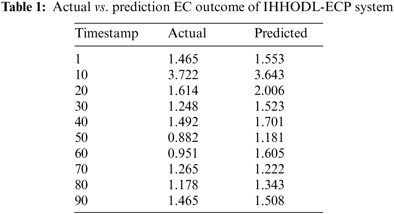
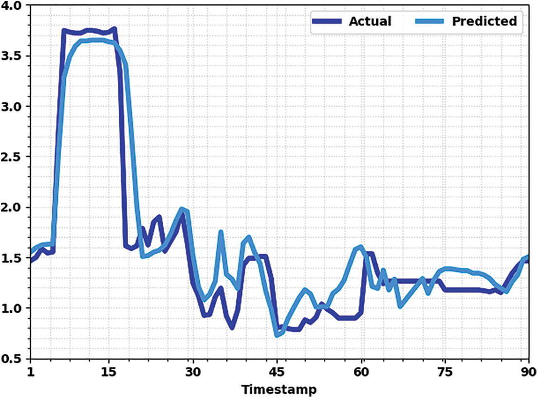
Figure 3: Actual vs. prediction EC outcome of IHHODL-ECP system

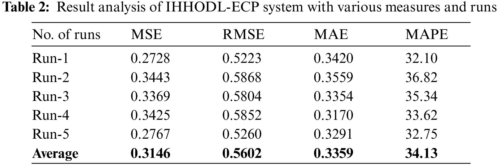
Figure 4: MSE and RMSE analysis of IHHODL-ECP system with distinct runs

Fig. 5 exhibits a MAE examination of the IHHODL-ECP method under five runs. The results show the IHHODL-ECP algorithm has resulted to reduced value of MAE. For example, on run-1, the IHHODL-ECP methodology has attained MAE of 0.3420. Moreover, on run-3, the IHHODL-ECP technique has acquired MAE of 0.3351. Subsequent, on run-5, the IHHODL-ECP model has obtained MAE of 0.3291.

Figure 5: MAE analysis of IHHODL-ECP system with distinct runs

Next, Fig. 6 displays a MAPE examination of the IHHODL-ECP method under five runs. The results demonstrated that the IHHODL-ECP algorithm has resulted to reduced value of MAPE. For example, on run-1, the IHHODL-ECP approach has gained MAPE of 32.10. Moreover, on run-3, the IHHODL-ECP technique has achieved MAPE of 35.34. Next, on run-5, the IHHODL-ECP method has attained MAPE of 32.75.

Figure 6: MAPE analysis of IHHODL-ECP system with distinct runs

Table 3 shows comparative forecasting results of the IHHODL-ECP methodology with recent models. The simulation values noticed the attention LSTM method has shown poor prediction results while the LSTM, GRU, and BiLSTM models have reached moderately closer prediction performance. Next, the CNN-LSTM model has resulted to reasonable prediction performance with MSE of 0.3708, RMSE of 0.6089, MAE of 0.3733, and MAPE of 34.77. At last, the IHHODL-ECP model has shown maximum outcome with least MSE of 0.3146, RMSE of 0.5602, MAE of 0.3359, and MAPE of 34.13.

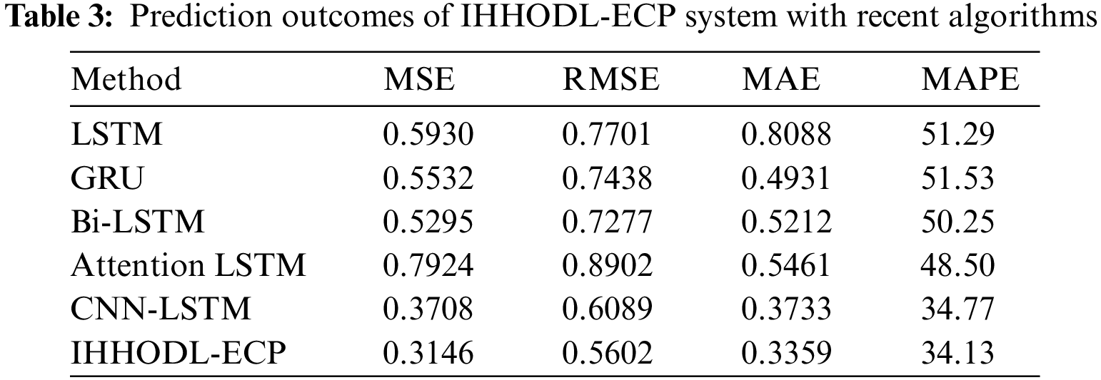
Table 4 renders a brief comparison study of the IHHODL-ECP method under distinct time resolutions. Fig. 7 exhibits a MSE study of the IHHODL-ECP approach with recent methodologies. The results exhibited the IHHODL-ECP method has resulted to least MSE values under every resolution. For instance, with minutely resolution, the IHHODL-ECP model has obtained lower MSE of 0.3146 whereas the LR, LSTM, and CNN-LSTM models have attained higher MSE of 0.5896, 0.5930, and 0.3708 correspondingly. Besides, with hourly resolution, the IHHODL-ECP methodology has accomplished lower MSE of 0.3241 whereas the LR, LSTM, and CNN-LSTM approaches have reached higher MSE of 0.4787, 0.3955, and 0.3339 correspondingly.

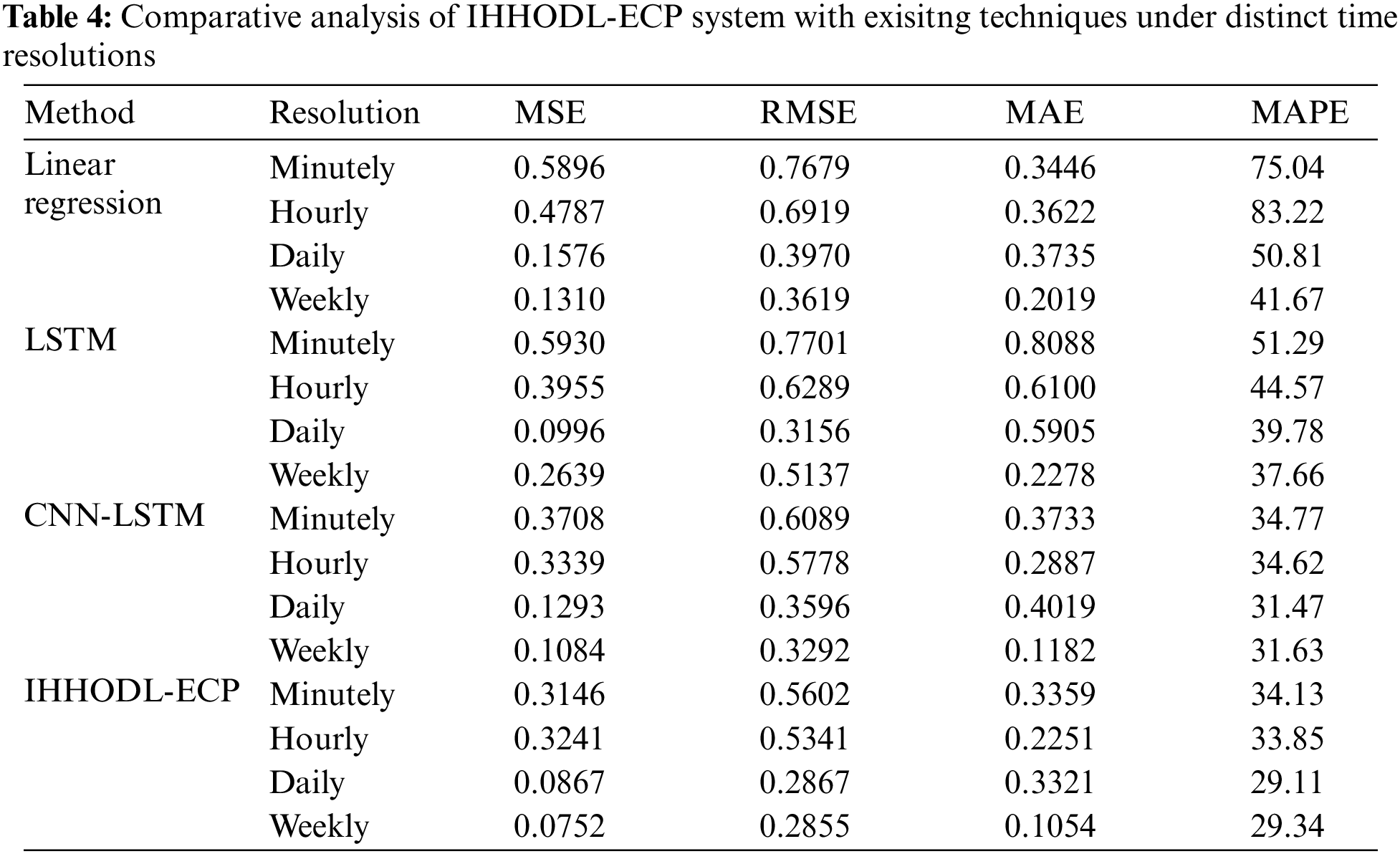
Figure 7: MSE analysis of IHHODL-ECP system under distinct time resolutions

Fig. 8 shows a RMSE investigation of the IHHODL-ECP approach with current algorithms. The outcomes exhibited the IHHODL-ECP method has least RMSE values in every resolution. For example, with minutely resolution, the IHHODL-ECP method has reached lower RMSE of 0.5602 while the LR, LSTM, and CNN-LSTM methodologies have attained maximal RMSE of 0.7679, 0.7701, and 0.6089 correspondingly. Furthermore, with hourly resolution, the IHHODL-ECP approach has acquired lower RMSE of 0.5341 while the LR, LSTM, and CNN-LSTM methodologies have achieved maximal RMSE of 0.6919, 0.6289, and 0.5778 correspondingly.

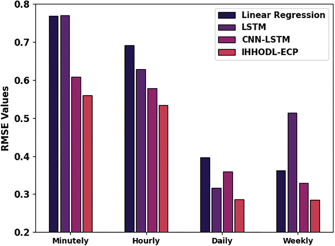
Figure 8: RMSE analysis of IHHODL-ECP system under distinct time resolutions

Fig. 9 shows a MAE analysis of the IHHODL-ECP method with current methods. The results specified the IHHODL-ECP method has resulted to least MAE values under every resolution. For example, with minutely resolution, the IHHODL-ECP model has obtained lower MAE of 0.3359 whereas the LR, LSTM, and CNN-LSTM models have attained higher MAE of 0.3446, 0.8088, and 0.3733 correspondingly. Additionally, with hourly resolution, the IHHODL-ECP model has obtained lower MAE of 0.2251 whereas the LR, LSTM, and CNN-LSTM methodologies have acquired higher MAE of 0.3622, 0.6100, and 0.2887 correspondingly.

Figure 9: MAE analysis of IHHODL-ECP system under distinct time resolutions

Fig. 10 exhibits a MAPE investigation of the IHHODL-ECP method with recent methodologies. The results designated the IHHODL-ECP method has resulted to least MAPE values under every resolution. For example, with minutely resolution, the IHHODL-ECP model has lower MAPE of 0.34.13 while the LR, LSTM, and CNN-LSTM models have attained higher MAPE of 75.04, 51.29, and 34.77 correspondingly. Besides, with hourly resolution, the IHHODL-ECP model has obtained lower MAPE of 33.85 whereas the LR, LSTM, and CNN-LSTM models have achieved higher MAPE of 83.22, 44.57, and 34.62 correspondingly. These results demonstrated the enhanced forecasting results of the IHHODL-ECP model.

Figure 10: MAPE analysis of IHHODL-ECP system under distinct time resolutions

5  Conclusion

As part of this research project, we came up with a brand-new IHHODL-ECP model to serve as a predictive instrument that can estimate integrated energy use in an Internet of Things context. For the IHHODL-ECP model that has been described, the raw data on electricity has to be preprocessed in order to make it compatible with the subsequent processing steps. A combination of three DL models, namely DNN, GRU, and DBN, is used for the predictive process. This combination is used for the prediction process. In addition to that, the IHHO method is utilised in the context of a hyperparameter tuning approach. The experimental result analysis of the IHHODL-ECP model is carried out under a variety of different aspects, and the comparative research reported the enhancements of the IHHODL-ECP model in comparison to other current algorithms. Selecting predominant feature which give more accuracy in predicting the output is identified as a limitation of this approach. In the future, the model that was shown can be extended to include the design of an ideal approach for selecting features. There is no conflicts of interest to report regarding the present study.

Funding Statement: The authors received no specific funding for this study.

Conflicts of Interest: The authors declare that they have no conflicts of interest to report regarding the present study.

References

1. S. Venkatesan, J. Lim, H. Ko and Y. Cho, “A machine learning based model for energy usage peak prediction in smart farms,” Electronics, vol. 11, no. 2, pp. 218–236, 2022. [Google Scholar]

2. W. Li, Y. Chai, F. Khan, S. R. U. Jan, S. Verma et al., “A comprehensive survey on machine learning-based big data analytics for IoT-enabled smart healthcare systems,” Mobile Networks and Applications, vol. 26, no. 1, pp. 234–252, 2021. [Google Scholar]

3. S. H. Lee, T. Lee, S. Kim and S. Park, “Energy consumption prediction system based on deep learning with edge computing,” in In proc. of 2019 IEEE 2nd Int. Conf. on Electronics Technology (ICET), Chengdu, China, pp. 473–477, 2019. [Google Scholar]

4. A. Dhillon, A. Singh, H. Vohra, C. Ellis, B. Varghese et al., “IoTPulse: Machine learning-based enterprise health information system to predict alcohol addiction in Punjab (India) using IoT and fog computing,” Enterprise Information Systems, vol. 16, no. 7, pp. 1–23, 2021. [Google Scholar]

5. T. Reddy, S. P. Rm, M. Parimala, C. L. Chowdhary, S. Hakak et al., “A deep neural networks based model for uninterrupted marine environment monitoring,” Computer Communications, vol. 157, no. 3, pp. 64–75, 2020. [Google Scholar]

6. M. Zekic-Susac, S. Mitrovic and A. Has, “Machine learning based system for managing energy efficiency of public sector as an approach towards smart cities,” International Journal of Information Management, vol. 58, pp. 1–15, 2021. [Google Scholar]

7. M. Ateeq, F. Ishmanov, M. K. Afzal and M. Naeem, “Multi-parametric analysis of reliability and energy consumption in IoT: A deep learning approach,” Sensors, vol. 19, no. 2, pp. 309–322, 2019. [Google Scholar] [PubMed]

8. O. Said and A. Tolba, “Accurate performance prediction of IoT communication systems for smart cities: An efficient deep learning based solution,” Sustainable Cities and Society, vol. 69, no. 6, pp. 1–22, 2021. [Google Scholar]

9. T. M. Ghazal, “Energy demand forecasting using fused machine learning approaches,” Intelligent Automation & Soft Computing, vol. 31, no. 1, pp. 539–553, 2022. [Google Scholar]

10. L. Sehovac, C. Nesen and K. Grolinger, “Forecasting building energy consumption with deep learning: A sequence to sequence approach,” in In proc. 2019 IEEE Int. Congress on Internet of Things (ICIOT), Milan, Italy, pp. 108–116, 2019. [Google Scholar]

11. K. Yan, X. Zhou and J. Chen, “Collaborative deep learning framework on IoT data with bidirectional NLSTM neural networks for energy consumption forecasting,” Journal of Parallel and Distributed Computing, vol. 163, no. 8, pp. 248–255, 2022. [Google Scholar]

12. H. A. Ounifi, A. Gherbi and N. Kara, “Deep machine learning-based power usage effectiveness prediction for sustainable cloud infrastructures,” Sustainable Energy Technologies and Assessments, vol. 52, no. 7, pp. 1–18, 2022. [Google Scholar]

13. N. Iqbal and D. H. Kim, “IoT task management mechanism based on predictive optimization for efficient energy consumption in smart residential buildings,” Energy and Buildings, vol. 257, pp. 1–11, 2022. [Google Scholar]

14. T. Huybrechts, P. Reiter, S. Mercelis, J. Famaey, S. Latre et al., “Automated testbench for hybrid machine learning-based worst-case energy consumption analysis on batteryless IoT devices,” Energies, vol. 14, no. 13, pp. 3914–3937, 2021. [Google Scholar]

15. T. Han, K. Muhammad, T. Hussain, J. Lloret and S. W. Baik, “An efficient deep learning framework for intelligent energy management in IoT networks,” IEEE Internet of Things Journal, vol. 8, no. 5, pp. 3170–3179, 2020. [Google Scholar]

16. M. Elsisi, M. Q. Tran, K. Mahmoud, M. Lehtonen and M. M. Darwish, “Deep learning-based industry 4.0 and internet of things towards effective energy management for smart buildings,” Sensors, vol. 21, no. 4, pp. 1038–1054, 2021. [Google Scholar] [PubMed]

17. R. Zhao, X. Wang, J. Xia and L. Fan, “Deep reinforcement learning based mobile edge computing for intelligent Internet of Things,” Physical Communication, vol. 43, no. 9, pp. 1–22, 2020. [Google Scholar]

18. Y. L. Cheng and M. H. Lim, “Impact of internet of things paradigm towards energy consumption prediction: A systematic literature review,” Sustainable Cities and Society, vol. 78, pp. 1–22, 2021. [Google Scholar]

19. C. Huang, G. Xu, S. Chen, W. Zhou, E. Y. Ng et al., “An improved federated learning approach enhanced internet of health things framework for private decentralized distributed data,” Information Sciences, vol. 614, no. 15, pp. 138–152, 2022. [Google Scholar]

20. M. M. Hassan, S. Ullah, M. S. Hossain and A. Alelaiwi, “An end-to-end deep learning model for human activity recognition from highly sparse body sensor data in internet of medical things environment,” The Journal of Supercomputing, vol. 77, no. 3, pp. 2237–2250, 2021. [Google Scholar]

21. A. Gumaei, M. M. Hassan, A. Alelaiwi and H. Alsalman, “A hybrid deep learning model for human activity recognition using multimodal body sensing data,” IEEE Access, vol. 7, pp. 99152–99160, 2019. [Google Scholar]

22. T. T. Nguyen, P. T. Tung, N. N. Tan, N. N. Linh and T. T. Luc, “A study of factors affecting GPR signal amplitudes in reinforced structures using deep belief networks,” Infrastructures, vol. 7, no. 9, pp. 123–143, 2022. [Google Scholar]

23. C. Zhu, Y. Zhang, X. Pan, W. Chen and Q. Fu, “Improved harris hawks optimization algorithm based on quantum correction and nelder-mead simplex method,” Mathematical Biosciences and Engineering, vol. 19, no. 8, pp. 7606–7648, 2022. [Google Scholar] [PubMed]