Classifying Hematoxylin and Eosin Images Using a Super-Resolution Segmentor and a Deep Ensemble Classifier

1  Introduction

Nowadays, scientists and researchers used the ML and DL models in several applications including agriculture, environment, text sentiment analyses, cyber security, and medicine [1]. Early detection of liver tumors is one of the hot research subjects in the literature since it is the sixth most common malignancy and the fourth-highest leading cause of fatalities around the world [2]. It is expected that, by 2025, around one million lives will be suffered from liver cancer [3]. Many sociodemographic features such as sex, age, and geographical region are strongly associated with liver cancer. The malignant cells in the liver can enchain together to create cancer and then spread to other tissues and organs (e.g., bones, lungs, etc.). Hepatocellular Carcinoma (HCC) is an extremely aggressive primary cancer and accounts for 90% of the cases worldwide [4]. Hence, early diagnosis of HCC is certainly imperative and requires to be carried out accurately.

Manual HCC diagnosis and segmentation of the nuclei regions in H&E stained histopathology images is a time-consuming and challenging process. Moreover, the accuracy of the manual diagnostic system is dependent on the complexity of the disease and the pathologist’s diagnostic knowledge [5], which eventually leads to an imprecise assessment. As morphological attributes of H&E stains are very complex the study of these images is very difficult and it is still in the exploratory phase in the application of clinical pathology. At the same time, these challenging factors motivated several investigators to develop novel diagnostic triage and testing strategies to support the early detection of liver cancer which can identify the tumor cells with greater accuracy and consequently improve clinical outcomes. Furthermore, the computer-aided diagnosis will be far faster than the manual screening.

DL-based HCC diagnostic systems have made noteworthy strides in the past decades; hence, several effective automatic diagnostic models have been established. Current advancements in DL approaches provide new opportunities for HCC identification and classification which have gained attention from research, academic and fiscal societies. DL models generally include various phases such as preprocessing, segmentation, feature extraction, and classification. The apposite preprocessing technique reduces the deviations in image quality, for example, denoising to minimize noise and artifacts in the image, enhancement technique to improve the contrast between background and region of interest [6], spatial filtering to enhance edges and boundaries by eliminating blur [7], and color normalization to reduce color variation in the image [8].

In HCC diagnosis, segmentation is a vital process that extracts the important tissues (e.g., nuclei, stroma, and lymphocyte) that have the required attributes to identify cancer cells. When a DL approach is employed to support liver cancer detection, efficient feature engineering can be implemented through medical oncologists, which makes it viable to realize improved enactment [9]. Apt attributes can be extracted by applying attribute selection approaches according to the pathologist’s knowledge, or other techniques. In classification, DL algorithms are used to categorize the segmented histopathology images based on their features. Conversely, several DL models may hamper the effectiveness of the collaboration between physicians and the system owing to the perplexing decision-making procedure [10,11]. Hence, increasing the efficiency of liver cancer detection systems with greater comprehensiveness (i.e., higher prediction accuracy and generalization against fluctuating data) is inevitable for automatic cancer detection models [12].

Of late, Deep Ensemble Learners (DEL) have been proposed in the literature that integrates more than one DL approach to provide improved classification results and better generalization performance [13]. Related to the individual DL classifiers, an ensemble model accomplished higher classification accuracy. DEL frequently chooses an optimum set of individual classifiers and then integrates them by means of a precise fusion technique such as stacking, support function fusion, and majority voting [14]. Therefore, the decision on selecting individual classifiers and assimilating them is critical. In order to achieve the best enactment, the selected classifiers should have optimal enactments as well as sufficient diversity [15]. Thus, the performance of these systems still needs substantial enhancement, and then only they can fulfill the demands of real-time diagnostic scenarios. In this work, we propose a DEL model to detect and classify liver cancer cells from H&E histopathological images with better accuracy. The major contributions of our work are four-fold.

1.    A super-resolution convolutional network is developed to segment various edges of nuclei in the H&E liver image.

2.    An efficient DEL classifier is developed with two base learners using a dropout extreme learning machine and enhanced convolutional block attention module-based residual networks. The proposed ECNet employs a voting mechanism to integrate the decisions from base learners.

3.    The proposed ECNet is implemented using two real-world liver cancer datasets including KMC and TCGA-LIHC and its performance is compared with some state-of-the-art classifiers in terms of selected performance metrics.

The rest of this paper is arranged as follows: Section 2 presents the basic concepts of DL classifiers. Section 3 analyses the relevant works about DL-based liver cancer classification techniques. In Section 4, we discuss the proposed ECNet in detail. Then the experimental setup is discussed in Section 5. The numerical fallouts are given in Section 6. Section 7 concludes this work.

2  Preliminaries of DL Classifiers

Generally, DL classifiers include five basic layers, viz. convolution, activation, pooling, fully-connected (dense), and output layers. The convolutional layer aims to learn feature maps (also called channels) from the dataset by applying different kernels (filters or feature detectors), by which their spatial relationship can be retained [16]. In this architecture, every pixel of a channel is associated with a region of adjacent pixels in the preceding unit. The new channel can be achieved by convolving the input with a trained filter and then performing a pixel-wise nonlinear transfer operation on the convolved fallouts. Each spatial location of the input disseminates the filter to create a channel. The feature value ( ηp,q,nl) at position (p, q) in the  nth channel of the lth layer is defined by Eq. (1) [17].

ηp,q,nl=ωnlTIp,ql+βnl   (1)

where ωnl is the weight vector and βnl is the bias term of the  nth kernel of the lth layer, correspondingly. The term Ip,ql is the input patch focused at (p, q) of the lth layer. ηp,q,nl represents the shared channel which is generated by the kernel ωnl . This weight disseminating technique can reduce the computational overhead and make the model simpler to train. The activation (transfer) operation adds nonlinearities to the classifier which is required for multi-layer classifiers to identify nonlinear attributes. Consider a(.) is the nonlinear transfer operation. The activation value (ap,q,nl) of convoluted attribute ηp,q,nl can be calculated using Eq. (2).

ap,q,nl=a(ηp,q,nl)   (2)

In general, hyperbolic tangent, sigmoid, and Rectified Linear Unit (ReLU) [16,17] are used as transfer functions. However, ReLU is one of the most widely used non-saturated transfer operations and it is defined as given in Eq. (3).

ap,q,nl=max(ηp,q,nl)    (3)

The subsampling (pooling) operation is employed to decrease the size of the attribute space obtained from the convolutional function. The pooling layer is generally located between two convolution layers. Every channel of a subsampling layer is coupled to its respective channel of the previous convolution unit. The pooling operation (pool(.)) of a particular channel ap,q,nl is defined by Eq. (4).

ρp,q,nl=pool(ar,s,nl),    ∀(r,s)∈Rpq  (4)

where Rpq is a local region about the point (p, q) . After stacking some convolution and subsampling blocks, DL networks consist of one (or multiple) dense layers which target to achieve higher-level attributes. These layers consider all nodes in the preceding unit and link them to each node of the current layer to produce global semantic data. However, this operation is not always required as it can be substituted by a 1 × 1 convolutional operation. The final layer of DL classifiers is an output layer. The softmax operator is frequently employed for classification. Suppose we have k number of data, the anticipated input-output correlations is defined by  {(I(k), J(k);k∈[1, 2, 3…k])} , in which I(k) is the kth input data, J(k) is its equivalent target class and O(k) is the output of the classifier. The loss function of the classifier can be computed using Eq. (5).

L=1K∑k=1K⁡l(∅; I(k),O(k))    (5)

Training DL classifiers is a global optimization problem. We can calculate the optimal system variables by minimizing the loss function.

3  Related Works

To date, diagnosis of HCC from histopathology images using DL techniques is an emerging field in the medical industry. With the advent of cutting-edge diagnostic imaging and DL techniques, early diagnosis of HCC is possible. Recently, Convolutional Neural Networks (CNN) have become the advanced tool for classifying medical images. Huang et al. proposed the Densely connected convolutional Networks (DenseNet) by adapting the skip-connection of the ResNet architecture and connecting all convolution layers [18]. For every layer in the DenseNet, the input denotes the channels of all the previous units, while its output channels are used as inputs to the subsequent units. Szegedy et al. presented a sophisticated model with an inception module to increase the width and depth of the system while keeping the same level of processing overhead [19]. Ioffe et al. proposed an improved inception network (Inception-V2) by employing batch normalization after performing a convolution operation [20].

Szegedy et al. refined the previous version of the inception network to develop the InceptionV3 module by implementing the concept of extra factorization to provide better performance [21]. But, the Inception-V3 network generates several network variables which leads to an overfitting issue and consequently increases the computational complexity. Later, Szegedy et al. along with a Google research team developed a classification model called I-ResNetV2 by integrating the concepts of InceptionV3 and ResNet models [22]. The resultant network replaces the kernel concatenation of inception with skip-connection to integrate the paybacks of the two models (i.e., making wider and deeper) while maintaining the same degree of system complexity. Ferreira et al. proved that a pre-trained I-ResNetV2 could be employed for identifying tumor cells in medical scans using transfer learning [23]. To classify medical images, Alom et al. developed the Inception Recurrent Residual Convolutional Neural Network (IRRCNN) [24]. The proposed model exploits a recurrent CNN unit connected with the inception unit. Togcar et al. introduced the BreastNet model for performing breast cancer identification [25]. The BreastNet model exploits the bilinear upsampling module to excerpt attributes from three different depths. Raza et al. proposed a unified model called MicroNet [26]. This model integrates an extra layer in the downsampling path to keep the feeble nuclei attributes which may be skipped in the max-pooling function.

Woo et al. proposed an efficient attention unit for the ResNet model, called CBAM [27]. This unit includes two consecutive components including a channel attention unit and a spatial attention unit. The intermediary channel is adaptively optimized by CBAM at each convolution layer of ResNet. The authors demonstrate that the total computational complexity of CBAM is relatively small regarding the number of variables and computation. This encourages us to implement an improved version of CBAM in our proposed classification model to classify the liver histopathological images. Dogantekin et al. proposed a classification model using a convolutional Extreme Learning Machine (ELM) to decrease the processing and storage complexity without mortifying the classification performance in classifying liver cancer [28]. This model uses five convolutional and two dense layers. The attributes of the final layer are fed as a source to the ELM classification algorithm. However, this algorithm provides better clinical outcomes when adequate hidden layers are employed. Aatresh et al. proposed an effective and reliable DL approach for automated classification of liver cancer from H&E stained liver histopathology data, called LiverNet [29]. This model uses CBAM with spatial pooling blocks for efficient liver cancer identification. Though the classification enactment of the liver cancer diagnostic system is increased through the abovementioned models, the variables and other processing overhead are still very high for simple applications. Most of the classification algorithms could effectively categorize the medical scan into benign and malicious. Even though, the segmentation algorithms used in these models provide acceptable results unraveling overlapped nuclei remains a perplexing task. To the best of our knowledge, our ECNet is among the first deep ensemble learner to develop a robust classification approach for HCC detection.

4  Proposed DEL-Based Liver Cancer Diagnostic System

The proposed deep ensemble diagnostic system integrates a deep segmentation algorithm to segment various contours of nuclei in H&E images and a deep ensemble classifier to detect and classify liver cancer cells from H&E stained histopathology scans. In the ECNet model, the nuclei regions in the liver image are first extracted through the super-resolution networks. Then, the segmented nuclei regions are fed into a DEL for classification. This deep ensemble classifier contains two different classifiers including the DrpXLM classifier and ECBAM-based ResNet. Fig. 1 illustrates the architecture of the proposed ECNet.

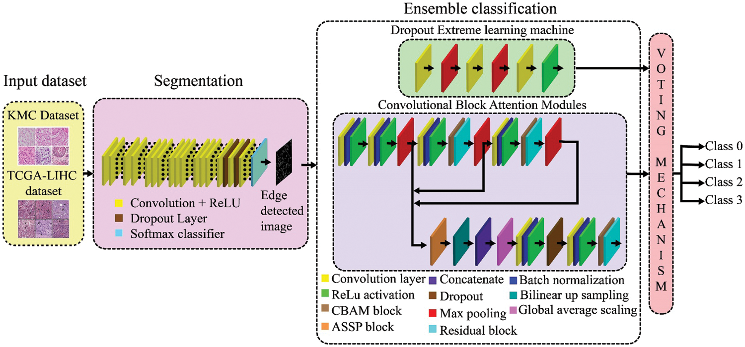
Figure 1: Architecture of ECNet for liver tumor segmentation and classification

4.1 Nuclei Segmentation Using SrCN

Nuclei segmentation is a vital process in the automatic liver cancer diagnostic system since it can extract edge information of nuclei size and shapes which possess vital attributes of liver tumor. Thus, it makes the tumor detection process easier and minimizes its processing overhead significantly. Our SrCN is a high resolution-preserving DL approach to produce very accurate segmentation. In this network, the RGB (histopathology) images are given as input for extracting the nuclei. The SrCN learns higher-level attributes by relating the source scans to its analogous ground-truth binary masks with slight resolution loss. The super-resolution channels of each input pixel are preserved by eliminating each pooling layer in the SrCN network. The SrCN segmentor consists of 16 convolution layers. But, the last three Fully-Connected Layers (FCL) are replaced by the convolution layers to enable the system to create dense prediction maps with an equal dimension as the source scans. The initial layers of SrCN learn local statistics and high-level feature representations whereas the last three layers learn delicate and low-level features of nuclei edges.

In this work, we apply the color normalization technique to minimize inter-color variation in a set of input scans. We achieve color normalization by transforming color from a target scan and also improving the contrast for fade scans to some extent. In this model, boundary identification is carried out according to the measured local Standard Deviation (SD) value in an ‘ s×s ’ window (mask) about every pixel in the image. By applying the SD value, the SrCN segmentor is less sensitive to noise. The initial phase of boundary finding is to consider only ‘r’ space statistics of the color normalized scan, as it generally holds foreground statistics (i.e., nuclei), which are perceived in the entire database. When transforming the RGB scan to ‘r’ space information numerous stains are spontaneously unglued from the image. Hence, this proposed model did not use any stain isolation technique. The ‘r’ space scan is then processed with a non-linear kernel, which is the inverse logarithm of the digital Gaussian kernel in a 3 × 3 mask. This kernel decreases noise at a certain level in H&E scans. The user selects n number of input images with different microscopic zooms (such as 10×, 30×, or 40×). Then, ‘n’ is multiplied by 0.15 and kept in a parameter ‘s’. Accordingly, for 10× scans, s = 2, for 30× scans, s = 5, and for 40× scans s = 6.

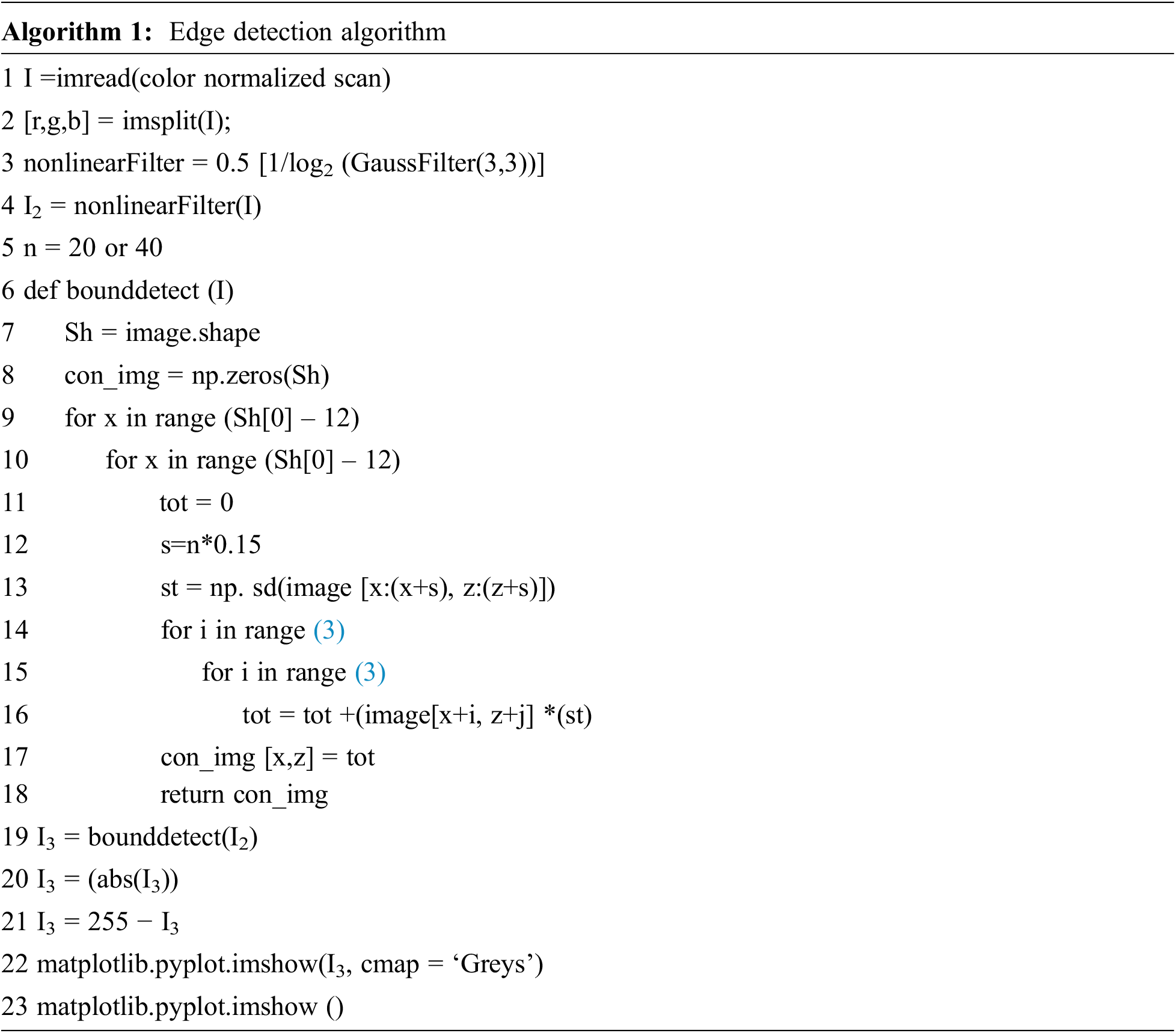
The filtered greyscale scan is further convolved with a 3 × 3 window with variable factors. Initially, we consider the SD of ‘s × s’ pixels about the first pixel in the scan, and the equal SD value is assigned in all nine variables of a 3 × 3 window. Next, the intensity of pixels (where a 3 × 3 window is being employed) is multiplied by the window factor and then we aggregate those results in a variable ‘tot’ and substitute the initial intensity of each pixel with ‘tot’, as illustrated in Algorithm 1. Subsequently, this 3 × 3 mask (window) is moved right side of the scan by one step and the process of allocating intensity values to each pixel of the scan is repeated. Fig. 2 illustrates various steps in our SrCN segmentor. The boundary of the segmented nuclei is resized into a constant dimension of 256 × 256 pixels through bi-linear interpolation for all learning, validation, and testing data. Then, our deep ensemble learner with DrpXLM and ECBAM-based ResNet classification algorithms is used for the segmented histopathology images for classification. The ensemble classifier can exploit the strong points of the base learners and can mitigate their feebleness, ultimately realizing a greater classification performance than any individual classifiers.

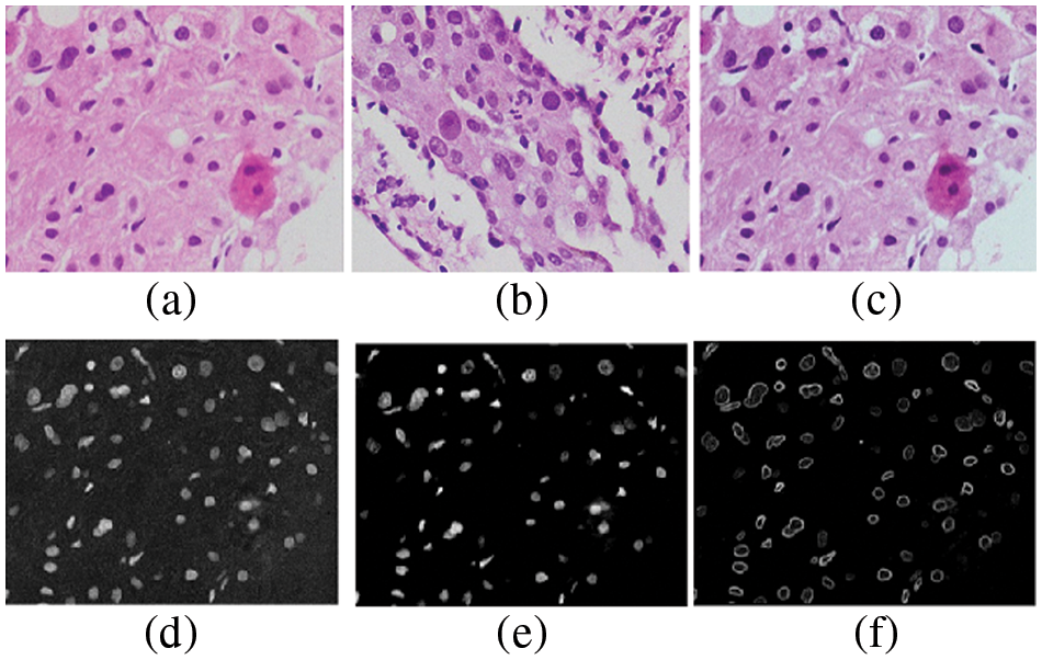
Figure 2: Edge detection (a) source scan (b) target scan (c) color normalized scan (d) color normalized scan for taking ‘r’ space information (e) ‘r’ space information after using non-linear filter (f) edge detected scan

4.2 Deep Ensemble Classification

Due to the diversity of disease types and the heterogeneity of databases, individual deep leaners are likely to limit the performance of disease detection and classification models. In line with this issue, we propose a DEL model to integrate simple and effective classifiers. Our ECNet employs two classifiers including DrpXLM and ECBAM-based ResNet classifiers. ECNet applies a voting mechanism to integrate the decisions of individual classifiers by applying the average of probabilities rule. Implementation of this integrated ensemble model with a voting mechanism can provide both better accuracy and diversity in the classification system.

4.2.1 Dropout Extreme Learning Machine

An extreme learning machine is an effective deep learner model for training Single hidden Layer Feed-forward neural Networks (SLFNs) with high speed and better generalization aptitude. In this approach, the weights and bias terms of the input and hidden layers are arbitrarily selected, whereas the hyperparameters of the output layer are systematically derived by calculating a generalized inverse matrix. Conversely, there are two important issues in ELM including the selection of structural design and the prediction variability. To address these issues, we apply the dropout method in the ELM classification model. The rudimentary concept of the dropout mechanism is to arbitrarily discard connections along with corresponding units from deep learners during the learning process, which averts their co-adaptation due to the overfitting problem. SLFN with h hidden neurons is defined using Eq. (6).

fh(x)=∑i=1h⁡Ai(xi,wi,βi)Oi     (6)

where Ai represents the activation operation; wi∈Rd is the input weight vector; βi∈R is the bias term, and Oi∈Rm is the output weight vector of the ith hidden neuron. In extreme learning, wi and βi are arbitrarily selected, whereas Oi is computed logically. The additive nodes and radial basis function neurons are frequently employed as hidden neurons. If these neurons are additive with transfer function  a(.) , then Ai is expressed as given in Eq. (7).

Ai(x,wi,βi)=a(wix+βi)   (7)

If the hidden neurons are radial basis function nodes with transfer function  a(.) , then Ai is expressed as given in Eq. (8).

Ai(x,wi,βi)=a(βi||x−wi||)   (8)

Given a training dataset  T={(xi,yi)|xi∈Rd|, yi∈Rk, i=1,2} , where xi is an input vector with the size of d × 1 and yi is a target vector with the size of k × 1. Since Ai(x,wi,βi) in Eq. (6) defines a similar transfer operation, we assume  Ai(xi,wi,βi)=A(x, w,β) , and replace xi and yi by x and fh(x) in Eq. (6), correspondingly, to get the following Eq. (9).

yi=∑j=1h⁡Ai(xi,wj,βj)Oi (9)

where  i=1,2,3…h . Eq. (9) can be inscribed in a more compact form as given in Eq. (10).

GO=Y     (10)

where

G=[A(x1,w1,β1)…A(x1,wh,βh)...……A(xn,w1,β1)…A(xn,wh,βh)] ,  O=(O1T,O2T,…OhT)T, and  Y=(Y1T,Y2T,…YhT)T

G is the output matrix of the hidden layer, where ith column of G is the ith output vector of hidden nodes relating to inputs x1,x2,…xn , and the ith row of G is the output vector of the hidden layer relating to input xi . If the number of hidden neurons is the same as the number of individual learning data samples, the matrix G is square and invertible, and SLFN can estimate these learning datasets with zero error. However, in most cases, the number of hidden neurons is considerably smaller than the number of learning datasets. Consequently, G is a non-square matrix and we cannot find an optimal solution to the system. However, we can determine its optimal (smallest norm least-squares) solution by resolving the objective function given in Eq. (11).

minβ||GO−Y|| (11)

The optimal solution of Eq. (11) can be calculated by Eq. (12).

O^=G‡Y  (12)

where G‡=(GGT)−1G is the Moore-Penrose generalized inverse of matrix  G . In this work, we implement the dropout method in the original ELM classifier to address the overfitting problem. The dropout mechanism arbitrarily discards units in consort with their links from deep models during learning. This technique averts the co-adaptation issue due to the overfitting problem in the dataset. Given an input vector  I={I1,I2, …In} , the output of linear node  n(I) is defined using Eq. (13).

γ(I)=∑i=1n⁡wiIi      (13)

If we drop Ii (1≤i≤n) with a uniform distribution or drop Ii (1≤i≤n) with a likelihood of 12 . Consequently, we get 2n subnets with the empty network. The average of outputs of the 2n subnets is calculated using Eq. (14).

Oavg(γ)=12n∑N⁡γ(N,I) (14)

where N is the set of all subnets. The term αi (1≤i≤n) represents n Bernoulli arbitrary variables and  ri=R(αi=1) ,  si=S(αi=0) . If we drop Ii (1≤i≤n) or wi (1≤i≤n) with a likelihood of si then, the output of the linear node is calculated by Eq. (15).

γ(I)=∑i=1n⁡wiαi Ii (15)

Now, we can calculate the mathematical expectation of the output of linear neurons using Eq. (16).

E(γ)=∑i=1n⁡wiE(αi) Ii=∑i=1n⁡wiri Ii (16)

If r1=r2=…rn=r , then formula (16) becomes the following Eq. (17).

E(γ)=∑i=1n⁡wiE(α) Ii=∑i=1n⁡wir Ii (17)

If there is a bias term β in the linear node, then the output of the linear node can be defined as Eq. (18).

γ(I)=∑i=1n⁡wir Ii+βrβ  (18)

In the above equation,  rβ=P(αβ=1) .

4.2.2 Enhanced CBAM-Based ResNet Classifier

Woo et al. introduced the idea of CBAM [27]. The authors exploit sequential channel attention and spatial attention units to provide attention maps that can be multiplied against the input channel. They also proved that the CBAM can enhance prediction accuracy when it is incorporated into advanced classifiers. The CBAM-based deep classifiers pay attention to the region of interest in the network. Given an intermediate channel ℱ∈RW×D×C is given as an input to the CBAM at an intermediary point in terms of depth (D), width (W), and cardinality (C) in the encoder pipeline. CBAM successively deduces a 1D channel attention map 𝒜c∈R1×1×C and a 2D spatial attention map  𝒜s∈RW×D×1 . The entire attention task can be defined as given in (19).

⟨ℱ′=𝒜c(ℱ)⊛Fℱ′′=𝒜c(ℱ′)⊛ℱ′ (19)

where ⊛ represents component-wise multiplication. ℱ′ is the intermediary result following the component-wise multiplication between the 𝒜c∈R1×1×C and ℱ . The term ℱ′′ is the ultimate result of the attention unit, and also the product of component-wise multiplication between  𝒜s∈RW×D×1 and ℱ′ . We create 𝒜c using the inter-channel correlation between attributes. The channel attention block utilizes both max-pooling and average-pooling results with a shared dense network. First, we integrate spatial statistics of a channel by applying both average pooling and max-pooling functions. We introduce two spatial context identifiers ℱavgc and  ℱmaxc to represent average- and max-pooling attributes, correspondingly. Both identifiers are then disseminated to a dense layer to generate  𝒜c∈R1×1×C . The shared network contains FCL with one hidden unit. To minimize parameter cost, the size of the hidden activation is fixed to R1×1×C/r , where  r is the reduction factor. Once the dense layer is used for every identifier, we combine the attribute vectors through component-wise addition. In brief, the channel attention is determined by Eqs. (20) and (21).

𝒜c(ℱ)=ρ(FCL(AvgPool(ℱ))+FCL(MaxPool(ℱ))) (20)

𝒜c(ℱ)=ρ(ω1(ω0(ℱavgc))+ω1(ω0( ℱmaxc)))    (21)

where ρ represents the sigmoid function, ω1∈Rc/r×c and ω0∈Rc×c/r . The FCL parameters ( ω1 and ω0 ), are disseminated for both inputs and the ReLU activation function. We create a spatial attention map using the inter-spatial correlation of attributes. On the connected attribute identifier, we implement a convolutional unit to produce  𝒜s(ℱ)∈RW×D×1 which deduces where to emphasize or quash. The residual unit employed in our ECNet model is similar to the residual unit discussed in [20] and has been implemented in [25]. The only difference being the kernels of the first convolutional unit in our residual unit is decreased by a ratio of 4 related to the kernel employed in the residual unit discussed in [25]. This not only decreased the number of system variables essential for classification but also increased the attributes gained from the input.

An atrous spatial pyramid (ASP) pooling unit can effectively gain multi-scale attributes from a channel. Considering its efficacy, we implement an identical ASP pooling block in our classifier. Atrous (dilated) convolutional operation can be employed to increase the receptive arena dimension without increasing the number of variables used. Consider an input 2D signal X convolved with a 2D kernel ω using dilated convolutional operation. This operation is defined as given in Eq. (22).

Y[i.j]=∑h⁡∑n⁡X[i+r.m, j+r.n]ω[h][n]   (22)

where r denotes the rate at which the input is sampled (i.e., dilation rate). The impact of dilation increasing the size of the receptive field of the filter is equal to appending (r – 1) zeros in between the filter components. Hence, for r = 2, a 3 × 3 filter will have a receptive field size corresponding to a 5 × 5 filter but with only nine variables. A similar idea can be applied for higher values of r = 4, 5, 6, etc. The ASP pooling unit employed in our model considers a channel as input and perform the following convolutional operations simultaneously: (i) 1 × 1; (ii) 3 × 3 with r = 2; (iii) 3 × 3 with r = 3; (iv) 3 × 3 with r = 6 (v) 3 × 3 with r = 8; and (vi) global average subsampling. Each convolutional function in each branch is performed with a batch-normalization and a ReLU transfer function. In this model, we have employed depthwise separable convolutions to decrease the number of variables and make the model more effective. This operation needs only 18 th the number of variables and only 19 th the number of iterations. The expression for depthwise separable convolutions is designated by considering an input scan I of dimension Df × Df × M and a kernel w of dimension Dk × Dk × N. The depthwise separable convolution can be performed in 2 steps: (i) depthwise convolution; and (ii) pixel-wise convolution. In the first step, the image (I) is convolved with ωD kernel with the dimension of Dk × Dk × 1.

ID=I ⊛ ωD (23)

where the dimension of ID is Dp × Dp × M. After performing this function, the pixel-wise convolutional function employs a 1 × 1 × M filter convolved with the intermediary result for each size N of the basic filter ω . This can be defined in Eq. (24).

IP=ID⊛ωP  (24)

where ωP is the filter of dimension N × 1 × 1 × M and IP is the ultimate output from the convolutional layer. The results obtained from convolutional and subsampling operations are combined and fed into a 1 × 1 convolutional unit to keep the same kernel dimension as that of the input image. This output of the convolutional layer is fed into batch normalization and ReLU transfer units before they are moved into the bilinear upsampling unit. In our classifier, we perform the ASP pooling operation after performing every max-pooling operation in the encoder block. The max-pooled output comprises higher-level attributes at various extents and scales. ASP pooling units are employed in this model to extract this data before it is upsampled and handled by the hyper-column method.

4.2.3 Voting Mechanism

The estimation of each contributing base learner in the deep ensemble method may be preserved as a vote for a particular class, i.e., normal (class 0) or malevolent (class 1, class 2, and class 3). It exploits two individual classification algorithms (i.e., DrpXLM and ECBAM-based ResNet) and implements an integration rule for making decisions. In the ECNet model, we use an average likelihoods technique to make a decision. In this model, the class label is selected based on the maximum value of the average of likelihoods. Let u represents the number of base learners C={C1, C2,….Cu} with c classes Ω={Ω1,Ω2,…Ωc} . In our experiment, we select the values c=4 and m=2 . A classifier Ci: Rn→[0,1]c accepts an input sample xi∈Rn and provides the output as a vector δci(φ1|x), δci(φ2|x),…δci(φc|x) , where δci(φk|x) denotes the likelihood assigned by Ci that input sample x fits into class  φk . The term  ALk is the average of likelihoods assigned by the classifiers for each class. It can be computed using Eq. (25).

 ALk=1m∑i=1m⁡δci(φk|x) (25)

Let AL=[al1,al2,…alc] is the set of the average of likelihoods for c classes and x is assigned to the weight φc if  ALk is having a maximum value in the set  AL .

5  Experimental Setup

The proposed ECNet classifier is realized using MATLAB 2017b Deep Learning Toolbox. The experiments are carried out on Intel® CoreTM i7-6850K CPU with 3.360 GHz 16 GB RAM and a CUDA-enabled GPU of NVIDIA GeForce GTX 1080. The effectiveness of our model is demonstrated using two real-world liver cancer datasets including KMC and TCGA-LIHC and its performance is compared with some state-of-the-art classification models in terms of evaluation metrics such as accuracy, sensitivity, specificity, precision, and JSS.

5.1 Dataset Preparation

To demonstrate the effectiveness of ECNet, we use a corpus of labeled liver tissue images from two datasets: KMC and TCGA-LIHC [26]. The KMC dataset contains 257 recently collected original liver images by pathologists from different patients. Table 1 shows the statistical report of each instance in this dataset. We apply normalization and resizing methods as data reprocessing methods to all datasets. The databases have been normalized in the range of [−1, +1] before segmentation. The normalization improves the consistency among input scans, and it delivers steady convergence. The images are resized to 224 × 224 before giving in to the classifier using bilinear interpolation. To realize a more precise evaluation of a model’s enactment, the k-fold cross-validation (CV) is used. ECNet assigns k equals 10. In a 10-fold CV, the whole database is divided into 10 parts. For each folding, one part of the dataset is used for testing and the other part is combined for training Then, we compute the average value of results across all ten autonomous trials. Indeed, a separate set of data samples for testing and validation are not presented in the database. Therefore, we have deliberately split the existing dataset into 70% for learning, 20% for testing, and 10% for validation. Furthermore, since we used 10-folds CV, the total data samples are split into 10 parts (each of 10%). Now, one fold (10%) is applied for testing, while the residual samples (90%) are split for validation and training. The utilization of 10-fold CV guarantees that each slide in the data gets to be in a test exactly once

5.2 Evaluation Measures

To evaluate the effectiveness of ECNet using the deep ensemble classifiers, we used five significant evaluation metrics including classification accuracy, sensitivity, specificity, precision, and JSS. These performance measures are required to be higher to improve the effectiveness of the proposed model. The utility is computed in terms of classification accuracy as given in Eq. (26).

Accuracy (ACC) =TN+TPTN+TP+FN+FP  (26)

where true positive (TP) signifies the number of images correctly classified as malignant; false negative (FN) represents the number of malignant images incorrectly recognized as normal. The term true negative (TN) signifies the number of images correctly classified as normal and false positive (FP) describes the number of normal images mistakenly classified as malignant ones. Sensitivity is the rate of disease detection and specificity signifies the false alarm rate.

Sensitivity (SEN)=TPTP+FN (27)

Specificity (SPE) =FPTN+FP (28)

Precision identifies the abnormal data samples that accurately belong to the malevolent class. It is computed using Eq. (29).

Precision (PRE)=TPTP+FP  (29)

JSS estimate delivers the similarity between the ground truth and the classified data. It is calculated using Eq. (30).

Jaccard similarity score (JSS)=TPTP+FN+FP     (30)

The Wilcoxon statistical test is conducted to determine whether the ECNet classifier provides a remarkable enhancement compared to other classifiers or not at a level of 5% statistical importance [28]. If the outputs of this test ρ<5 % signify that there is a significant difference at this level of significance. Otherwise there is no noteworthy difference between the related outcomes.

6  Results and Discussion

The performance of our ECNet classifier is evaluated by comparing the numerical results with that of 9 state-of-the-art classifiers, such as ResNet [20], DenseNet [18], I_ResNetV2 [23], IRRCN [24], BreastNet [25], MicroNet [26], CBAM [27], ELM [30], and LiverNet [29]. All these networks were applied, analyzed, and compared by applying the same learning, testing, and validation data samples through MATLAB 2017b DL Toolbox. The proposed classifier network is applied to the KMC and TCGA-LIHC datasets. The comprehensive results achieved by the proposed model are given in Table 2. By applying our model on KMC dataset, we can find that the ResNet model has achieved nominal enactment with 86.4% accuracy, 98.1% sensitivity, 68% specificity, 82.8% precision, and 76.5% JSS by introducing the trainable layers. The DenseNet classification model concatenates the channels while maintaining all statistics leading to motivating feature reclaim. Hence, it has generated reasonable outputs related to the ResNet classifier. The performance of DenseNet is better than ResNet in terms of accuracy (87.5%), sensitivity (98.8%), precision (84.4%), and JSS (79%) due to the capacity of DenseNet in obtaining more paradigmatic and discriminative features for more accurate segmentation.

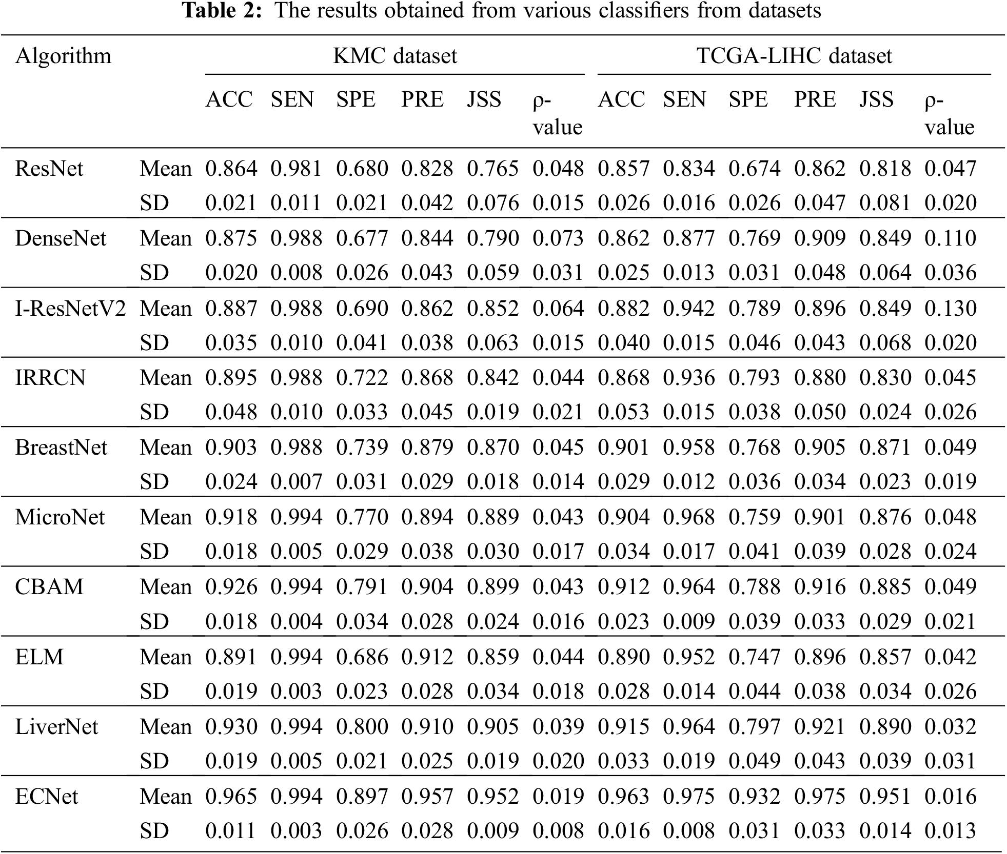
I-ResNet-v2 classifier realized better classification performance related to the other classifiers like ResNet and DenseNet. I-ResNet-v2 model substituted the kernel concatenation of inception with residual skip-connections to take the advantages of the ResNet and DenseNet models while maintaining the same level of processing overhead. It achieves 88.7% accuracy, 98.8% sensitivity, 69% specificity, 86.2% precision and 85.2% JSS. The dropout technique used in the ELM model can improve the prediction stability of the classification process. It provides a similar classification performance related to I-ResNetV2. The IRRCN model exploits the recurrent convolutional block with the inception and the residual network blocks. This model yields improved performance with an accuracy of 89.5%, sensitivity of 98.8%, specificity of 72.2%, precision of 86.8%, and JSS of 84.2%. The BreastNet exploits the bilinear upsampling layer, which enables the classifier to obtain attributes from various depths. Hence, this model achieves better results in terms of accuracy, sensitivity, specificity, precision, and JSS with 90.3%, 98.8%, 73.9%, 87.9%, and 87%, respectively. The MicroNet exploits skip-connections to assimilate lower-level attributes and efficiently combine them with multi-level attributes through a biased loss function. In terms of accuracy, sensitivity, specificity, precision, and JSS, MicroNet showed 91.8%, 99.4%, 77%, 89.4%, and 88.9%, respectively. The CBAM classifier achieves much higher classification performance with an accuracy of 92.6%, sensitivity of 99.4%, specificity of 79.1%, precision of 90.4%, and JSS of 89.9%.

The classification model using LiverNet hit better results with 93% accuracy, 99.4% sensitivity, 80% specificity, 90% precision, and 90.5% JSS. The classification performance of the proposed ensemble classifier, ECNet is usually better than the classification performance of each base learner used in ensemble systems such as DrpXLM and CBAM. As an average of 10-fold trials, the ECNet classifier achieved better results with an accuracy of 96.5%, sensitivity of 99.4%, specificity of 89.7%, precision of 95.7%, and JSS of 95.2%. The classification accuracy of the ECNet model is significantly greater by 8.35% than the individual DrpXLM classifier and slightly greater by 3.8% than the CBAM-based classifier as shown in Figs. 3 and 4. It can be witnessed that the SD of the ECNet was less than all other classifiers. Hence, the ECNet classification model delivers much more reliable outcomes for identifying liver cancer than the others. More precisely, ECNet is a very viable method for detecting liver cancer.

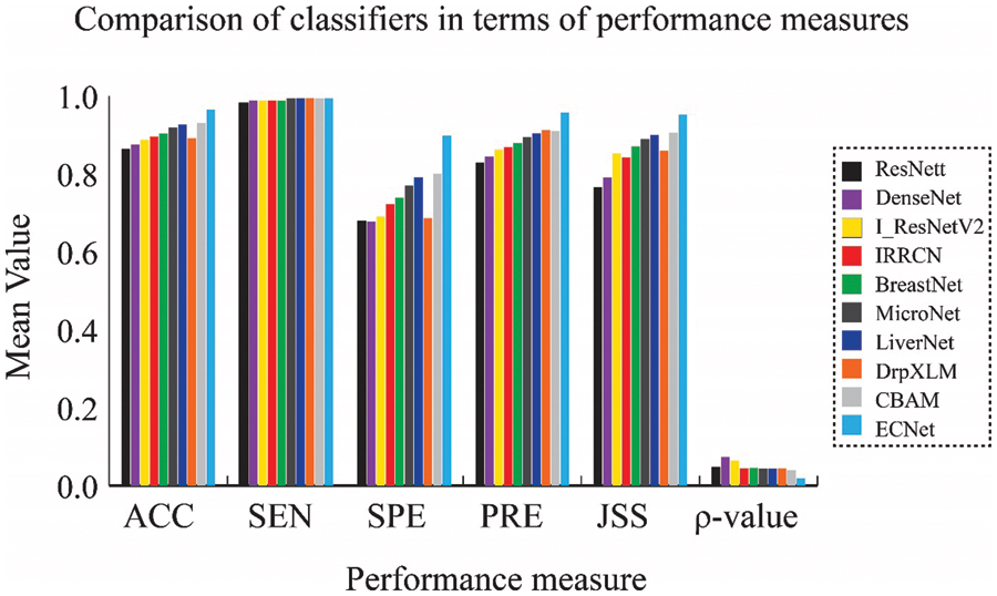
Figure 3: Comparison of results obtained from the KMC dataset in terms of the mean value of performance measures

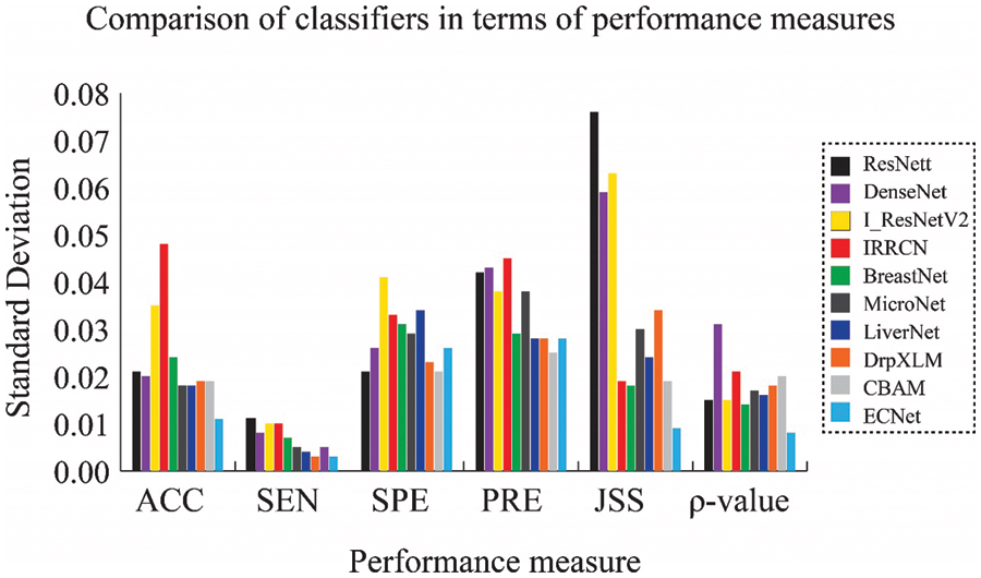
Figure 4: Comparison of results obtained from the KMC dataset in terms of SD of performance measures

We can achieve related results when we implement our model on the TCGA-LIHC liver dataset. The mean value of evaluation metrics and SD obtained from the TCGA-LIHC liver cancer dataset are given in Figs. 5 and 6. It is possible to conclude that the ECNet model has realized much-improved performance with 96.3% accuracy, 97.5% sensitivity, 93.2% specificity, 97.5% precision, and 95.1% JSS. Similarly, it is also witnessed that the SD obtained by the ECNet is lesser than that of all most all other classifiers which signify that the ECNet can yield more consistent and credible diagnosis results. Figs. 3–6 also display the Wilcoxon rank-sum test results. In most cases, it can be easily observed that the ρ values measured by the rank-sum test are less than 5% which demonstrates the superior enactment of ECNet. The proposed ECNet classifier decreases the time consumption of training and testing procedures. It consumes only 12.22 and 1.24 s, respectively in the KMC dataset. In the case of the TCGA-LIHC dataset, it takes 14.28 and 1.56 s for the training and testing process respectively. From this extensive empirical analysis, we can conclude that our ECNet is the better liver cancer diagnostic model related to state-of-the-art classifiers. However, this model does not consider the false alarm rate of the classification.

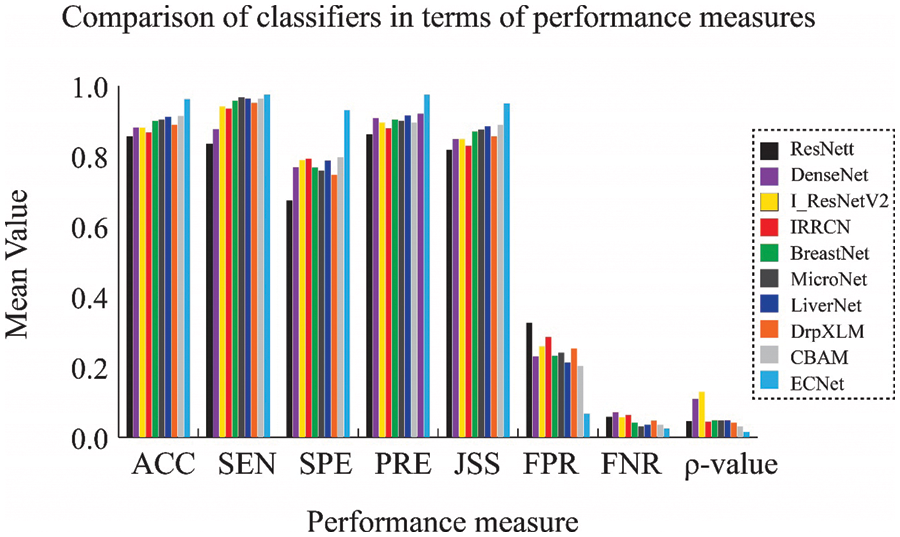
Figure 5: Comparison of results obtained from the TCGA-LIHC dataset in terms of the mean value

Figure 6: Comparison of results obtained from the TCGA-LIHC dataset in terms of the SD value

7  Conclusions

Through this work, we develop a very efficient deep ensemble classifier to categorize H&E liver histopathology images. ECNet applies a voting mechanism to integrate the decisions of individual classifiers using the average of probabilities rule. Initially, the nuclei regions in the image are segmented through SrCN, and then the segmented nuclei regions are fed into the ensemble DL network for classification. The empirical results obtained from the proposed model are related to some state-of-the-art classifiers in terms of performance metrics. The results of our meticulous experiments on the KMC liver dataset reveal that the proposed ECNet significantly outperforms other prevailing classification networks with better accuracy, sensitivity, specificity, precision, and JSS. Also, we carry out the Wilcoxon rank-sum test to determine whether the ECNet provides a considerable performance improvement or not. From extensive empirical analysis, we can conclude that our ECNet is the better liver cancer detection model related to state-of-the-art classifiers. We believe that this work will create cognition and interest in the field of liver cancer detection and related disease management. However, this work does not focus on false alarm rate and timing complexity of the intended algorithm. Moreover, the classification accuracy depends on the dataset used for experimentation. Hence, we plan to develop more generalized detection model with superior classification performance. Also, we plan to analyze the false alarm rate and timing complexity related to this proposed model in detail.

Funding Statement: The authors received no specific funding for this study.

Conflicts of Interest: The authors declare that they have no conflicts of interest to report regarding the present study.

References

1. I. H. Sarker, “Machine learning: Algorithms, real-world applications and research directions,” Springer Nature Computer Science, vol. 2, pp. 160–168, 2021. [Google Scholar]

2. H. Sung, J. Ferlay, R. L. Siegel, M. Laversanne, I. Soerjomataram et al., “Global cancer statistics 2020: GLOBOCAN estimates of incidence and mortality worldwide for 36 cancers in 185 countries,” A Cancer Journal for Clinicians, vol. 71, no. 3, pp. 209–249, 2021. [Google Scholar]

3. J. M. Llovet, R. K. Kelley, A. Villanueva, A. G. Singal, E. Pikarsky et al., “Hepatocellular carcinoma,” Nature Reviews Disease Primers, vol. 7, no. 6, pp. 321–330, 2021. [Google Scholar]

4. S. Diwakar, A. N. Srinivas and P. K. Divya, “Etiology of hepatocellular carcinoma: Special focus on fatty liver disease,” Frontiers in Oncology, vol. 10, pp. 601710, 2020. [Google Scholar]

5. A. A. Aatresh, K. Alabhya, S. Lal, J. Kini and P. U. Saxena, “LiverNet: Efficient and robust deep learning model for automatic diagnosis of sub-types of liver hepatocellular carcinoma cancer from H&E stained liver histopathology images,” International Journal of Computer Assisted Radiology and Surgery, vol. 16, no. 9, pp. 1549–1563, 2021. [Google Scholar] [PubMed]

6. C. Yao, S. Jin, M. Liu and X. Ban, “Dense residual transformer for image denoising,” Electronics, vol. 11, pp. 418, 2022. [Google Scholar]

7. S. M. Răboacă, C. Dumitrescu, C. Filote and I. Manta, “A new adaptive spatial filtering method in the wavelet domain for medical images,” Applied Sciences, vol. 10, no. 16, pp. 5693, 2020. [Google Scholar]

8. M. Z. Hoque, A. Keskinarkaus, P. Nyberg and T. Seppänen, “Retinex model based stain normalization technique for whole slide image analysis,” Computerized Medical Imaging and Graphics, vol. 90, pp. 101901, 2021. [Google Scholar] [PubMed]

9. S. J. Zhou and X. Li, “Feature engineering vs. deep learning for paper section identification: Toward applications in Chinese medical literature,” Information Processing and Management, vol. 57, no. 16, pp. 313–324, 2020. [Google Scholar]

10. D. X. Gu, K. X. Su and H. M. Zhao, “A case-based ensemble learning system for explainable breast cancer recurrence prediction,” Artificial Intelligence in Medicine, vol. 107, pp. 101858, 2020. [Google Scholar] [PubMed]

11. E. Jussupow, K. Spohrer, A. Heinzl and J. Gawlitza, “Augmenting medical diagnosis decisions? An investigation into physicians’ decision-making process with artificial intelligence,” Information Systems Research, vol. 32, no. 3, pp. 713–715, 2021. [Google Scholar]

12. Y. Chai, Y. Bian, H. Liu, J. Li and J. Xu, “Glaucoma diagnosis in the Chinese context: An uncertainty information-centric Bayesian deep learning model,” Information Processing and Management, vol. 58, pp. 102454, 2021. [Google Scholar]

13. C. J. Tseng, C. J. Lu, C. C. Chang, G. D. Chen and C. Cheewakriangkrai, “Integration of data mining classification techniques and ensemble learning to identify risk factors and diagnose ovarian cancer recurrence,” Artificial Intelligence in Medicine, vol. 78, no. 1, pp. 47–54, 2017. [Google Scholar] [PubMed]

14. Y. Cao, T. A. Geddes, J. Y. H. Yang and P. Y. Yang, “Ensemble deep learning in bioinformatics,” Nature Machine Intelligence, vol. 2, no. 9, pp. 500–508, 2020. [Google Scholar]

15. L. Dongdong, C. Ziqiu, W. Bolu, W. Zhe, Y. Hai et al., “Entropy-based hybrid sampling ensemble learning for imbalanced data,” International Journal of Intelligent Systems, vol. 36, no. 7, pp. 3039–3067, 2021. [Google Scholar]

16. Y. A. LeCun, L. Bottou, G. B. Orr and K. -R. Muller, “Efficient backprop” in Neural Networks Tricks of the Trade, 2nd ed., vol. 7700, Berlin, Heidelberg: Springer, pp. 9–48, 2012. [Google Scholar]

17. V. Nair and G. E. Hinton, “Rectified linear units improve restricted Boltzmann machines,” in Proc. 27th Int. Conf. on Machine Learning, Haifa Israel, HI, Israel, pp. 807–814, 2010. [Google Scholar]

18. G. Huang, Z. Liu, L. V. D. Maaten and K. Q. Weinberger, “Densely connected convolutional networks,” in Proc. 2017 IEEE Conf. on Computer Vision and Pattern Recognition (CVPR), Honolulu, HI, USA, pp. 4700–4708, 2017. [Google Scholar]

19. C. Szegedy, W. Liu, Y. Jia, P. Sermanet, S. Reed et al., “Going deeper with convolutions,” in Proc. 2015 IEEE Conf. on Computer Vision and Pattern Recognition (CVPR), CVPR, Boston, MA, pp. 1–9, 2015. [Google Scholar]

20. S. Ioffe and C. Szegedy, “Batch normalization: Accelerating deep network training by reducing internal covariate shift,” in Proc. 32th Int. Conf. on Machine Learning, Lille, France, pp. 448–456, 2015. [Google Scholar]

21. C. Szegedy, V. Vanhoucke, S. Ioffe, J. Shlens and Z. Wojna, “Rethinking the inception architecture for computer vision,” in Proc. 2016 IEEE Conf. on Computer Vision and Pattern Recognition (CVPR), Las Vegas, NV, USA, pp. 2818–2826, 2016. [Google Scholar]

22. C. Szegedy, S. Ioffe, V. Vanhoucke and A. A. Alemi, “Inception-V4, inception-ResNet and the impact of residual connections on learning,” in Proc. 31 AAAI Conf. on Artificial Intelligence, San Francisco, California, USA, pp. 4278–4284, 2017. [Google Scholar]

23. C. Ferreira, T. Melo and P. Sousa, “Classification of breast cancer histology images through transfer learning using a pre-trained inception resnet v2,” Image Analysis and Recognition, vol. 10882, pp. 763–770, 2016. [Google Scholar]

24. M. Z. Alom, C. Yakopcic, T. M. Taha and V. K. Asari, “Breast cancer classification from histopathological images with inception recurrent residual convolutional neural network,” Journal of Digital Imaging, vol. 32, no. 4, pp. 605–617, 2019. [Google Scholar] [PubMed]

25. M. Togaçar, K. B. Özkurt, B. Ergen and Z. Cömert, “Breastnet: A novel convolutional neural network model through histopathological images for the diagnosis of breast cancer,” Physica A: Statistical Mechanics and Its Applications, vol. 545, pp. 123592, 2020. [Google Scholar]

26. S. E. A. Raza, L. Cheung, M. Shaban, S. Graham, D. Epstein et al., “Micro-Net: A unified model for segmentation of various objects in microscopy images,” Medical Image Analysis, vol. 52, no. 1, pp. 160–173, 2019. [Google Scholar] [PubMed]

27. S. Woo, J. Park, J. -Y. Lee and I. S. Kweon, “CBAM: Convolutional block attention module,” in Lecture Notes in Computer Science, vol. 11211, Springer, Cham, pp. 3–19, 2018. [Google Scholar]

28. A. Dogantekin, F. Özyurt, E. Avcı and M. Koç, “A novel approach for liver image classification: PH-C-ELM,” Measurement, vol. 137, no. 7, pp. 332–338, 2019. [Google Scholar]

29. A. A. Aatresh, K. Alabhya, S. Lal, J. Kini and P. U. Saxena, “LiverNet: Efficient and robust deep learning model for automatic diagnosis of sub-types of liver hepatocellular carcinoma cancer from H&E stained liver histopathology images,” International Journal of Computer Assisted Radiology and Surgery, vol. 16, no. 9, pp. 1549–1563, 2021. [Google Scholar] [PubMed]

30. J. Derrac, S. García, D. Molina and F. Herrera, “A practical tutorial on the use of nonparametric statistical tests as a methodology for comparing evolutionary and swarm intelligence algorithms,” Swarm and Evolutionary Computation, vol. 1, no. 1, pp. 3–18, 2011. [Google Scholar]