Short-Term Wind Power Prediction Based on Combinatorial Neural Networks

1  Introduction

The consumption of traditional energy sources is increasing every year, which leads to a decrease in storage capacity. At the same time, the consumption of traditional energy sources has brought about many environmental problems, such as the greenhouse effect caused by the emission of CO2, exhausted pollution from cars, and, nuclear waste. Under the dual challenge of energy shortage and environmental crisis, the researchers and utilization of new energy sources have become the focus of global attention, among which wind energy, as a new energy source, has the advantages of abundant storage, non-pollution, and renewable. Therefore, wind power is receiving more and more attention at home and abroad, and all countries worldwide are vigorously developing wind power technology. At the same time, the intermittent, random, and fluctuating nature of wind speed not only limits the integration of large-scale wind power into the grid but also poses many challenges to the safe and stable operation of power systems [1,2]. This poses many challenges to the safe and stable operation of power systems. Accurate wind power forecasting can help to improve the competitiveness of wind power in the electricity market and help the dispatching department to adjust the dispatching plan in time and reduce the cost of wind power generation.

According to industry standards, domestic wind power forecasting is mainly divided into ultra-short-term forecasting and short-term forecasting. Wind power ultra-short-term forecasting is to forecast the wind power output of wind farms from 15 min to 4 h in the future, which needs to update the forecast results dynamically every 15 min, and its prediction time resolution is 15 min, and the single prediction time of ultra-short-term is less than 5 min [3]; wind power short-term forecasting can predict the wind farm output power from zero hours of the next day to 72 h in the future, and its prediction time resolution is 15 min, executed twice a day, and the single calculation time should be less than 5 min. where the historical wind power, wind speed, and wind direction of wind farms in the short term have obvious randomness and volatility [4]. Deep neural networks can adapt to deep mining of nonlinear data information and fully learn the intrinsic correlation information of wind power data. Deep neural networks capture the implied laws of the input information by constructing a multilayer network structure while being able to perform nonlinear changes through complex implied layers as well as fully connected layers to effectively process wind power data and improve prediction accuracy [5].

The wind turbines are under alternating load and stochastic environment for a long time, resulting in the collected wind power data often containing noisy signals, which affects the prediction effect of the prediction model [6]. When the wind power data contains too sever noise sequences, a single prediction model cannot effectively solve the wind power prediction problem [7,8]. Therefore, combined prediction models have attracted much attention and achieved better prediction results. Combined models include neural networks combined with wavelet transform [9], combined numerical weather prediction (NWP) [10], deep learning [11,12], and other models [13,14], among which deep neural networks are the current cutting-edge methods for wind power prediction. Compared with the traditional shallow artificial neural networks, deep neural networks have strong learning ability and generalization abilities for big data, and are capable of mining the internal logical features of the data. Convolutional Neural Networks (CNN) mainly exploits the spatial correlation of high-dimensional features, while RNNs mainly exploit the temporal correlation of serial information [15]. Due to the gradient disappearance of Recurrent Neural Network (RNN), Long Short-term Memory (LSTM) neural network is proposed based on RNN [16]. LSTM solves the gradient disappearance problem of RNN by considering long-range historical data information in prediction. In time-series data prediction, the correlation between the beginning and end of sequence data and the sequence is large, and LSTM can learn the long-term dependence between time series to improve the model prediction accuracy [17]. One LSTM layer can process time series data forward, while a single Bi-directional Long Short-Term Memory (BiLSTM) network can process time series data forward and backward in parallel to find the correlation information within the data and improve the wind power prediction accuracy [18]. In addition, the wind power prediction performance is highly related to critical parameters, such as initial weights and threshold values for back propagation neural networks. Therefore, several optimization algorithm, such genetic algorithm (GA), particle swarm optimization (PSO), Whale optimization algorithm and so on, are often introduced to tune vital parameters and promote prediction accuracy. Genetic algorithm is widely used due to its advantages including impressive adaptiveness, parallel computing and gradient independent. However, genetic algorithms is ape to converge to local optimal. Thus, improve adaptiveness genetic algorithm (IAGA) is established with adaptive cross probability and mutation probability based on sigmoid function. Experimental results revealed by numerous literatures verified the effectiveness of IAGA. In order to tackle disadvantages of existed models and establish an accurate, robust and adaptable wind power prediction model, data preprocessing technique, including data segments, 3σ criterion, data packing and correction, are used to improve historical data quality. Afterwards, back propagation neural network combined with BiLSTM is created to forecast wind power. Moreover, improved adaptiveness genetic algorithm is introduced to tune critical parameter and enhance prediction performance.

The rest of the paper is organized as follows. The reviews of techniques for wind power data preprocessing and mining are described in Section 2. The details of combined neural network-based wind power prediction model is presented in Section 3. The results of prediction models, comparison and discussion are provided in Section 4. At last, Section 5 outlines the conclusion and future directions related to the proposed work.

2  Wind Power Data Processing and Mining

2.1 Wind Power Data Pre-Processing

Due to weather factors, wind speed sensor failures, and downtime maintenance at wind farms, the collected wind power actual measurement data have missing values and abnormal values, which destroy the original internal characteristics of wind power data and affect the accuracy of wind power prediction. Therefore, the historical wind power data are cleaned, and the abnormal data are classified, identified, deleted, and filled.

The Pauta criterion (3-sigma), as one of the anomaly data detection methods, has the advantages of simple calculation and wide applicability. In this paper, the 3σ criterion is used to identify as well as reject the outliers, the basic calculation methods is shown as Eqs. (1) and (2).

σ=1n−1∑i=1n⁡(pi−p¯)2(1)

Pe=|pi−∑i=1n⁡pin|(2)

where pi is the original data of wind power, n denotes the sample number and σ is the standard Deviation. When Pe is larger than 3σ, the data will be regarded as abnormal data and be abandoned.

The Lagrangian interpolation method is used to fill in and correct the missing data [19]. The basic theory for Lagrangian interpolation approach is shown as below:

Given y is (n−1) order polynomial about x; When the random dataset (x1, y1), (x2, y2),…, (xn, yn) is computed by Eq. (3) and the results can be obtained by Eq. (4)

y=a0+a1x+a2x+⋅⋅⋅+anxn−1(3)

{y1=a0+a1x1+a2x12+⋅⋅⋅+anx1n−1y2=a0+a1x2+a2x22+⋅⋅⋅+anx2n−1⋅⋅⋅⋅⋅⋅yn=a0+a1xn+a2xnn2+⋅⋅⋅+anxnn−1(4)

Then, the Lagrangian interpolation method can be obtained as Eq. (5)

L(x)=y1(x−x2)(x−x3)⋅⋅⋅(x−xn)(x1−x2)(x1−x3)⋅⋅⋅(x1−xn)+y2(x−x1)(x−x3)⋅⋅⋅(x−xn)(x2−x1)(x2−x3)⋅⋅⋅(x2−xn)+⋯+yn(x−x1)(x−x2)⋅⋅⋅(x−xn−1)(xn−x1)(xn−x2)⋅⋅⋅(xn−xn−1)=∑i=0n⁡yi∏j=0,j≠in⁡x−xjxi−xj(5)

Since the units and magnitudes are different among different features in wind power prediction. To reduce the adverse effects of unit and magnitude differences on the prediction results, the wind power data are normalized. The normalization formula for wind speed and wind direction is shown in Eq. (6) to improve the wind power data processing and calculation capability of the prediction model.

x=x−xminxmax−xmin(6)

where x is the original data; Xmin is the minimum value of the original data; Xmax is the maximum value of the original data.

The historical power series data are normalized using the standardized values as follows.

P′=PS(7)

where P is the actual power figure; S is the installed capacity.

The wind direction data values for wind farms are from 0 to 360°, and the sine and cosine values of the wind angle are selected and normalized as shown in the following formula.

ysin′=sin⁡y(8)

ycos′=cos⁡y(9)

2.2 Wavelet Decomposition and Reconstruction

Wavelet Transform (WT) is widely used in engineering to form wavelet bases by stretching and translating wavelets. WT can analyze wind speed, wind direction, and historical wind power time series signals in multi-scale refinement, and obtain each sequence of wind power data input signals, which can better solve the contradiction between the time domain and frequency domain resolution [20]. Among them, Daubechies (dbN) series wavelets have better time domain localization analysis and frequency division capability and are often used for detecting and dividing abnormal signals, etc. There are 49 types of dbN series wavelets (db1-db49), and the smaller the order value of wavelet selection, the faster the decomposition speed and the lower the frequency band resolution. dbN selects a larger order value, the slower the decomposition speed and the stronger the frequency band capability [21]. The db3, db4, db5, and db6 can smoothly decompose non-smooth signals, among which the db4 wavelet reconstruction error is relatively small and the optimal number of decomposition layers for the db4 wavelet is 4 [22]. Due to the intermittent, random, and fluctuating nature of wind power signals, to approximate the layer that does not contain interference signals and keep the characteristic frequency band with details to reconstruct the signal, this paper selects a db4 wavelet to decompose the wind power data in 4 layers.

3  Combined Neural Network-Based Wind Power Prediction Model

3.1 Principle of Wind Power Prediction Based on IAGA-BP Neural Network

Artificial Neural Networks (ANNs) have great potential for analyzing non-stationary signals and are capable of handling problems that cannot be explicitly defined. Among them, the Back-Propagation Training network (BP) has self-learning capability and is theoretically capable of approximating any non-linear continuous function with arbitrary accuracy to solve problems with complex internal mechanisms [23]. The BP neural network is constructed for wind power prediction, and its structural model contains an input layer, an implicit layer, and an output layer, as shown in Fig. 1.

(1)   The input processed wind power data is used to calculate the output of each neuron in the implicit and output layers of the network by designing the network structure and the weights and thresholds from the previous iteration. The output H of the implicit layer is calculated based on the input wind speed, wind direction, the connection weights w1 between the input and implicit layers, and the threshold a of the implicit layer.

(2)   The impact of each weight and threshold on the total error is calculated from the output layer forward, which is used to correct the weights and thresholds in the output and implicit layers. Based on the wind power prediction value O of the BP neural network and the actual output power value Y of the wind turbine, the network prediction error e is calculated, and then the weights w1, w2, and thresholds of the BP neural network are updated according to e.

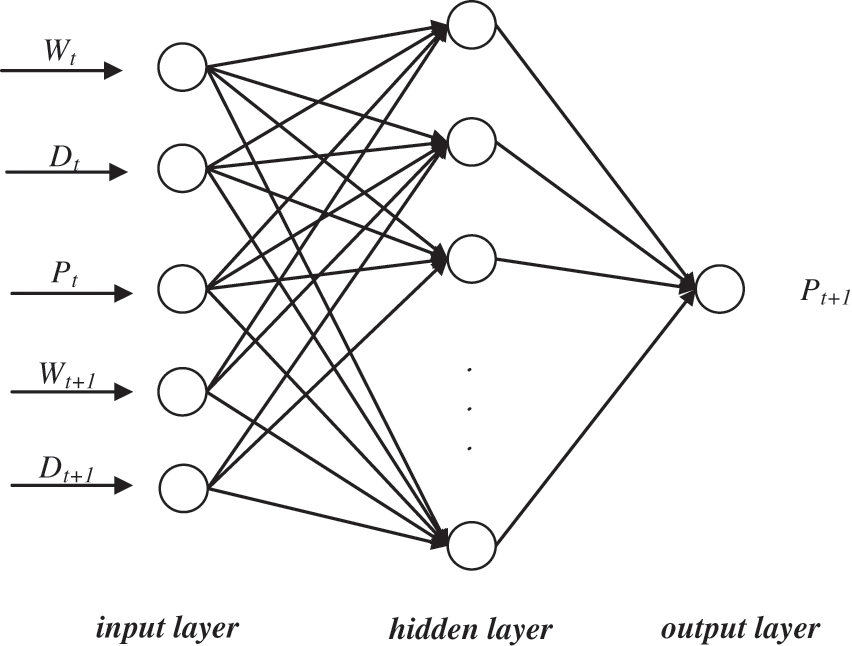
Figure 1: Basis structure of back propagation neural network

BP neural network for wind power prediction, the model parameters tend to fall into local minima and not get the global optimum. Genetic Algorithm (GA), formed by biological evolution and genetics, has the advantages of excellent adaptiveness, parallel processing and no dependence on gradients, but GA tends to fall into local optimum prematurely. Therefore, the GA is improved by adaptively changing the crossover probability value pc and variation probability value pm through the sigmoid function. When the population diversity is poor, increase pc and pm to improve the variation probability of inferior individuals and produce more superior individuals; when the population diversity is high, decrease pc and pm to improve the superior individuals of the population, so that the population can obtain the global optimum value. The BP neural network is optimized using the Improved Adaptive Genetic Algorithm (IAGA), which optimizes the initial weights and thresholds of the BP neural network to find the optimal individuals of the population. The WT-IAGA-BP neural network modeling process is shown in Fig. 2.

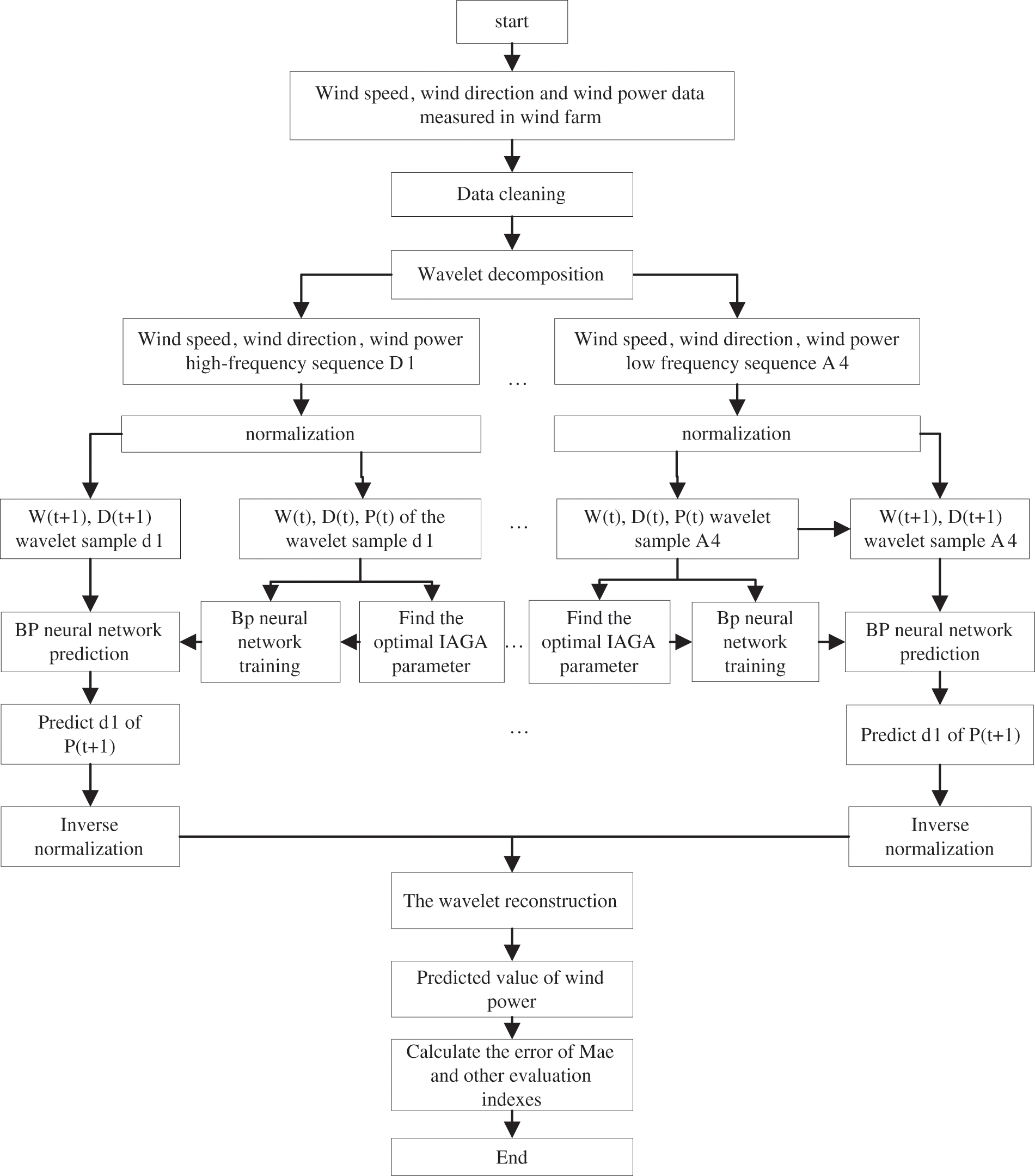
Figure 2: Flowchart of WT-IAGA-BP Wind power prediction model

3.2 Principles of BiLSTM-Based Wind Power Prediction

The Long Short-Term Memory (LSTM) model was devised by Hochreiter et al. To overcome the gradient disappearance of RNN networks, input gates, output gates, and forgetting gates were introduced into the neurons to control the state variables of LSTM neurons. The introduction of logic gates captures the temporal correlation characteristics of data signals, enables a long time effective data storage and acquisition, and avoids the gradient vanishing of RNN networks. The unidirectional LSTM network can process time series data forward, while the Bi-directional Long Short-Term Memory (BiLSTM) network can process time series data forward and backward in parallel. As wind power data is time-series data, the bi-directional nature of the BiLSTM network enables the deep mining of correlation information between time-series wind power data and the search for implied regular relationships between the input data. The BiLSTM network structure is shown in Fig. 3.

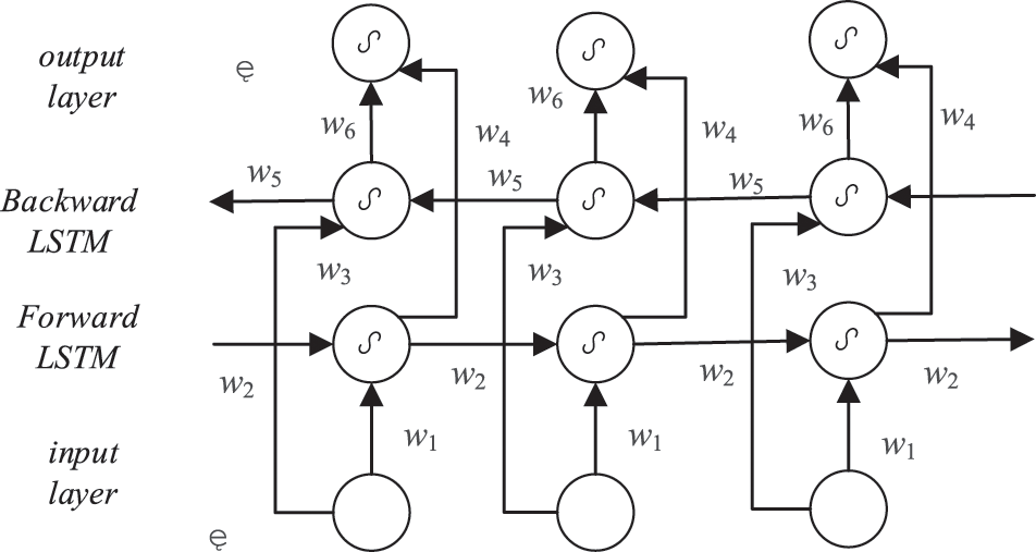
Figure 3: Basic structure of BiLSTM network

The forward layer is connected to the output layer together with the backward layer, sharing the weights w1, w2, w3, w4, w5, and w6. When the network layer is computed forward, the forward layer is computed forward from moment 1 to moment t and the output of the backward hidden layer is stored at each moment. In the reverse direction, the backward layer is computed backward along moment t to moment 1 and the output of the backward implicit layer is stored at each moment. Finally, the outputs of the forward and backward layers are combined to output the final predictions of the model.

The implied layer state ht→ of the forward LSTM network at moment t of the BiLSTM is calculated from the state ht−1→ at moment t−1, as shown in Eq. (10).

ht→=f(w1xt+w2ht−1→)(10)

where ht→ is the implied layer state of the forward LSTM network at moment t; xt is the input at moment t, and ht−1→ is the implied layer state of the forward LSTM network at moment t−1.

The implied layer state ht← of the BiLSTM at moment t of the inverse LSTM network is calculated from the state ht−1← at moment t−1, as shown in Eq. (11).

ht←=f(w3xt+w5ht−1←)(11)

where ht← is the hidden layer state of the inverse LSTM network at time t;ht−1← is the hidden layer state of the inverse LSTM network at time t−1.

The final neuronal output, is shown in Eq. (12).

ot=g(w4xt+w6ht′)(12)

where ht′ is the overall hidden state of the network.

3.3 Principles of Wind Power Prediction Based on the Combination of WT-IAGA-BP and BiLSTM

The main steps of the wind power short-term prediction based on the combination of WT-IAGA-BP and BiLSTM are as follows. The structure of the wind power short-term prediction model based on the combination of WT-IAGA-BP and BiLSTM is shown in Fig. 4.

(1)   The original data is first cleaned to remove abnormal data values and fill in the missing data, thus improving the accuracy of the prediction model. At the same time, the wind power data is normalized to improve the efficiency of the model operations.

(2)   Due to the randomness, volatility, and intermittency of wind power data, compared with the direct use of raw data for wind power prediction, the wavelet decomposition can fully extract the time domain signal and frequency domain signal in a given time series, which has a strong signal characterization capability and improves the model prediction accuracy. Therefore, dbN wavelets are used to carry out wavelet decomposition of wind power data, the number of layers of decomposition is selected, and the decomposed high and low-frequency signals are finally obtained. Among them, the low-frequency signal sequence responds to the wind power variation trend, and the high-frequency signal sequence responds to the high-frequency characteristics of wind speed, humidity, temperature, air pressure, wind direction, and other climatic factors.

(3)   The asymmetric IAGA-BP neural network and BiLSTM network models are selected for the prediction of data at different frequencies. The parameters of the asymmetric IAGA-BP neural network and the BiLSTM network model are adjusted according to the specific decomposition data characteristics, and the BiLSTM network is optimized using Adam. The Dropout strategy is also used in the BiLSTM deep network model. As too many parameters such as the number of hidden layers, the number of neurons in the hidden layer, and the weights of the deep neural network model can easily lead to overfitting, the Dropout strategy is used in the BiLSTM deep network model to randomly select nodes to modify the structure of the neural network itself, to improve the generalization power of the model and avoid overfitting [24–26].

(4)   Based on the simulation results of the prediction model, the optimal parameters of the combined model are found. The prediction values of each series are back-normalized and the series model with high prediction accuracy is selected for the adaptive weight combination according to the prediction accuracy of each time-series data. The prediction results are also reconstructed to obtain the wind power values at the predicted time points.

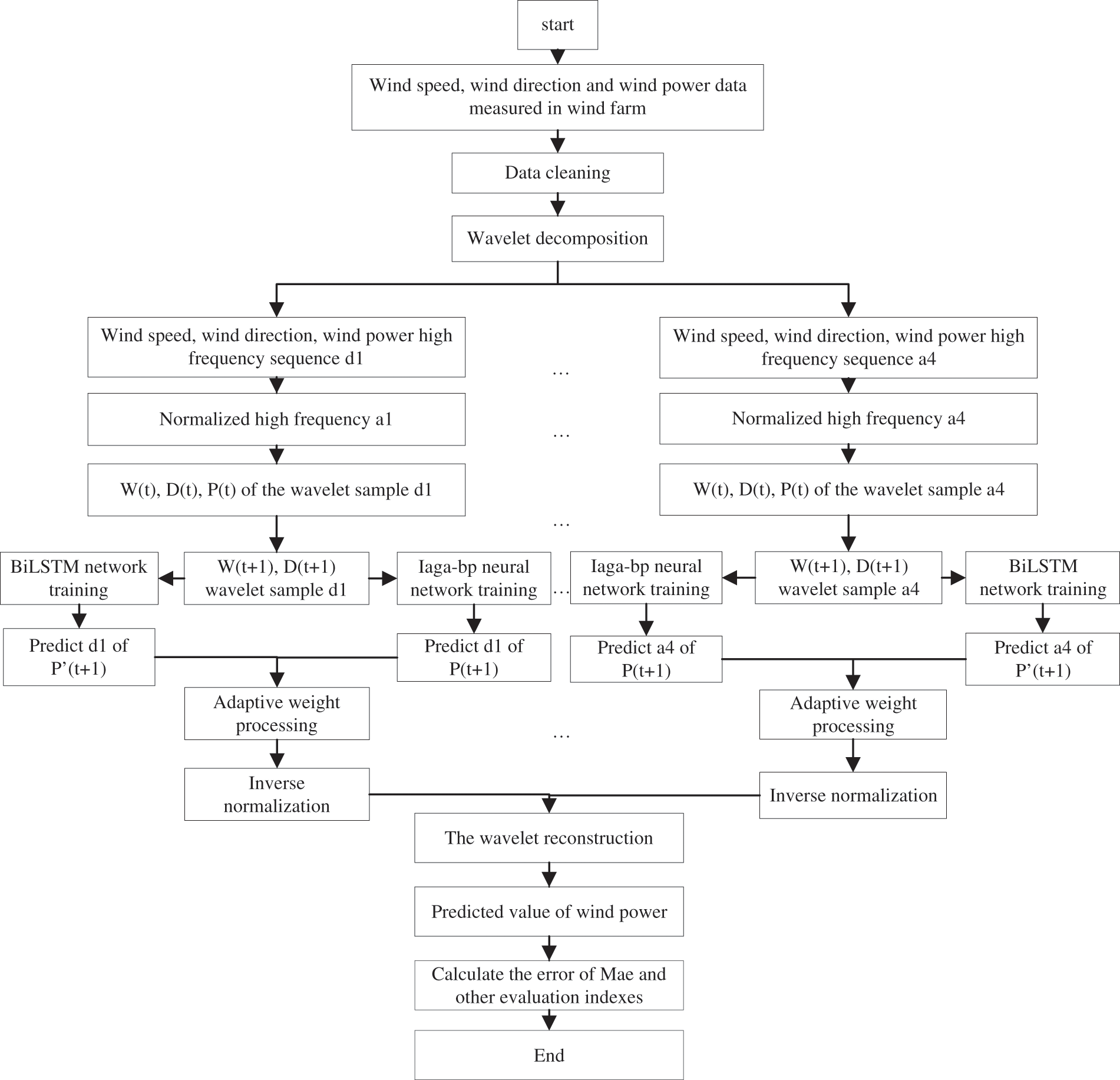
Figure 4: Flowchart of WT-IAGA-BP neural network and BiLSTM network combined model

The output power of wind turbines is mainly affected by the wind speed and wind direction of the wind farm, which requires wind speed and wind direction meteorological information as well as historical wind power as input. Xt=[xtv, xtd, xt, xt−1,…, x2, x1] (t∈[1, n]), xtv, xtd, xt are the wind speed, wind direction, and power at time t. YBP=[y1i,y2i,y3i,…,yni] is the wind power predicted output by WT-IAGA-BP neural network, while YBL=[y1j,y2j,y3j,…,ynj] is the wind power predicted output by the BiLSTM network. To reduce the prediction error of the combined model, the adaptive weighting method is adopted to combine the models. The weighting module obtains the final wind power prediction value Y by assigning different weights adaptively to the wind power forecasted outputs of different prediction models and by linearly summing YBP and YBL, and the final predict value is Y=[y1,y2,y3,…,yn]. The adaptive combination weights are calculated as shown in(13)–(15).

Y1=α1YBP(13)

Y2=a2YBL(14)

Y=Y1+Y2(15)

where α1 and α2 are the weight matrices of different predict models, and the optimal values of α1 and α2 are obtained during the training process of the combined prediction model.

The weight matrix can be computed by formula shown in Eqs. (16) and (17).

E=1n∑t=1n⁡|yt−y^tyt|(16)

ah=|1Eh|∑h=1m⁡|1Eh|(17)

where yt represents the actual wind power at time t and y^t is the predicted wind power at time t. besides, Eh denotes the MAE value of the h-th sequence for forecasting model and ah is the combined weight of the h-th sequence.

4  Simulation Experiments

4.1 Raw Data Processing

This paper takes the Sotavento wind farm in Spain, with a total installed capacity of 17.56 MW, as the research object, and collects some historical data on the wind farm, including wind speed, wind direction, and historical wind power data of the wind farm. The sampling interval of the wind power historical data was 10 min, and the sampling points of the first 12 days of the data (1∼1728) were taken to construct the training samples; the sampling points of the last 3 days of the data (1729∼2160) were used for the prediction samples. As the wind power of the wind farm was predicted, the wind farm power generation collected every 10 min was multiplied by 6 to convert the wind power data.

Daubechies (dbN) series wavelets have better time domain localization analysis and frequency splitting capability and are commonly used for detecting and splitting abnormal signals, etc. The decomposed signal has better smoothness than other wavelet decompositions. The wavelet decomposition is carried out on the original wind speed, wind direction, and power data, and different wavelet functions and decomposition layers are selected for the wavelet decomposition, and the signal reconstruction errors are shown in Table 1.

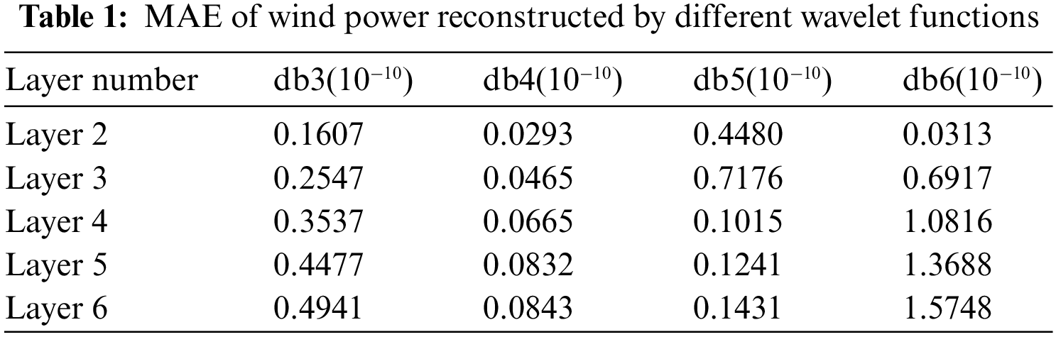
It can be seen from Table 1 that the MAE value will get greater with the increase of layers and different decomposition methods supply different MAE values at different layers. To be specific, though db3, db4, db5, and db6 can smoothly process the decomposition of non-smooth signals, but the reconstruction error of the db4 wavelet is the least among all methods. Therefore, the optimal layer number of decomposition is the layer 4 of the db4 wavelet. In short, layer 4 of the db4 wavelet is chosen to decompose the wind power data to effectively extract the implied feature signals of wind power data at each frequency and reduce the influence of wavelet reconstruction error on the prediction accuracy.

4.2 Model Evaluation Metrics

Wind power forecasts deviate from the actual values, and the magnitude of the error provides a basis for judging the merits of the forecasting model. To study the effect of wind power prediction, Mean Absolute Error (MAE), Root Mean Square Error (RMSE), coefficient of determination (R2), and Maximum Absolute Error (MAE) are used as evaluation indicators. MAE represents the mean of absolute error between predicted and actual values, as shown in Eq. (18). RMSE is the standard deviation of the residuals between the predicted and true values. When the curve fits the data, the smaller the RMSE value, the better the performance of the prediction model, as shown in Eq. (19). R2 indicates the degree of correlation between the two variables. The closer the R2 is to 1, the better the fitted regression effect and the stronger the correlation, as shown in Eq. (20).

MAE=∑i=1n⁡|XSi−XYi|n(18)

RMSE=∑i=1n⁡(XSi−XYi)2n(19)

R2=∑i=1n⁡(XYi−XYp)2∑i=1n⁡(XSi−XSp)2(20)

where XSi, XYi are the measured and predicted wind power at the ith sampling point, respectively.XSP,XYP are the mean measured and predicted power, respectively; n is the number of predicted samples.

Due to the different datasets used in the forecasting models in the literature, it is not easy to compare the forecasting effects of different models. To facilitate a comparison of the effects of the combined forecasting models proposed in this paper, the Normalised Mean Absolute Error (NMAE), as shown in Eq. (21), and the Normalised Root Mean Square Error (NRMSE) were used to evaluate the forecasting effects, as shown in Eq. (22).

NMAE=∑i=1n⁡|XSi−XYi|n×100P%(21)

NRMSE=∑i=1n⁡(XSi−XYi)2n×100P%(22)

where P is the installed capacity of the wind farm.

4.3 Analysis of Experimental Results

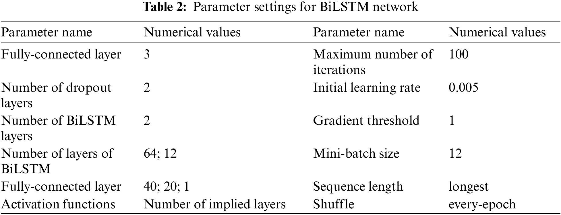
To verify the effectiveness of wind power short-term prediction by combining WT-IAGA-BP with BiLSTM, single model LSTM, BiLSTM, WT-LSTM, WT-BiLSTM, WT-IAGA-BP, and combined WT-IAGA-BP and LSTM models were used for comparison. In this paper, the BiLSTM parameters are set as shown in Table 2 through extensive experiments and the characteristics of each frequency signal.

The db4 wavelet was used to decompose the historical data Wt, Dt, Pt, and the predicted moment data Wt+1 and Dt+1 in 4 layers, and the subseries of the 4-layer (a4, d1, d2, d3, d4) decomposition were used in turn to construct the WT-LSTM, WT-BiLSTM, WT-IAGA-BP, WT-IAGA-BP, and LSTM combined prediction models, WT-IAGA-BP and BiLSTM combined prediction models so that they predict the wind power of the subseries after the 4-layer decomposition of the db4 wavelet, and then the wind power of each of the 4-layer (a4, d1, d2, d3, d4) subseries predicted by WT-LSTM, WT-BiLSTM, and WT-IAGA-BP are superimposed separately. WT-IAGA-BP and LSTM combined model, WT-IAGA-BP with BiLSTM combined model requires the combination of the predicted subsequences by adaptive weights and the superposition of the combined sequences. Meanwhile, the LSTM and BiLSTM models were used for comparison to obtaining seven wind power prediction results, as shown in Fig. 5.

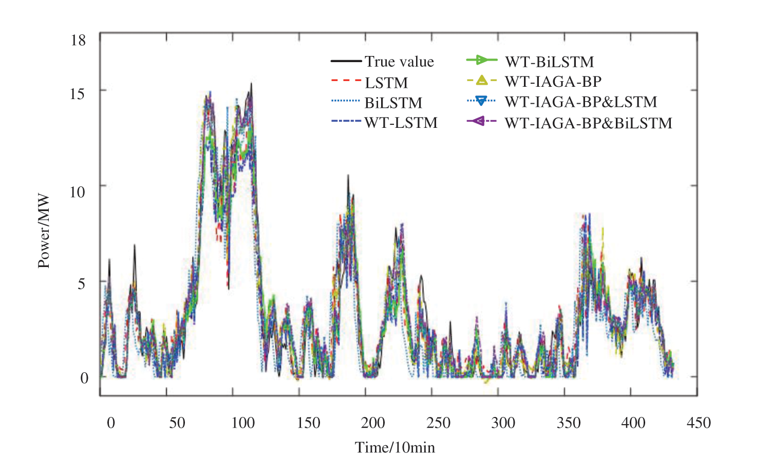
Figure 5: Comparison of wind power prediction results with different models

In the whole process of wind power prediction, compared with the single models LSTM, BiLSTM, WT-LSTM, WT-BiLSTM, WT-IAGA-BP, and the combined model of WT-IAGA-BP and LSTM, the wind power short-term prediction model based on the combination of WT-IAGA-BP and BiLSTM can track the wind power in time, and the predicted wind power values are closer to the actual values and the prediction system is more stable. To minimize the overall error, the combined neural network-based prediction model tends to be more stable than the single prediction model. In the case of sudden changes in wind power, combining the results of each series predicted by the WT-IAGA-BP model and BiLSTM model with adaptive weights, as well as reconstructing the combined subsequence, will effectively reduce the fluctuation of wind power prediction values. The wind power prediction curves of the combined models are smoother than those of the single models, and there is no abrupt change in the prediction errors at the prediction time points. The combined prediction models are important for improving the wind power consumption capacity and ensuring the safe operation of the grid. The statistical values of the error indicators for each prediction model are shown in Table 3.

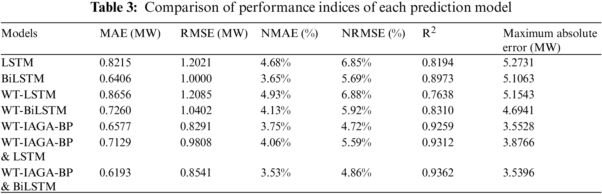
After data cleaning, to evaluate the short-term prediction effect of the combined WT-IAGA-BP and BiLSTM model, the prediction evaluation indexes of db4 decomposed into 4 layers were calculated. From Table 2, it can be seen that the MAE and RMSE of WT-LSTM increased by 4.41% and 0.64%, respectively. Compared with LSTM, NMAE and NRMSE of WT-LSTM increased by 0.25% and 0.03%, respectively, and R2 decreased by 5.56%. Compared with BiLSTM, the MAE and RMSE of WT-BiLSTM increased by 8.54% and 4.02%, NMAE and NRMSE increased by 0.49%, 0.23%, R2 decreased by 6.63%, and the maximum absolute error decreased by 0.4122 MW. Comparing the prediction results, wavelet decomposition prediction can reduce the maximum error of prediction and improve the stability of the prediction model. At the same time, Adam’s algorithm can effectively optimize the BiLSTM network, so that BiLSTM can fully learn the correlation information between wind power data. The Dropout strategy can avoid overfitting the BiLSTM prediction model during the training of the BiLSTM prediction model.

When compared to WT-LSTM, the MAE and RMSE of the combined model of WT-IAGA-BP and BiLSTM decreased by 24.64% and 35.44%, NMAE and NRMSE decreased by 1.40% and 2.02% respectively, R2 increased by 17.24% and the maximum absolute error decreased by 1.6147 MW. When it comes to theWT-BiLSTM, the MAE and RMSE of the combined model of WT-IAGA-BP and BiLSTM decreased by 10.67% and 18.61%, NMAE and NRMSE decreased by 0.60% and 1.06% respectively, R2 improved by 10.52%, and the maximum absolute error decreased by 1.1545 MW. The MAE and NMAE of the combined model of WT-IAGA-BP and BiLSTM decreased by 3.84% and 2.02% respectively compared with WT-IAGA-BP, respectively. While RMSE, NRMSE, and R2 improved by 2.50%, 0.14%, and 1.03%, respectively, and the maximum absolute error decreased by 0.0132 MW. While MAE, RMSE and R2 of the combined model of WT-IAGA-BP and BiLSTM is better than that of WT-IAGA-BP& LSTM 9.36% and 12.67%, and R2 increased 0.5%, respectively. The results show that the combined prediction model based on WT-IAGA-BP and BiLSTM can overcome the limitations of a single model and improve the stability and accuracy of the prediction model during sudden changes in wind power.

The above simulation results and analysis show that the establishment of a short-term wind power prediction model based on the combination of WT-IAGA-BP and BiLSTM has a stable global optimization finding capability, which can effectively reduce the volatility of the prediction system and provide accurate wind power prediction. Compared with LSTM, BiLSTM, WT-LSTM, WT-BiLSTM, WT-IAGA-BP, and the combined WT-IAGA-BP and LSTM model, the prediction stability and accuracy of the combined WT-IAGA-BP and BiLSTM prediction model are substantially improved, and its prediction results are optimal. When the wind power changes, the prediction results of each series of the WT-IAGA-BP model and BiLSTM model are combined by adaptive weights, and the combined subsequence is reconstructed, which can effectively reduce the fluctuation of the wind power prediction value of the single model. The wind power short-term prediction model based on the combination of WT-IAGA-BP and BiLSTM can better track wind power, minimize the scale of deviation of the predicted value from the true value and maintain high prediction accuracy. It provides a new solution for the short-term prediction of wind power, and at the same time provides a theoretical basis for power generation planning, peak and frequency regulation, and tide optimization.

5  Conclusion

To improve the prediction accuracy, this paper proposes a combination of WT-IAGA-BP and BiLSTM for the short-term prediction of wind power. Firstly, IAGA is introduced to optimize the BP neural network weights and thresholds to avoid the BP neural network weights and thresholds falling into local optimum. Secondly, the db4 wavelet is used to decompose the wind power data in 4 layers to filter the noise signals in the data. Then, the BiLSTM network was used to fuse the multimodal data using the bi-directional nature of the BiLSTM, and the BiLSTM was optimized using Adam. At the same time, the Dropout strategy was applied to avoid overfitting of the BiLSTM, and the adaptive weights were used to combine the single model prediction results. Finally, simulation analysis is performed and compared with LSTM, BiLSTM, WT-LSTM, WT-BiLSTM, WT-IAGA-BP, WT-IAGA-BP & LSTM prediction models. The experimental results show that the combined wind power short-term prediction model based on WT-IAGA-BP and BiLSTM avoids the over-learning of deep learning in the case of poor data quality, and can overcome the prediction errors caused by the non-linearity, uncertainty, and randomness of traditional prediction models. The model proposed in this paper has stronger robustness and adaptability, and its prediction accuracy is higher, which can provide a theoretical basis for improving the level of wind power consumption and ensuring stable grid operation. However, the WT-IAGA-BP neural network and BiLSTM network prediction models are built separately using sequence data of different frequencies after wavelet decomposition, which increases the complexity and computational power of the combined model structure and reduces the training efficiency of the model.

Funding Statement: The authors gratefully acknowledge financial support of national natural science foundation of China (No. 52067021), natural science foundation of Xinjiang (2022D01C35), excellent youth scientific and technological talents plan of Xinjiang (No. 2019Q012) and major science & technology special project of Xinjiang Uygur Autonomous Region (2022A01002-2)

Conflicts of Interest: The authors declare that they have no conflicts of interest to report regarding the present study.

References

1. Y. R. Wang, Y. Yu and S. Y. Cao, “A review of applications of artificial intelligent algorithms in wind farms,” Artificial Intelligence Review, vol. 53, no. 5, pp. 3447–3500, 2020. [Google Scholar]

2. D. Xu, H. Shao, H. X. Deng and X. Wang, “The hidden-layers topology analysis of deep learning models in survey for forecasting and generation of the wind power and photovoltaic energy,” Computer Modeling in Engineering & Sciences, vol. 131, no. 2, pp. 567–597, 2022. [Google Scholar]

3. D. Z. Li and Y. Y. Li, “Ultra-short-term wind power prediction based on deep learning with error correction,” Journal of Solar Energy, vol. 42, no. 12, pp. 200–205. 2021. [Google Scholar]

4. Z. Tarek, M. Y. Shams and A. M. Elshewey, “Wind power prediction based on machine learning and deep learning models,” Computers, Materials & Continua, vol. 74, no. 1, pp. 715–732, 2023. [Google Scholar]

5. X. Deng and H. Shao, “Deep learning approach with optimized hidden-layers topology for short-term wind power forecasting,” Energy Engineering, vol. 117, no. 5, pp. 279–287, 2021. [Google Scholar]

6. R. Yu, Z. Liu, J. Wang, M. Zhao and J. Gao, “Analysis and application of the spatio-temporal feature in wind power prediction,” Computer Systems Science and Engineering, vol. 33, no. 4, pp. 267–274, 2018. [Google Scholar]

7. Y. Zhang, H. X. Sun and Y. J. Guo, “Wind power prediction based on PSO-SVR and grey combination model,” IEEE Access, vol. 7, pp. 136254–136267, 2019. [Google Scholar]

8. C. S. Li, G. Tang and X. M. Xue, “Short-term wind speed interval prediction based on ensemble GRU model,” IEEE Transactions on Sustainable Energy, vol. 11, no. 3, pp. 1370–1380, 2020. [Google Scholar]

9. Q. M. Feng and S. P. Qian, “Research on the prediction of short-term wind power based on wavelet neural networks,” Energy Reports, vol. 8, pp. 553–559, 2022. [Google Scholar]

10. J. Q. An, F. Yin and M. Wu, “Multisource wind speed fusion method for short-term wind power prediction,” IEEE Transactions on Industrial Informatics, vol. 17, no. 9, pp. 5927–5937, 2020. [Google Scholar]

11. X. Deng, H. Shao, C. Hu, D. Jiang and Y. Jiang, “Wind power forecasting methods based on deep learning: A survey,” CMES-Computer Modeling in Engineering & Sciences, vol. 122, no. 1, pp. 273–301, 2020. [Google Scholar]

12. Y. S. Wang, J. Gao and Z. W. Xu, “A prediction model for Ultra-short-term output power of wind farms based on deep learning, ” International Journal of Computers Communications & Control, vol. 15, no. 4, pp. 3901, 2020. [Google Scholar]

13. L. Yan and W. Hong, “Evaluation and forecasting of wind energy investment risk along the belt and road based on a novel hybrid intelligent model,” Computer Modeling in Engineering & Sciences, vol. 128, no. 3, pp. 1069–1102, 2021. [Google Scholar]

14. Y. R. Wang, D. C. Wang and Y. Tang, “Clustered hybrid wind power prediction model based on ARMA, PSO-SVM, and clustering methods,” IEEE Access, vol. 8, pp. 17071–17079, 2020. [Google Scholar]

15. M. Zhang, H. Li and X. Deng, “Inferential statistics and machine learning models for short-term wind power forecasting,” Energy Engineering, vol. 119, no. 1, pp. 237–252, 2022. [Google Scholar]

16. A. Kisvari, Z. Lin and X. L. Liu, “Wind power forecasting-A data-driven method along with gated recurrent neural network,” Renewable Energy, vol. 163, pp. 1895–1909, 2021. [Google Scholar]

17. Y. H. Sun, P. Wang and S. W. Zhai, “Ultra short-term probability prediction of wind power based on LSTM network and condition normal distribution,” Wind Energy, vol. 23, no. 1, pp. 63–76, 2019. [Google Scholar]

18. L. Huang, L. X. Li and X. Y. Wei, “Short-term prediction of wind power based on BiLSTM-CNN-WGAN-GP,” Soft Computing, vol. 26, no. 20, pp. 10607–10621, 2022. [Google Scholar]

19. J. X. Wang, B. Deng and J. Wang, “Short-term wind power prediction based on empirical modal decomposition and RBF neural network,” Journal of Power Systems and Automation, vol. 32, no. 11, pp. 109–115, 2020. [Google Scholar]

20. Z. X. Xing, B. Y. Qu and Y. Liu, “Comparative study of reformed neural network based short-term wind power forecasting models,” IET Renewable Power Generation, vol. 16, no. 5, pp. 885–899, 2022. [Google Scholar]

21. X. B. Ma, “Short-term wind power prediction based on wavelet transform and BP neural network,” Journal of Power Science and Technology, vol. 30, no. 2, pp. 92–97, 2015. [Google Scholar]

22. R. H. Cui, W. D. Hu and L. K. Geng, “Wavelet-based reconstruction of signal singularities for aerial fault arc detection,” Electrical Drives, vol. 48, no. 6, pp. 69–72, 2018. [Google Scholar]

23. X. Y. Pu, G. H. Bi and K. Wang, “Ultra-short term forecast of wind power based on FEEMD-PACF_AdaBoost model,” Computer Application and Software, vol. 38, no. 11, pp. 91–97, 2021. [Google Scholar]

24. X. Liu, Y. P. Han and Z. P. Liu, “Research on groundwater depth prediction method based on BiLSTM-NFC,” Yellow River, vol. 43, no. 6, pp. 80–85, 2021. [Google Scholar]

25. H. Zhang, C. H. Hu and D. B. Du, “Remaining useful life prediction method of Lithium-Ion battery based on Bi-LSTM network under Multi-State influence,” ACTA Electronica Sinica, vol. 50, no. 3, pp. 619–624, 2022. [Google Scholar]

26. Y. Huang, C. H. Chen and C. J. Huang, “Motor fault detection and feature extraction using RNN-based variational auto-encoder,” IEEE Access, vol. 7, pp. 139086–139096, 2019. [Google Scholar]