Atrous Convolution-Based Residual Deep CNN for Image Dehazing with Spider Monkey–Particle Swarm Optimization

1  Introduction

Haze is regarded as a phenomenon due to the atmosphere, in which the dry particles, dust, or aerosols reduce the image scene quality. Haze generally makes specific degradation in the scene quality of the image, capping the total color contrastand making occlusion of objects present in the scene due to ambient light [1]. The haze effect [2] causes low visual quality and diminished color contrast in real-world images taken in cloudy weather conditions. Various computer vision tasks like autonomous driving system and Land Use Land Cover (LULC) detection is performed by monitoring the real-world images and scene evaluation with satellite images that rely on the clean images to obtain accurate results. Therefore it is essential to reduce the haze effect over the captured images to enhance the images visual quality and the process of object recognition and detection [3]. The image haze formation model [4] is shown in Fig. 1.

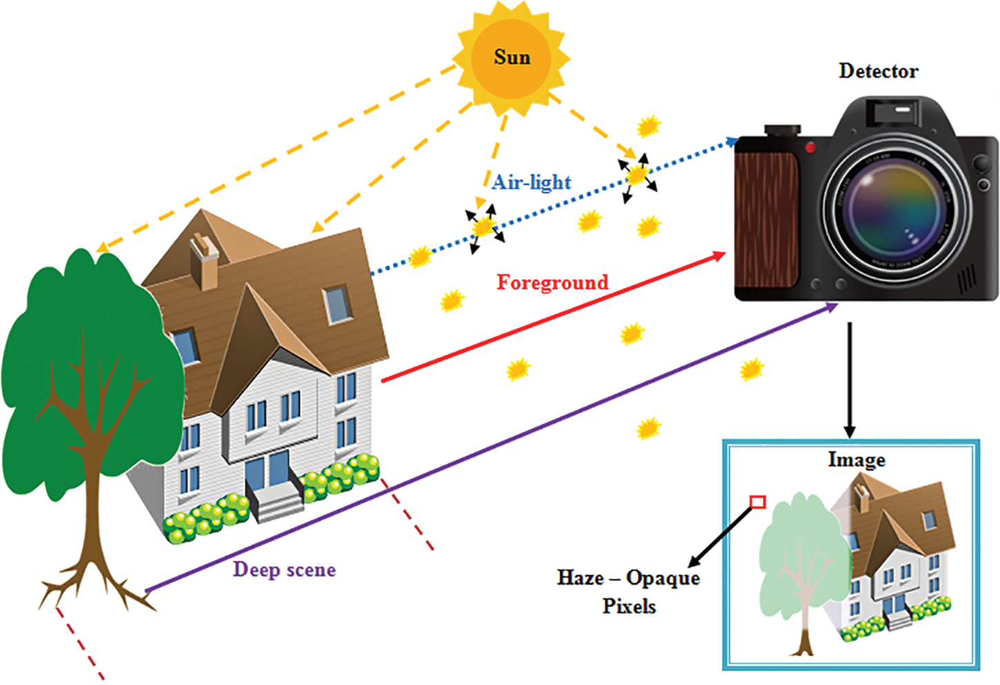
Figure 1: Image haze formation

According to the theory of haze model [5,6], the influence of atmospheric light on natural images can be described as in Eqs. (1) and (2) by

I(m,n)=J(m,n)⋅T(m,n)+A(1−T(m,n))(1)

T(m,n)=e−βd(m,n)(2)

Here, I and J are hazy and haze-free images, T is the transmission map connected with β (atmospheric scattering coefficient), and d (depth between the camera and scene), A is the global ambient light (atmospheric light) at pixel location (m,n). The haze-free image J is was obtained by transforming Eq. (1) into the following Eq. (3).

J(m,n)=I(m,n)T(m,n)−A(1−1T(m,n))(3)

I(m,n)=J(m,n), when d(m,n)→0, T(m,n)→1(4)

According to Eq. (4) the captured image will be the actual radiance from the scene. But, in the case of terrestrial imaging, the scene depth is very high, and the influence of atmospheric light will be more as described by Eq. (5).

I(m,n)=A, when d(m,n)→∞,T(m,n)→0(5)

Both the cases of Eqs. (4) and (5) are not possible in practical situations. The estimation of T(m,n) and A are essential in obtaining the dehazed image. Accurate estimation of A obtains the detailed dehazed image without losing the microscopic details from the high-intensity regions of the hazy input image.

Many existing model-based dehazing methods [7–9] propose the complex prior regularizations for the approximation of A and T(m,n) for extracting the spatial features from the hazy input, but the approximate image will still be different from the haze-free image. These methods are time-consuming, involve huge parameters, and need help in the optimization.

To overcome the dependence on approximated prior, the design of learning-driven methods using deep learning techniques is promoted. The deep Convolutional Neural Network (CNN) model [10] maps the atmospheric scattering parameters learned from the network training to recover the image from haze effects. Furthermore, wavelet techniques are also used in image dehazing models, where Discrete Wavelet Transform (DWT) [11] divides the images into patches using various wavelet sub-bands or frequencies. To retain the high-frequency information and prevent the pseudo-shadow phenomenon in the dehazed image, the SSIM loss of each image patch is calculated, and the weights are updated.

The image dehazing aims to minimize the haze effect and enhance the contrast levels by maintaining the very fine details at the edges, in this work a new deep learning method for image dehazing using a hybrid swarm optimization algorithm is proposed. The structure of this article is as follows. In Section 2, the existing works related to the image dehazing are introduced. The architectural flow of the proposed image dehazing framework is described along with the appropriate datasets in Section 3. Section 4 defines the wavelet image decomposition and hybrid Spider Monkey Particle Swarm Optimization (SMPSO) algorithm. Section 5 discusses the image dehazing model using Atrous Convolution-based Residual Deep CNN. Section 6 provides the experimental settings, results, and ablation analysis. Section 7 outlines the conclusion and future scope of this work.

2  Related Works

The image dehazing problem is considered as the “No-Reference (NR) Image Quality Assessment (IQA)” method. A superior way of performing image dehazing is to design specific quantitative evaluation metrics. However, this is challenging due to the complications in the image dehazing process as various dehazing algorithms (DHAs) have unique haze effects.

Most image restoration methods from haze rely on the air-light scattering model [12] due to the performance attained in processing the hazy daytime images. These methods are classified into prior-based computation models [5,13] and learning-based prediction models [14–16].

Based on the number of images used for dehazing process, the dehazing methods are classified into multiple images and single image–based haze removal methods. Polarization-based methods [17] use varying degrees of polarization of different images to restore the scene depth. Contrast enhancement methods [18,19], and Multiscale fusion [20] algorithms require a single image which depends on the distinctive traits of the ground truth image.

The application of deep CNN has been increased in the recent research works of image dehazing and achieved a remarkable throughput. These methods result in better recovery of explicit scenes in the image from the haze effects by heuristically learning the complex relations from the haze data observations.

Li et al. [21] proposed calculating the ratio of the foggy image to transmission map estimate with residual-based deep CNN and avoiding estimating atmospheric light. Li et al. [22] present an accurate estimation of atmospheric light and strive to remove the bright region’s effect on estimation using quad-tree decomposition. Liu et al. [23] developed an agnostic CNN model to fully eliminate the necessity for parameter estimation and require no insight into the atmospheric scattering model using local and global residual learning stages. Ren et al. [24] method learn the relation amid the hazy input and the corresponding scene depth using a multiscale deep neural network.

Gan et al. [25] propose to jointly estimate the air-light and transmission maps through a Conditional Generative Adversarial Network (CGAN). Zhang et al. [26] recover the clear scene through high-level features and the scene details from low-level feature maps using Deep Residual Convolutional Dehazing Network (DRCDN). Wang et al. [27] designed an enhanced network based on a CNN-based dehazing model with three different modules within the network. They jointly estimated the air-light and feature map to enhance the ability of CNN. Dharejo et al. [28] proposed using CNN with a wavelet hybrid network in the wavelet domain. The local features and global features are achieved from the multi-level resolution of hazy images.

Yang et al. [29] developed a new deep-learning method combining haze-related prior information and deep-learning architectures perspectives. Wang et al. [30] developed a module for feature extraction using the deep residual haze network and recovers the clear image by subtracting the trained residual transmission map and the corresponding hazy input. Min et al. [31] proposed a DHA quality evaluation method with the integration of haze-relevant features. The technique works better for aerial image databases with image structure recovering and enhancing the low-contrast areas. Yu et al. [32] use the concept of multi-resolution segmentation with an image fusion process for transmission map estimation. Bilal et al. [33,34] reduces the degradation effects in the images using evolutionary optimization algorithm and weighted filter with dilated convolution and watershed segmentation.

3  Proposed Methodology

3.1 Architectural Flow of the Proposed Framework

The combined effect of haze and reflected light from the scene object reduces the contrast, makes the objects in the scene challenging to identify, and creates difficulty in further processing. The learning-based methods utilize machine learning frameworks for apparentimage recovery. The deep neural network is designed to learn the scene depth and haze-based features for the ground truth image.

This article proposes a novel atrous convolution-based residual deep CNN using a hybrid SMPSO algorithm to recover the clear image from hazy input. The proposed framework consists of three major blocks viz., (1) forward wavelet transform, (2) residual deep CNN with atrous convolution using an optimization algorithm, and (3) inverse wavelet transform for reconstructing the dehazed image.

The dataset images are collected and given to the wavelet transform block. It decomposes the input images into four separate frequency-classified sub-bands. The low-frequency sub-image patch contains very fine details and most of the details of the input image, and this image patch will be the input to the deep CNN block.

The proposed network consists of fewer convolution layers, namely, convolution layers (vanilla convolution) and atrous convolution layers (dilated convolution), at the offset of not compromising the performance with the other learning models. This type of filter used in network learning eliminates the possibility of blur in the obtained residual image. The hybrid optimization algorithm optimizes the batch size, epochs, and learning rate during the network training. The residual image was further combined with high-frequency decomposed patches using IDWT to obtain the haze-free output.

Fig. 2 shows the architectural flow of the proposed atrous convolution-based residual deep CNN framework using a hybrid SMPSO algorithm.

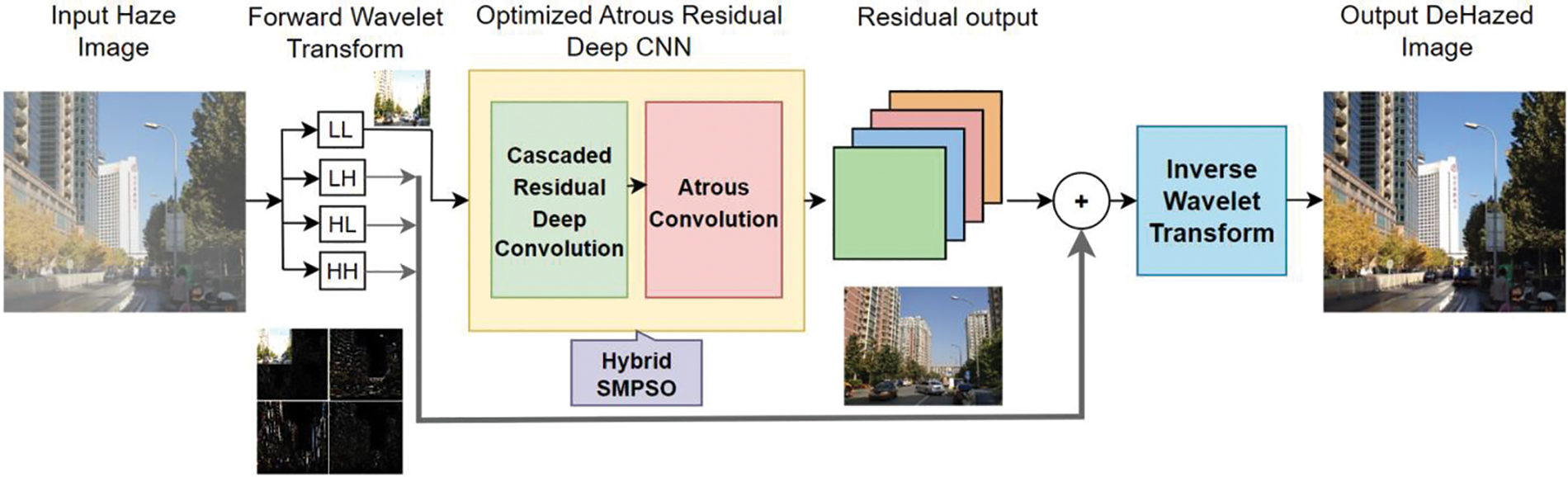
Figure 2: Architectural flow of the proposed image dehazing framework

3.2 Image Dehazing Dataset Collection

The above image dehazing framework is implemented on two different datasets: Synthetic Objective Testing Set (SOTS) [RESIDE], and I-Haze of NTIRE 2018. The details of the datasets are provided below.

SOTS [RESIDE]: The Synthetic Objective Testing Set (SOTS) RESIDE dataset consists of 500 hazy training images under indoor and outdoor subsets, and 50 indoor and 492 outdoor ground truth images. The dataset is accessed from the link “https://www.kaggle.com/datasets/balraj98/synthetic-objective-testing-set-sots-reside”, access date: 2022–05–24.

I-Haze Dataset: The I-Haze dataset is deployed in NTIRE 2018 CVPR dehazing challenge with 30 hazy and ground truth images respectively. The dataset is accessed from the link “https://data.vision.ee.ethz.ch/cvl/ntire18//i-haze/”, access date: 2022–06–19.

4  Wavelet-Based Image Decomposition and Hybrid Swarm Optimization

4.1 DWT-Based Image Decomposition

In the proposed method, before dehazing, DHWT is used to decompose the original hazy input image [35]. As a result, the four distinct sub-bands: approximation (LL), horizontal (LH), vertical (HL), and diagonal (HH) corresponding to the respective wavelet sub-band coefficient extract the information from the hazy input. The LL sub-band corresponds to the hazy input’s down-sampled version (↓2). The LH and HL sub-bands tend to isolate the horizontal and vertical features, and the HH sub-band preserves the corresponding localized high-frequency point features in hazy input. The low-frequency sub-image is considered for dehazing using atrous convolution-based residual deep CNN, and the high-frequency sub-images retain the high-frequency hazy input details. In the end, the clear image was recovered by applying the IDWT for the combined residual image and the high-frequency component of the wavelet transform.

Corresponding to four wavelet sub-bands seen above, one scaling function ϕLL(cc,dd) and three wavelet functions (ψLH(cc,dd), ψHL(cc,dd) and ψHH(cc,dd)) are shown in Eq. (6).

ϕLL(cc,dd)=ϕL(cc)ϕL(dd)ψLH(cc,dd)=ψL(cc)ψH(dd)ψHL(cc,dd)=ψH(cc) ψL(dd)ψHH(cc,dd)=ψH(cc) ψH(dd)}(6)

The IDWT coefficients can be obtained through the Haar wavelet by using the Eq. (7).

A=A1+B1+C1+D1B=A1−B1+C1−D1C=A1+B1−C1−D1D=A1−B1−C1−D1}(7)

here, A, B, C, and D are the input image pixel values and A1, B1, C1, and D1 are the corresponding one-level wavelet decomposed image pixel values as shown in Fig. 3.

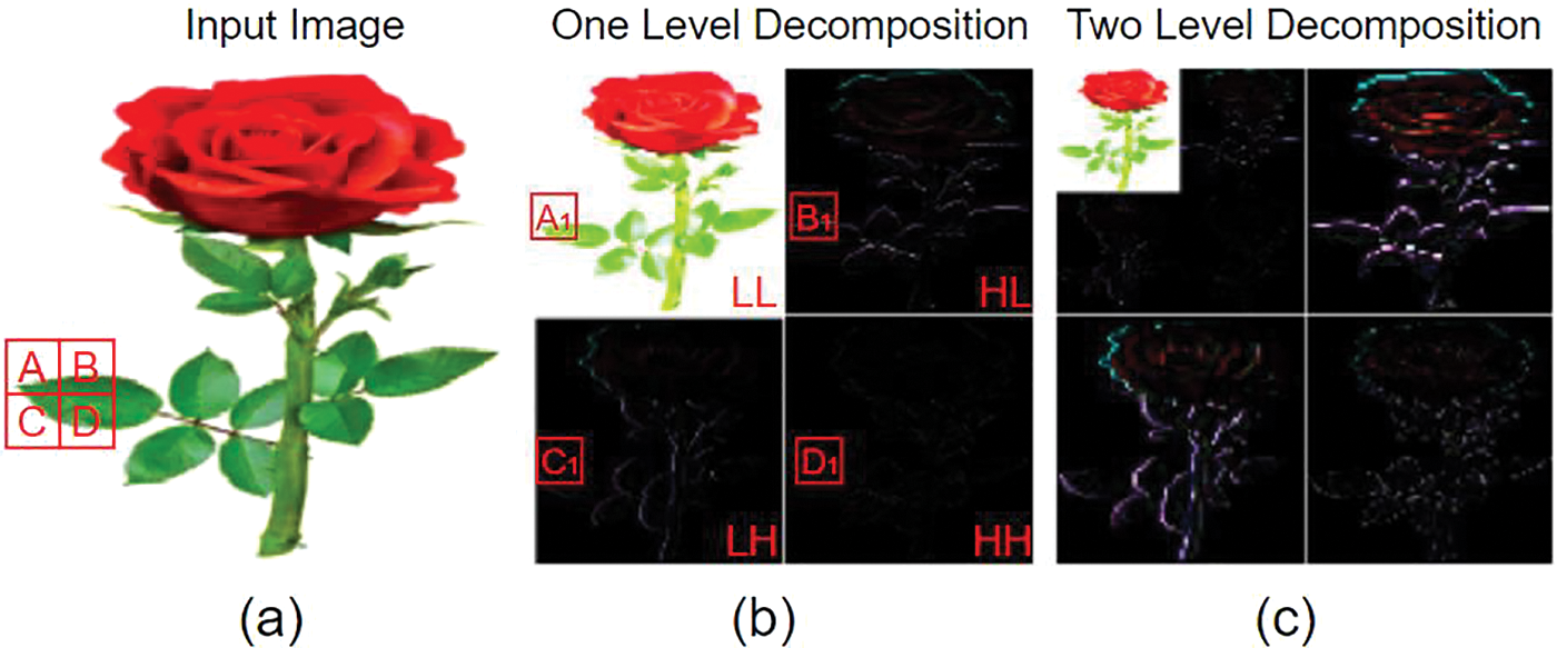
Figure 3: (a) Input image, (b) one-level decomposition of the input image, (c) two-level decomposition of the same

4.2 Meta-Heuristic Swarm-Based Hybrid SMPSO Algorithm

A single optimization algorithm cannot address the full aspects of all search and optimization issues. Because each optimization will have distinct merits and demerits, combining the features of these optimizations enable to development of a hybrid algorithm for better robustness and more flexibility to solve complicated issues [36]. The hybrid SMPSO algorithm combines the PSO and SMO algorithms, is presented in this section.

4.2.1 Particle Swarm Optimization (PSO) Algorithm

The swarm intelligence-based algorithms have gained wide popularity and are addressed in many engineering optimization issues. PSO is an adaptable and particle-based heuristic search optimization for solving engineering optimization problems proposed by Eberhart, R. Kennedy, J and Shi [37,38].

According to PSO, any problem is computationally expensive and can be solved by finding the best solution that fits into it using an exploration and exploitation strategy. The algorithm is broadly accepted due to its superior and fast convergence to optimum, high accuracy, and low memory requirements. The optimization randomly initializes a set of particles (candidate solutions) called a swarm flying in the search space of z-dimension. The vector form of velocity Vi is Vi = (vi1,….viz) and position Xi is Xi = (xi1,….xiz) of each particle i and will update based on the particle’s individual experience and that of its neighbors as in Eqs. (8.a) and (8.b).

Vik+1=ωVik+c1r1(Pbik− Xik)+c2r2(Gbik− Xik)(8.a)

Xik+1=Xik+Vik+1(8.b)

where i = 0, 1,…N−1,Vik and Xik is the current velocity and position of the particle i at kth iteration, Vik + 1 is updated velocity of particle i at (k+1)th iteration with inertia weight ω, acceleration coefficients (c1 and c2), and r1, r2 are evenly distributed arbitrary numbers between (0, 1) generated for each iteration. The best possible position for particle i is Pbik and the best possible position among the population until kth iteration is Gbik.

Every particle i will update using yi, the best solution for particle i in the local search space, and y*(k), the position that yields the best solution among all the yi’s in the global search space. The Pbi and Gbi values will be updated at iteration k with a swarm of N particles using Eqs. (9) and (10).

yi(k+1)={xi(k+1),if f(yi(k))>f(Pbi)yi(k),if f(yi(k))≤f(Pbi)(9)

y∗(k)∈{y1(k), y2(k), … yN(k)},

f(y∗(k))=min{f(y1(k)), f(y2(k)), …f(yN(k))}(10)

The acceleration coefficients control the particle speed at each iteration. In Eq. (11) the time-varying inertia weight ω controls the PSO algorithm’s convergence and linearly decreases over time. The high value of inertia weight during the early stages of search facilitates the chance of global exploration (visiting more positions in the search range) and low value in the later stages facilitates local exploration (for local search ability).

inertia weight ω=(ω1−ω2)(max.allowable iter. iter.currentiter.current)+ω2(11)

where ω1 and ω2 represent the inertia weight’s initial and final values respectively.

4.2.2 Spider Monkey Optimization (SMO) Algorithm

It is a swarm intelligence-based optimization influenced by the spider monkeys’ Fission-Fusion Social (FFS) behavior during the foraging process. The characteristics of the SMO algorithm [39] depend on the grouping of monkeys into groups from small to large and vice-versa. The SMO contains four phases: Local Leader Phase (LLP), Global Leader Phase (GLP), Learning Phase, and Decision phase.

Let Xi represents the ith individual in a k-dimension vector of the swarm population, each ith individual is initialized as in Eq. (12):

Xik=Xmink+U(0,1)×(Xmaxk−Xmink)(12)

where Xminkj and Xmaxk are the boundary values of the search space. U(0, 1) is an evenly distributed arbitrary number between (0, 1).

During LLP, the individuals adapt their positions using the group member’s and local leader knowledge in their group. The updation in new position is based on the individual’s fitness and the perturbation rate probability. The new position update Eq. (13) is:

Xik+1=Xik+U(0,1)×(LLmk−Xik)+U(−1,1)×(Xrk−Xik)(13)

where Xik+1 is the ith individual in kth dimension, LLmk represents the local leader, and Xrk is the arbitrary selected individual from the mth group so that r ≠ i in kth dimension of the search space, U(−1, 1) is an evenly distributed arbitrary number in the range (−1, 1) and perturbation rate varies in between [0.1, 0.8].

During the Global Leader phase, the individuals update their position using the global leader, members’ knowledge in the group, and their own persistence. The new position update equation is given in Eq. (14):

Xik+1=Xik+U(0,1)×(GLmk−Xik)+U(−1,1)×(Xrk−Xik)(14)

where the GLmk represents the global leader of the mth group in kth dimension.

During the Learning Phase, the best individual is recognized as the swarms’ global leader, and the individual with the best fitness is recognized as the local leader of the particular group. If the global leader and local leader fail to update their position, then the global limit counter and the local limit counter is incremented by one.

During the Decision phase, all the group members in the local group initialize randomly or update their position employing global and local leader information as in Eq. (15):

Xik+1=Xik+U(0,1)×(GLmk−Xik)+U(0,1)×(Xrk−LLmk)(15)

The global leader decides on creating the smaller subgroups or fusing the small groups into a large group based on a predefined maximum number of groups.

4.2.3 Hybrid Spider Monkey Particle Swarm Optimization (SMPSO) Algorithm

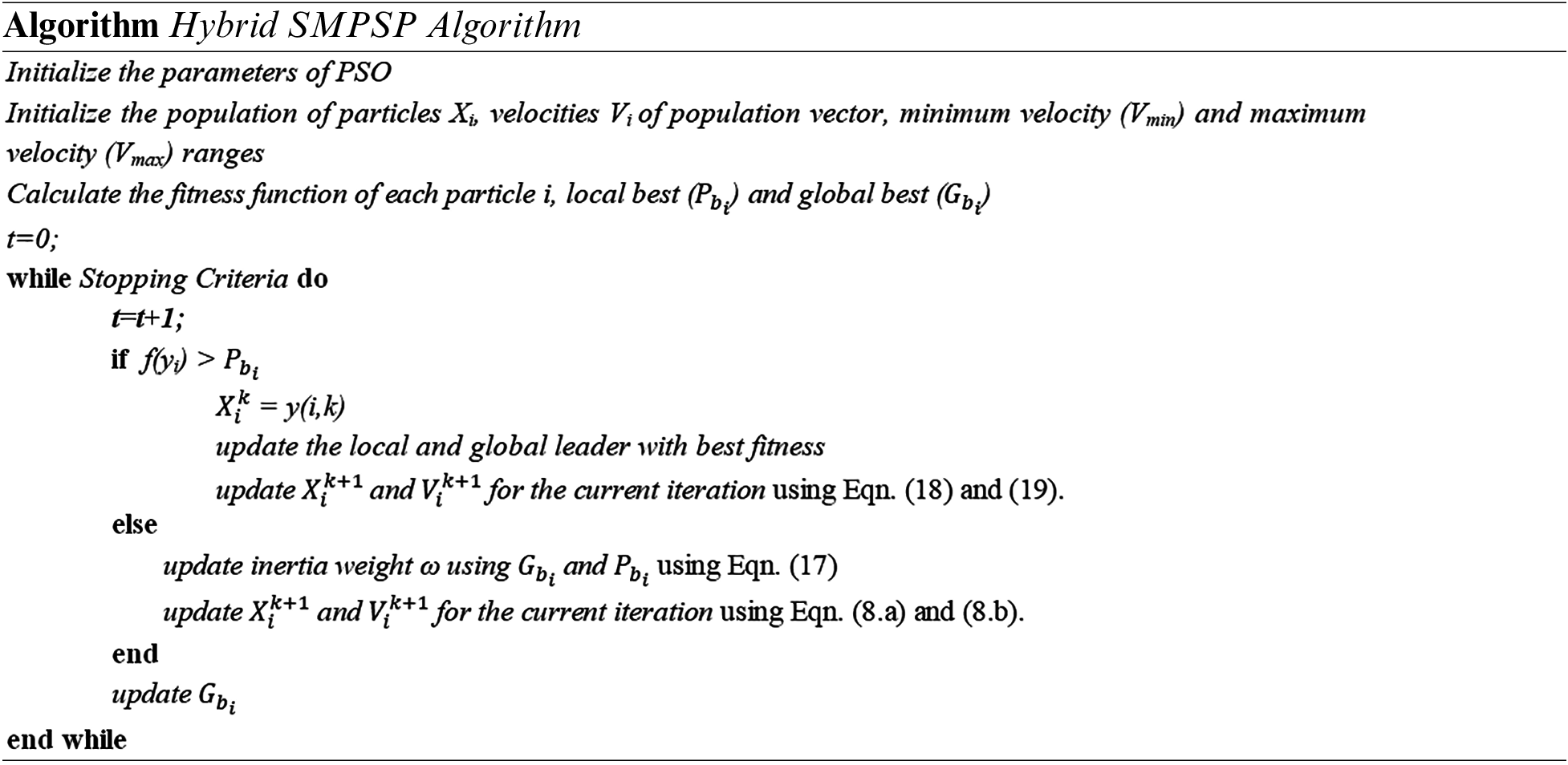
The primary objective of the hybrid Spider Monkey Particle Swarm Optimization (SMPSO) is to increase the Spider Monkey Optimizer’s exploration with Particle Swarm Optimization’s exploitation capabilities. It is a co-evolutionary technique since both techniques operate in parallel, not one after another. The first step is initializing each of PSO’s original parameters. Further the position and velocity of the population are randomly initialized within the predetermined ranges. The next step is calculating each particle’s fitness function, global best (Gbi) and local best (Pbi). After that, the fitness of the particle is evaluated with the current iteration to its previous iteration as per Eq. (16). If the fitness value is improved, the SMO algorithm will take over the other. Otherwise, the PSO algorithm continues following Eqs. (8.a) and (8.b) with the updated inertia weight ω in Eq. (17).

y(i,k+1)={true,if f(yi(k+1))>f(yi(k))false,if f(yi(k+1))≤f(yi(k))(16)

ω=(1.1−GbiPbi)(17)

If the SMO algorithm succeeds, the position and velocity of particle i is calculated with the local leader, global leader, and its own conscience according to Eqs. (18) and (19). All of the particles’ position and velocity ranges are updated and the algorithm will terminate with the optimum fitness value, and the final result will be the output.

Xik+1=Xik+U(0,1)×(Xik−GLmk)+U(0,1)×(Xrk−LLmk)(18)

Vik+1=Xik+1−Xik(19)

The proposed hybrid SMPSO algorithm pseudo-code is given below.

5  Image Dehazing Model Using Atrous Convolution-Based Residual Deep CNN

5.1 Atrous Convolution-Residual Deep CNN

In general, activation functions employed in convolution operations are typically utilized to extract the input data information by injecting a non-linearity into the network. The deep CNN uses 2D convolutional kernels which spans along the input image’s rows and columns and extract the features layer by layer. More feature maps will be extracted with the increase in layers, but at the expense of network complexity and training time. The deep learning model of atrous convolution-based residual deep CNN is shown in Fig. 4.

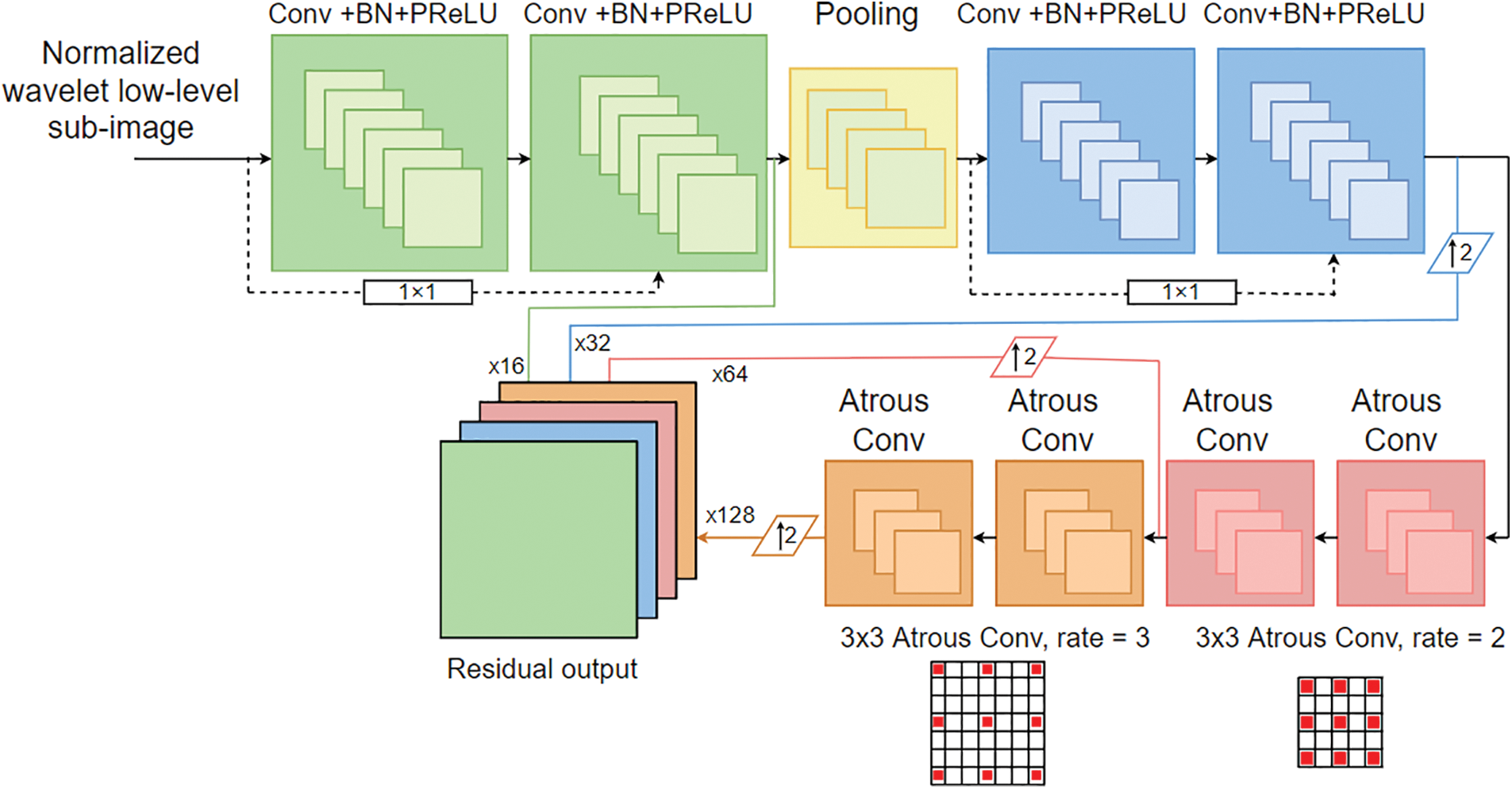
Figure 4: Deep learning model of atrous convolution-based residual deep CNN

The typical network architecture consists of four convolution layers designed with vanilla convolution, one max-pooling layer, four atrous convolution layers, concatenation of feature maps, residual connections, and skip connection. The Parametric REctified Linear Unit (PReLU) [40] activation function is used to combat the over-fitting and allow the network to learn more complex functions. The gradient descent algorithm used for this research is Stochastic Gradient Descent (SGD). The performance of the dehazing process is improved by maintaining the optimum batch size, epochs and the learning rate for more iterations using the hybrid SMPSO algorithm.

The feature maps will succeed from one layer to the next layer and convolve with the filter banks in the corresponding convolution layer. The response of each convolution layer is calculated using Eq. (20).

Vjl+1=f(∑iVil∗ki,jl+1+bijl+1)(20)

here, Vjl+1 and Vil are the respective feature maps of the (l + 1)th layer and lth layer, k is the 2D convolution kernel, ∗ denotes the convolution operator, i,j represents the current layer ith feature map to the next layer jth feature, f is the activation function and bnl+1 is the offset. The first shallow convolution layer (l = 1) learns the feature maps from the hazy input image.

The issue of overfitting occurs when there are fewer training samples than there are feature maps. To overcome this, PReLU activation function is used because of its superior convergence functionality than the Sigmoid and Tanh functions. The form of the PReLU activation function with learnable parameter zi as in Eq. (21). Max-pooling operation [41] further reduces the features resolutionand network parameters and maintains texture information of the image patch.

f(zi)=max(0,zi)+ai min(0,zi)(21)

The process of dehazing requires many feature maps to maintain the resolution. The latest U-Net [42] and 3D-Unet [43] utilize the convolution layers between features of different resolutions. This leads to a loss of feature representation which could not serve the purpose. A linear mapping using the shortcut connection with a convolution layer of size 1 × 1 increases the network training speed and combines features from different depths to communicate between the other resolutions. The features from different depths are concatenated to the final residual output.

The shallow convolutional layers of the network use a small receptive field to learn the short-range contextual information (local information). The deep atrous convolution layers use the larger receptive field to understand the long-range contextual information (global information). This enhances the extraction of contextual information. The global features of deep layers from different depths are propagated to the final output, resulting in a residual image. The atrous convolution kernel position can be expressed as in Eq. (22).

y(i)=∑jx(i+r⋅j)w[j](22)

here, x and y is are the respective layer input and output with a kernel w, i is the kernel position, and r is the dilation rate.

Every CNN model typically anticipates the normalized image before processing to reduce the dimensions and computational complexity. The normalized input images are split into patches, pooled in batches of size N, and sent to the CNN model. In the experiment, we chose the of 256 × 256 size input image patch to the network, and N = 50 as the batch size for training.

The shallow two vanilla convolution layers of the model are made up of 16 filters with stride equal to one with a kernel of 9 × 9. The max-pooling layer has a receptive field of 2 × 2. The second set of vanilla convolution layers of the model consists of 32 filters with a stride equal to one with kernel size 7 × 7. The deep atrous convolution layers consist of 64 filters and 128 filters with kernel sizes of 3 × 3 with a rate of 2 and 3 respectively. The network learns about 375,785 parameters in total from training.

5.2 Optimized Atrous Convolution-Based Residual Deep CNN

To enhance the dehazing performance of the atrous convolution-based residual deep CNN method, the hybrid SMPSO algorithm optimizes the batch size (B), epochs (E), and learning rate (L) with the objective function of optimum MSE and PSNR as in Eq. (23).

Obj=argminB,E,L(1PSNR)(23)

5.3 Loss Function

In recent image dehazing research, the different combinations of loss functions evolve endlessly to increase the image details. This increases the risk of tuning the hyper-parameters. After extensive testing, using a mean absolute error (MAE) function as in Eq. (24), as the loss function of our proposed method can have an apparent dehazing effect, as this function is sensitive to sparse features of the input image.

LossMAE=1CWH∑m∑n∑p||Z^m,n,p−Zm,n,p||(24)

here, Z^m,n,p represents the recovered haze-free image, and Zm,np represents the corresponding ground truth training label, C,W,H denotes the channel count, width and height of the training image respectively.

6  Results and Discussions

6.1 Experimental Setup

The proposed image dehazing framework requires TensorFlow deep learning framework. The optimized batch size is 48 and 44; optimum number of epochs is 75 and 62; the optimum learning rate is 0.84 and 0.76 for corresponding datasets. The network training and evaluation are performed in a server with a personal computer, 16 GB RAM, Intel® Core i7-1280P Processor, and NVIDIA Graphical Processing Unit to speed up the network operation. The network is subjected to critical training and reconstruction constraints.

6.2 Performance Metrics

The performance assessment metrics used for analysis in this research work are Mean Square Error (MSE), Peak Signal to Noise Ratio (PSNR), Mean Absolute Error (MAE), Average Difference (AD), and Maximum Difference (MD) and Structural Similarity Index (SSIM).

(a)   Mean Square Error (MSE): It is a dispersion metric for measuring the efficiency of image enhancement algorithms in the applications of real-world image processing. It is measured as the difference among the recovered clear image and the corresponding ground truth image as in Eq. (25).

(b)   Peak Signal to Noise Ratio (PSNR): It is a higher order and correlative metric depending on MSE used to measure the quality of the recovered clear image as in Eq. (26).

(c)   Mean Absolute Error (MAE): It is a conventional metric to measure the amount of haze effect present in an input image as in Eq. (27).

(d)   Average Difference (AD): It is widely used in image processing applications including object detection and recognition. It is the average concern pixel change in the recovered image and its respective ground truth image as in Eq. (28).

(e)   Maximum Difference (MD): It is the maximum of the absolute difference among the recovered image and its respective ground truth image as in Eq. (29).

(f)   Structural Similarity Index Metric (SSIM): It is a higher order metric used to assess the quality of the dehazed image concerning ground truth image as in Eq. (30), typically its value lies from 0 to 1.

The expressions for the above metrics are provided below

MSE=1MN∑m=1M∑n=1N(D(m,n)−G(m,n))2(25)

PSNR=10log10⁡Imax2MSE(26)

MD=|D(m,n)−G(m,n)|(27)

MAE=1MN∑m=1M∑n=1N|D(m,n)−G(m,n)|(28)

AD=1MN∑m=1M∑m=1N(D(m,n)−G(m,n))(29)

here, D and G are the dehazed and corresponding hazy input image at location m,n coordinates with a pixel count of M × N along the horizontal and vertical directions respectively, Imax is the maximum possible intensity, typically it is set to 255

SSIM=(2μmμn+C1)(σmn+C2)(μm2+μn2+C1)(σm2+σn2+C2)(30)

here, μm, μn is the average of m,n, σm,σn is the standard deviation of m,n, σmn is the covariance of  m,n and C1, C2 are set constants to avoid any possibility of the denominator being zero.

6.3 Statistical Analysis of Atrous-Deep CNN with Optimization Algorithms

The recovered clear images obtained using CNN [21], MSCNN [24], Ranking CNN [44], Deep CA learning [45], Autoencoder [46], and the proposed method with an optimization algorithm, are depicted in Fig. 5 for respective datasets.

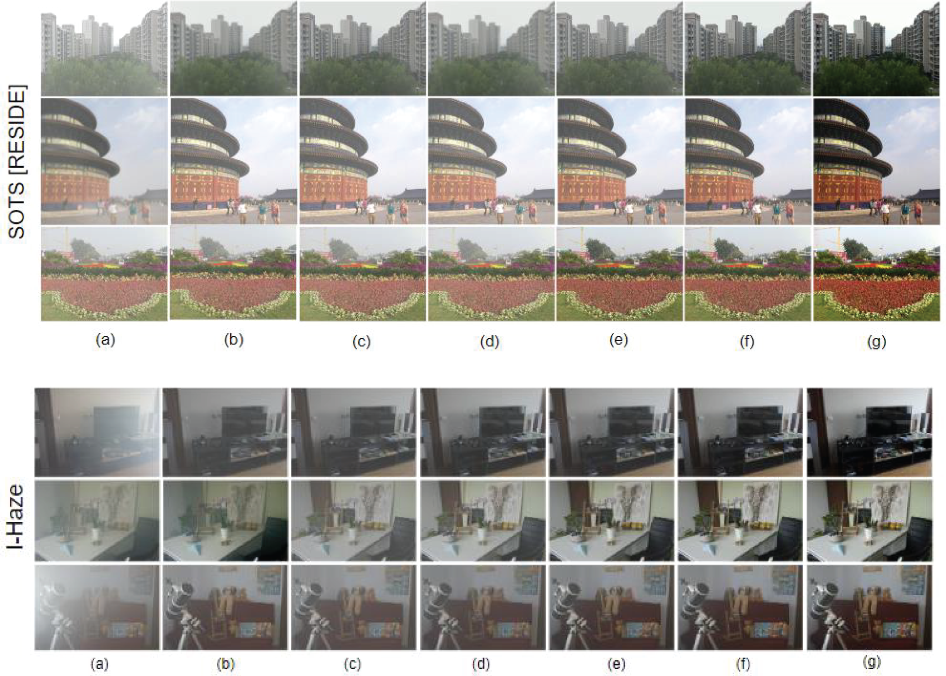
Figure 5: Dehazed images using (a) Haze input (b) CNN [21] (c) MSCNN [24] (d) Ranking CNN [44] (e) DeepCA learning [45] (f) Autoencoder [46] (g) Proposed deep learning network

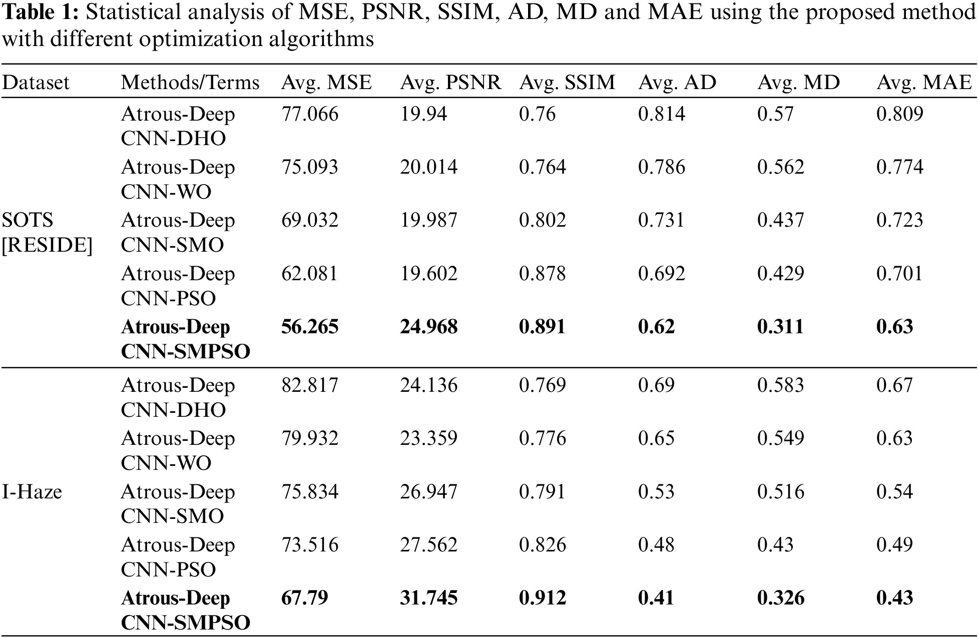
The statistical analysis of MSE, PSNR, SSIM, AD, MD, and MAE using proposed atrous convolution-based deep CNN with Deer Hunting Optimization (DHO) [47], Whale Optimization (WO) [48], SMO [39], PSO [38] and newly designed hybrid SMPSO algorithm on the respective datasets is shown in Table 1.

The analysis of MSE and PSNR for existing methods and the proposed method with hybrid SMPSO algorithm on the respective datasets are shown in Table 2 and the analysis of SSIM, MAE, AD and MD is shown in Fig. 6. The optimized solutions of meta-heuristic algorithms on the proposed method are shown in Table 3.

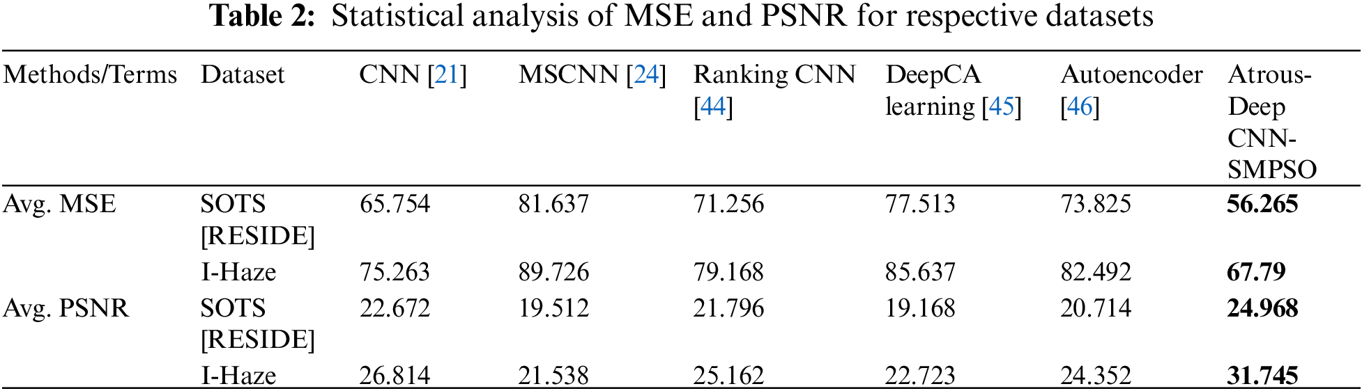
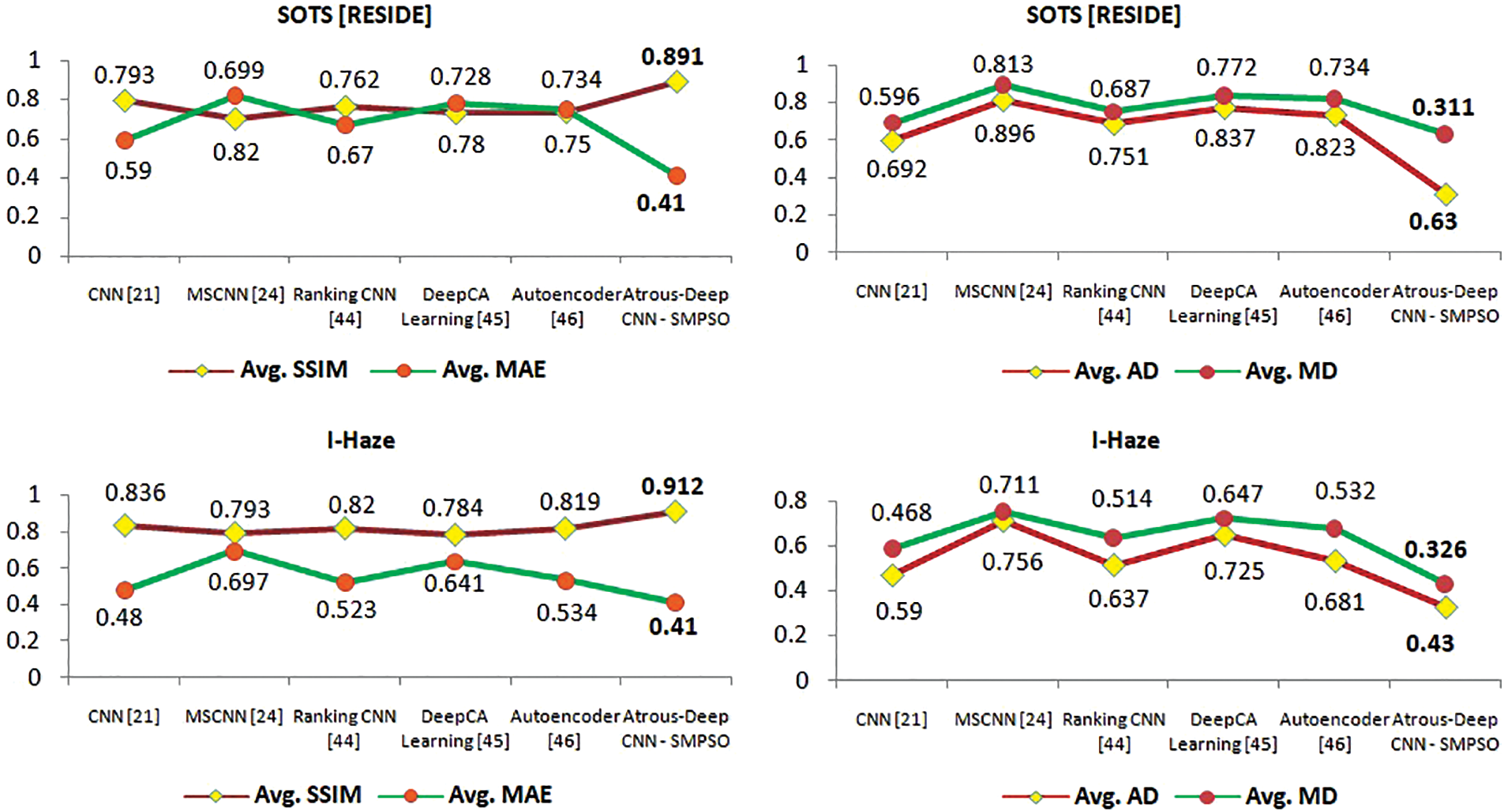
Figure 6: Statistical analysis of SSIM, MAE, AD and MD on existing methods and proposed method

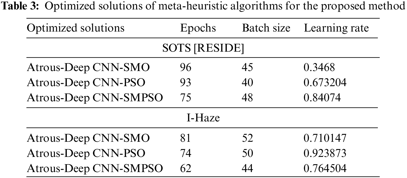
The statistical analysis in Tables 1 and 2 shows that the proposed atrous convolution-based hybrid SMPSO algorithm performs better than other optimization algorithms and existing methods respectively. Table 3 shows that the optimum values of no. of epochs, batch size and the learning rate areobtained with a proposed method with a hybrid optimization algorithm.

The proposed atrous convolution extracts the full range of contextual information from the low-frequency wavelet decomposed images. These reduces the number of convolution layers during network training and enhances the efficiency of the network in dehazing process. The results obtained shows the qualitative and quantitative performance of the proposed method with the optimum batch size, epochs and learning rate using hybrid optimization.

7  Conclusion

In this article, we propose an optimized atrous convolution-based Deep CNN using a hybrid SMPSO algorithm for image dehazing without relying on atmospheric scattering models. This method generates a clean image free from halo artifacts and poor contrast. The wavelets provide extensive features useful for deep learning models and have high-performance achieving capabilities. The proposed Deep CNN model uses the wavelet multi-resolution features for training, to estimate the extent of the haze effect and predict the clear image from the haze patches. The hybrid optimization algorithm is designed to fine-tune the batch size, epochs, and learning rate required during the data model training. The designed atrous-deep CNN network inherits the local and higher-order features using atrous convolution and residual connection. The experimental analysis has proven the outstanding performance of the proposed method and quantitative metrics like MSE, PSNR, SSIM, MAE, AD, and MD have been considerably improved with existing optimization algorithms and deep learning methods. The method further can be extended to real-world aerial hazy datasets in change detection, image segmentation tasks, hazy video surveillance tasks and the network model can be strengthened by optimizing more parameters for accurate estimation of the image scenes.

Acknowledgement: We would like to thank the Management for providing the NVIDIA GPU support to train the proposed neural network for analysis.

Funding Statement: The authors received no specific funding for this study.

Conflicts of Interest: The authors declare that they have no conflicts of interest to report regarding the present study.

References

1. J. Kopf, B. Neubert, B. Chen, M. Cohen, D. Cohen-Or et al., “Deep photo: Model-based photograph enhancement and viewing,” ACM Transactions on Graphics, vol. 27, no. 5, pp. 1–10, 2008. [Google Scholar]

2. T. Treibitz and Y. Y. Schechner, “Polarization: Beneficial for visibility enhancement?” in 2009 IEEE Conf. on Computer Vision and Pattern Recognition, Miami, FL, USA, pp. 525–532, 2009. [Google Scholar]

3. L. P. Yao and Z. I. Pan, “The retinex-based image dehazing using a particle swarm optimization method,” Multimedia Tools and Applications, vol. 80, no. 3, pp. 3425–3442, 2021. [Google Scholar]

4. C. M. S. Kumar, R. S. Valarmathi and S. Aswath, “An empirical review on image dehazing techniques for change detection of land cover,” in 2021 Asian Conf. on Innovation in Technology (ASIANCON), Pune, India, pp. 1–9, 2021. [Google Scholar]

5. K. He, J. Sun and X. Tang, “Single image haze removal using dark channel prior,” in 2009 IEEE Conf. on Computer Vision and Pattern Recognition, Miami, FL, USA, pp. 1956–1963, 2009. [Google Scholar]

6. D. Berman, T. Treibitz and S. Avidan, “Air-light estimation using haze-lines,” in 2017 IEEE Int. Conf. on Computational Photography (ICCP), Stanford, CA, USA, pp. 1–9, 2017. [Google Scholar]

7. Q. Zhu, J. Mai and L. Shao, “A fast single image haze removal algorithm using color attenuation prior,” IEEE Transactions on Image Processing, vol. 24, no. 11, pp. 3522–3533, 2015. [Google Scholar] [PubMed]

8. L. Peng and B. Li, “Single image dehazing based on improved dark channel prior and unsharp masking algorithm,” in Intelligent Computing Theories and Application, ICIC 2018, Wuhan, China, vol. 10954, pp. 347–358, 2018. [Google Scholar]

9. D. Singh, V. Kumar and M. Kaur, “Single image dehazing using gradient channel prior,” Appllied Intelligence, vol. 49, no. 12, pp. 4276–4293, 2019. [Google Scholar]

10. B. Cai, X. Xu, K. Jia, C. Qing and D. Tao, “DehazeNet: An end-to-end system for single image haze removal,” IEEE Transactions on Image Processing, vol. 25, no. 11, pp. 5187–5198, 2016. [Google Scholar]

11. W. -Y. Hsu and Y. -S. Chen, “Single image dehazing using wavelet-based haze-lines and denoising,” IEEE Access, vol. 9, pp. 104547–104559, 2021. https://doi.org/10.1109/ACCESS.2021.3099224 [Google Scholar] [CrossRef]

12. S. G. Narasimhan and S. K. Nayar, “Contrast restoration of weather degraded images,” IEEE Transactions on Pattern Analysis and Machine Intelligence, vol. 25, no. 6, pp. 713–724, 2003. [Google Scholar]

13. D. Singh and V. Kumar, “A novel dehazing model for remote sensing images,” Computers & Electrical Engineering, vol. 69, pp. 14–27, 2018. https://doi.org/10.1016/j.compeleceng.2018.05.015 [Google Scholar] [CrossRef]

14. C. Li, J. Guo, F. Porikli, H. Fu and Y. Pang, “A cascaded convolutional neural network for single image dehazing,” IEEE Access, vol. 6, pp. 24877–24887, 2018. https://doi.org/10.1109/ACCESS.2018.2818882 [Google Scholar] [CrossRef]

15. Y. Liu, J. Shang, L. Pan, A. Wang and M. Wang, “A unified variational model for single image dehazing,” IEEE Access, vol. 7, pp. 15722–15736, 2019. https://doi.org/10.1109/ACCESS.2019.2894525 [Google Scholar] [CrossRef]

16. H. Zhang and V. M. Patel, “Densely connected pyramid dehazing network,” in 2018 IEEE/CVF Conf. on Computer Vision and Pattern Recognition, Salt Lake City, UT, USA, pp. 3194–3203, 2018. [Google Scholar]

17. Y. Y. Schechner, S. G. Narasimhan and S. K. Nayar, “Polarization-based vision through haze,” Applied Optics, vol. 42, no. 3, pp. 511–525, 2003. [Google Scholar] [PubMed]

18. Z. Mi, H. Zhou, Y. Zheng and M. Wang, “Single image dehazing via multiscale gradient domain contrast enhancement,” IET Image Processing, vol. 10, no. 3, pp. 206–214, 2016. [Google Scholar]

19. Y. Wan and Q. Chen, “Joint image dehazing and contrast enhancement using the HSV color space,” in 2015 Visual Communications and Image Processing (VCIP), Singapore, pp. 1–4, 2015. [Google Scholar]

20. C. O. Ancuti and C. Ancuti, “Single image dehazing by multi-scale fusion,” IEEE Transactions on Image Processing, vol. 22, no. 8, pp. 3271–3282, 2013. [Google Scholar] [PubMed]

21. J. Li, G. Li and H. Fan, “Image dehazing using residual-based deep CNN,” IEEE Access, vol. 6, pp. 26831–26842, 2018. https://doi.org/10.1109/ACCESS.2018.2833888 [Google Scholar] [CrossRef]

22. Z. Li, B. Gui, T. Zhen and Y. Zhu, “Grain depot image dehazing via quadtree decomposition and convolutional neural networks,” Alexandria Engineering Journal, vol. 59, no. 3, pp. 1463–1472, 2020. [Google Scholar]

23. Z. Liu, B. Xiao, M. Alrabeiah, K. Wang and J. Chen, “Single image dehazing with a generic model-agnostic convolutional neural network,” IEEE Signal Processing Letters, vol. 26, no. 6, pp. 833–837, 2019. [Google Scholar]

24. W. Ren, J. Pan, H. Zhang, X. Cao and M. yang, “Single image dehazing via multi-scale convolutional neural networks with holistic edges,” International Journal of Computer Vision, vol. 128, pp. 240–259, 2020. https://doi.org/10.1007/s11263-019-01235-8 [Google Scholar] [CrossRef]

25. K. Gan, J. Zhao and H. Chen, “Multilevel image dehazing algorithm using conditional generative adversarial networks,” IEEE Access, vol. 8, pp. 55221–55229, 2020. https://doi.org/10.1109/ACCESS.2020.2981944 [Google Scholar] [CrossRef]

26. S. Zhang and F. He, “DRCDN: Learning deep residual convolutional dehazing networks,” The Visual Computer, vol. 36, no. 9, pp. 1797–1808, 2020. [Google Scholar]

27. S. Wang, L. Zhang and X. Wang, “Single image haze removal via attention-based transmission estimation and classification fusion network,” Neurocomputing, vol. 447, pp. 48–63, 2021. [Google Scholar]

28. F. A. Dharejo, Y. Zhou, F. Deeba, M. A. Jatoi, M. A. Khan et al., “A deep hybrid neural network for single image dehazing via wavelet transform,” Optik, vol. 231, pp. 166462, 2021. https://doi.org/10.1016/j.ijleo.2021.166462 [Google Scholar] [CrossRef]

29. D. Yang and J. Sun, “A Model-driven deep dehazing approach by learning deep priors,” IEEE Access, vol. 9, pp. 108542–108556, 2021. https://doi.org/10.1109/ACCESS.2021.3101319 [Google Scholar] [CrossRef]

30. C. Wang, Z. Li, J. Wu, H. Fan, G. Xiao et al., “Deep residual haze network for image dehazing and deraining,” IEEE Access, vol. 8, pp. 9488–9500, 2020. https://doi.org/10.1109/ACCESS.2020.2964271 [Google Scholar] [CrossRef]

31. X. Min, G. Zhai, K. Gu, Y. Zhu, J. Zhou et al., “Quality evaluation of image dehazing methods using synthetic hazy images,” IEEE Transactions on Multimedia, vol. 21, no. 9, pp. 2319–2333, 2019. https://doi.org/10.1109/TMM.2019.2902097 [Google Scholar] [CrossRef]

32. T. Yu, M. Zhu and H. Chen, “Single image dehazing based on multi-scale segmentation and deep learning,” Machine Vision and Applications, vol. 33, no. 2, pp. 1–11, 2022. [Google Scholar]

33. A. Bilal, G. Sun and S. Mazhar, “Diabetic retinopathy detection using weighted filters and classification using CNN,” in Proc. of 2021 Int. Conf. on Intelligent Technologies (CONIT), Hubli, India, pp. 25–27, 2021. [Google Scholar]

34. A. Bilal, G. Sun, Y. Li, S. Mazhar and J. Latif, “Lung nodules detection using grey wolf optimization by weighted filters and classification using CNN,” Journal of the Chinese Institute of Engineers, vol. 45, no. 2, pp. 175–186, 2022. [Google Scholar]

35. D. L. Donoho and I. M. Johnstone, “Ideal spatial adaptation by wavelet shrinkage,” Biometrika, vol. 81, no. 3, pp. 425–455, 1994. [Google Scholar]

36. C. Blum, M. J. B. Aguilera, A. Roli and M. Sampels, “Hybrid metaheuristics,” in An Emerging Approach to Optimization, Heidelberg: Springer Berlin, 2008. https://doi.org/10.1007/978-3-540-78295-7 [Google Scholar] [CrossRef]

37. R. Poli, J. Kennedy and T. Blackwell, “Particle swarm optimization,” Swarm Intelligence, vol. 1, pp. 33–57, 2007. https://doi.org/10.1007/s11721-007-0002-0 [Google Scholar] [CrossRef]

38. Y. Shi and R. Eberhart, “A modified particle swarm optimizer,” in 1998 IEEE Int. Conf. on Evolutionary Computation Proc. IEEE World Congress on Computational Intelligence, Anchorage, AK, USA, pp. 69–73, 1998. [Google Scholar]

39. J. C. Bansal, H. Sharma, S. S. Jadon and M. Clerc, “Spider monkey optimization algorithm for numerical optimization,” Memetic Computing, vol. 6, pp. 31–47, 2014. https://doi.org/10.1007/s12293-013-0128-0 [Google Scholar] [CrossRef]

40. R. S. Thakur, R. N. Yadav and L. Gupta, “PReLU and edge-aware filter-based image denoiser using convolutional neural network,” IET Image Process, vol. 14, pp. 3869–3879, 2020. https://doi.org/10.1049/iet-ipr.2020.0717 [Google Scholar] [CrossRef]

41. Z. Zuo, B. Shuai, G. Wang, X. Liu, X. Wang et al., “Learning contextual dependence with convolutional hierarchical recurrent neural networks,” IEEE Transactions on Image Processing, vol. 25, no. 7, pp. 2983–2996, 2016. [Google Scholar] [PubMed]

42. O. Ronneberger, P. Fischer and T. Brox, “U-Net: Convolutional networks for biomedical image segmentation,” Medical Image Computing and Computer-Assisted Intervention–MICCAI 2015, Lecture Notes in Computer Science, vol. 9351, 2015. https://doi.org/10.1007/978-3-319-24574-4_28 [Google Scholar] [CrossRef]

43. K. Kamnitsas, C. Ledig, V. F. J. Newcombe, J. P. Simpson, A. D. Kane et al., “Efficient multi-scale 3D CNN with fully connected CRF for accurate brain lesion segmentation,” Medical Image Analysis, vol. 36, pp. 61–78, 2017. https://doi.org/10.1016/j.media.2016.10.004 [Google Scholar] [PubMed] [CrossRef]

44. Y. Song, J. Li, X. Wang and X. Chen, “Single image dehazing using ranking convolutional neural network,” IEEE Transactions on Multimedia, vol. 20, no. 6, pp. 1548–1560, 2018. [Google Scholar]

45. S. Tangsakul and S. Wongthanavasu, “Single image haze removal using deep cellular automata learning,” IEEE Access, vol. 8, pp. 103181–103199, 2020. https://doi.org/10.1109/ACCESS.2020.2999076 [Google Scholar] [CrossRef]

46. G. Kim, S. W. Park and J. Kwon, “Pixel-wise wasserstein autoencoder for highly generative dehazing,” IEEE Transactions on Image Processing, vol. 30, pp. 5452–5462, 2021. https://doi.org/10.1109/TIP.2021.3084743 [Google Scholar] [PubMed] [CrossRef]

47. P. Durgaprasadarao and N. Siddaiah, “Design of deer hunting optimization algorithm for accurate 3D indoor node localization,” Evolutionary Intelligence, 2021. https://doi.org/10.1007/s12065-021-00673-z [Google Scholar] [CrossRef]

48. J. Rahebi, “Vector quantization using whale optimization algorithm for digital image compression,” Multimedia Tools and Applications, vol. 81, pp. 20077–20103, 2022. https://doi.org/10.1007/s11042-022-11952-x [Google Scholar] [CrossRef]