Noise-Filtering Enhanced Deep Cognitive Diagnosis Model for Latent Skill Discovering

1  Introduction

Personalized education for students’ characteristics in the context of big data in education in order to realize teaching according to their abilities is an important direction of current research on smart education. The rapid development of online education and major online learning platforms in recent years has promoted the large-scale popularity of online learning [1–3]. With the increasing abundance of learning resources in online learning platforms, it has become increasingly important to provide personalized learning services for students. Based on students’ online learning data, it is an important research hotspot to analyze students’ learning status by means of educational data mining (EDM) technology and make accurate recommendations for personalized learning based on students’ actual characteristics in order to realize teaching based on their abilities [4–8]. In order to achieve personalized learning guidance for students, it is first necessary to identify the current learning status of students [9–12]. Traditional teaching methods rely on teachers’ experience to make judgments, which not only takes a lot of time and energy, but also makes it difficult to guarantee the accuracy of evaluation results, and is not suitable for application scenarios where the size of students increases dramatically in the online learning environment [13–15].

To this end, the researcher attempted to introduce the cognitive diagnosis (CD) method in educational psychology to characterize students’ learning status [16–18]. The key to cognitive diagnosis is to construct a Q matrix reflecting students’ problem solving process and to choose appropriate cognitive diagnostic models (CD models) to model students [19,20]. The cognitive diagnostic model (CDM) [21,22] is an important tool for achieving cognitive diagnosis, and an increasing number of researchers have worked on the development of this model. The traditional CDM uses different item response functions to probabilistically model students’ response processes through different learning assumptions to diagnose their skill mastery status [23,24]. However, traditional CDM has some problems, such as the convergence effect of the model is highly dependent on the sample size, number of skills and number of parameters, which cannot handle sparse data, and it is difficult to explore the potential nonlinear interactions between students and test questions.

With the gradual development of computer technology, deep learning techniques excel in many aspects, such as mining non-linear aspects of interactions and handling sparse data [22–24]. Therefore, some scholars have attempted to incorporate neural networks into cognitive diagnosis tasks to improve the model fitting ability. The study [25] proposed the DIRT model, which implements a neural network-based IRT model that can utilize textual information from examination questions in the cognitive diagnosis process. Study [26] proposed the neural CD model, which combines neural networks with the principle of educational monotonicity and achieves excellent performance on various data sets with good portability. However, in the combination of cognitive diagnostics with neural networks, a large amount of research work has focused more on improving the predictive ability of students’ correct answers without deeply exploring the intermediate products of CD (e.g., students’ skill mastery status) to achieve CD functionality. Therefore, the existing deep cognitive diagnostics, although improving the model fitting ability, cannot better model students’ cognitive processes and lack good explanatory power.

Based on the above research, this paper proposes a two-level enhancement model that integrates deep learning and cognitive diagnosis to diagnostic students’ skill mastery states. On the one hand, the advantages of CDM are used to enhance the interpretability of the models. On the other hand, the unique technical advantages of the deep learning method itself can mine the non-linear relationship between students’ skill states and test questions, and to a certain extent can solve the problem that sparse data is difficult to be used by the model. Based on the combination of the both, not only the interpretability of the model can be improved, but also the accuracy of the model can be improved by mining the non-linear interaction data between students and test questions.

The main contributions of this paper are as follows:

1) We propose an innovative cognitive diagnostic framework based on deep learning for uncovering students’ potential skill mastery status. The model is divided into three modules: enhanced input module, deep training module, and prediction module.

2) By modelling the interaction between student-skills (i.e., student skill mastery) and questions-skills (i.e., Q matrix), we obtain students’ question proficiency and further apply filtering network mechanisms to filter noise, such as guessing and slipping, to enhance the interpretability of the model.

3) The neural network is further used to simulate the cognitive process of the students’ responses to the questions, and to train the students skill mastery by predicting the results of their responses. The method uses multiple neurons to model the non-linear interaction between students and questions, improving the fitting ability of traditional models.

2  Background Knowledge

In this section, we discuss the research related to Traditional CDM and Deep CDM, and compare the two modeling approaches, as shown in Fig. 1. Among them, the Traditional CDM is to model the interaction between students and test questions through manually constructed item response functions; Deep CDN is capable of mining richer information by modeling the complex interactions between students and test questions through neural network.

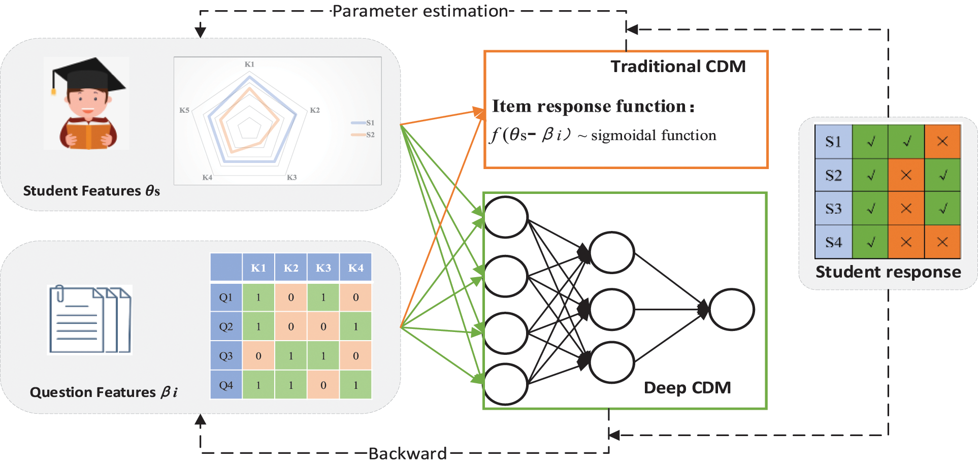
Figure 1: Comparison of cognitive diagnostic modeling approaches

2.1 Traditional CDM

Traditional CDMs model the interaction between students and test questions by constructing item response functions using probabilistic statistical models through the monotonicity assumption that the more skills a student examines on a test question, the greater the probability of answering the question correctly. IRT is a classic psychometric theory in the field of education and a representative of the continuum-type of CD model. It is assumed that the subject has a potential trait, which is a concept based on the observation and analysis of the subject’s responses, usually referring to potential abilities. In a continuum-type model based on IRT, students’ potential traits are generally modeled along a continuum of values. IRT proposed the earliest Rasch model [9]. With consideration of how to define both the ability of the subject and the difficulty of the test questions, the item response function is defined follow:

P(y=1/θ,δi)=exp⁡(θ−δi)/[1+exp⁡(θ−δi)](1)

where P(y=1/θ,δi) is the probability that a subject with ability θ will answer a question of difficulty δi correctly (y=1).

CDMs can better model students’ cognitive states from the skill dimension, based on the Q matrix [10]. Among the existing CD models, the DINA model has been most extensively studied. The DINA model is representative of discrete CD models [11]. It treats students’ cognitive state as a binary discrete vector, with two dimensions indicating students’ mastery or non-mastery of the relevant knowledge concepts, and usually assumes an ‘and’ relationship between the mastery of each knowledge concept, the item response function is constructed:

P(yij=1|θi)=gj1−ηij(1−sj)ηij(2)

where ηij∈{0,1} indicates student I’s mastery of test question j, ηij=1 indicates that student i has mastered all the knowledge points examined in test question j, otherwise ηij=0; sj is the error parameter of question j, which indicates the probability that the student has mastered all the examined knowledge points but answered incorrectly; gj is the guessing factor of question j, which indicates the probability that the student has not mastered test j and guessed incorrectly.

2.2 Deep CDM

The study [27] proposed the definition of Deep Cognitive Diagnostic Model (DCDM), which is the use of deep learning techniques to enhance the cognitive diagnostic capabilities of traditional cognitive diagnostic models. The study [28] applied rough sets and neural networks to psychometric theory. Study [29] used cluster analysis for CD. However, in the integration of cognitive diagnoses with neural networks, many research efforts have focused more on improving the predictive ability of students’ correct answers without an in-depth exploration of the intermediate product of cognitive diagnoses (e.g., students’ skill mastery status). In conclusion, the current deep CDM has made some advancements in simulating non-linear interactions and improving model fit, but it lacks interpretability and does not allow for the diagnosis of student skill mastery.

The difficulty of deep CD is its widely criticized black box nature, i.e., the model parameters are difficult to interpret. The CD needs to get the students’ level of mastery on each knowledge point, so this is the hurdle that must be crossed. Meanwhile, neural networks also present new opportunities, as their powerful fitting abilities allow their CDM to learn more complex and realistic interaction functions from the data. This research proposes a model that integrates deep learning with CD the goal of diagnosing students’ skill states.

3  Method

The existing DCDM has weak diagnostic ability in the state of students’ skill mastery, and lacks interpretation. In this section, we propose a two-level enhanced deep cognitive diagnosis (EDCD) model based on deep learning for mining students’ skill mastery. The EDCDM framework, as shown in Fig. 2, mainly includes input module, training module and prediction module.

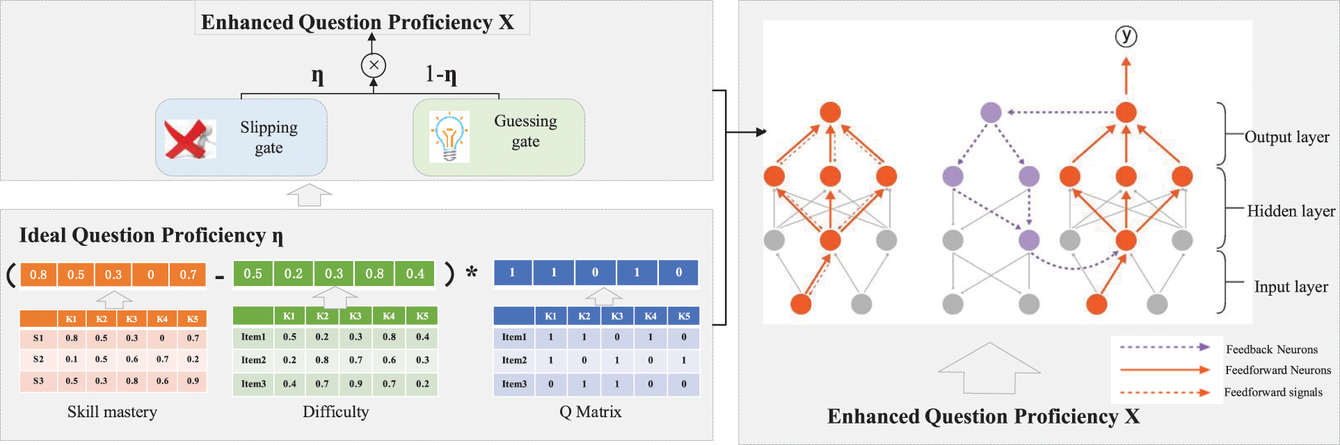
Figure 2: Two-level enhanced deep cognitive diagnosis framework

3.1 Problem Definition

The main task of the initialization module is to randomly initialize the generated parameters for use in the two-level optimization input module. The parameters are taken from the traditional CDMs and represented in the neural network in the form of appropriate data. It is assumed that there are J test questions examining K skills, answered by student I.

Question features: matrix Q={qjk}J×K is the association matrix between test questions and skills, qjk=1 indicating that test question j examines skill k, qjk=0 indicating that test question j does not examine skill k. The initialized questions’ difficulty matrix K={kjk}j×K, kjk∈[0,1] indicates the difficulty factor of applying skill K in question J.

Student features: αi={αik} initialize the skill mastery pattern of student i, αik∈[0,1] indicating the mastery status of student i for skill k. Student response matrix Yi={yij}I×j, yij=1 indicating that student i answered question j correctly, otherwise yij=0.

Monotonicity Assumption: The probability of students correctly answering the questions increases monotonously with the student’s skill mastery.

Here the parameters are initialized in the form of a tensor parameter. Initialize the continuous mastery of each skill for each student. Such an initialization pattern provides a wider correction space for the inverse feedback iteration and brings the student’s skill mastery closer to the true value.

3.2 Enhanced Input Module

This input module obtains students’ question proficiency through a two-layer mechanism: the first layer is the ideal state; the second layer is for filtering noise. The main function of the two-level enhanced input module, shown in Fig. 2 (left), is to combine various randomly generated parameters in the form of DINA formulas by Eq. (2) and then provide the results as input to the next module.

First layer: The first layer obtains the ideal question proficiency state of the students by αi and Q matrix. We confront the knowledge points mastered by the i student with the relevant skills of the j-question test to obtain ηij=(αi−kj)∗qj, among others, the expert labeling qj matrix to mark the corresponding skills of the question test with the values of [0,1].

Second layer: A Slipping gate (sj) and a guessing gate (gj) are added to the second layer to filter the mastery status of students on the questions. Two parameter vectors, SLIP and GUESS, are randomly initialized to represent the lapse parameters and guess parameters of students, respectively. The slip gate mechanism S=[s1,s2,…,sj] is set to prevent students from mastering the skills of the test questions but making mistakes, and the guess gate mechanism G=[g1,g2,…,gj] is set to prevent students from not mastering the skills of the test questions but guessing the correct answers. The input matrix X is obtained by setting the miss gate and the guessers to optimize the mastery status of the test student.

X=(1−sj)ηijgj1−ηij(3)

The parameter ηij ∈ [0,1] indicates the degree of mastery of question j by the student i. sj is the slip gate, which filters the cases where the student still answers incorrectly when he/she has mastered all the skills required for the question. gj is the guessing gate, which filters the cases when the student has failed to fully master all the knowledge points required for the question, but still answered correctly. The two-gate mechanism enhances the fit to the student’ mastery of the knowledge points.

3.3 Deep Training Module

The core of EDCDM is to use the parameter updating mechanism of neural networks to bring the involved parameters closer to the true values by adjusting the mapping relationship between inputs and outputs. Then the continuous predicted values of potential features (such as the student’ skill mastery) are obtained, and the predicted values gradually approach the potential true values, and the prediction accuracy gradually improves.

3.3.1 Neural Network Structure

This section combines the information of two dimensions, test question difficulty and student mastery, and after receiving the mixed input X, X will be transferred to the first fully connected layer (Linear layer). X1 is obtained by linear mapping in the first fully connected layer and then processed by sigmoid activation function. Then the transfer X1 goes to the second fully connected layer and the above steps are repeated. After repeating the linear-sigmoid process twice, we obtain the mapping product X2. The equation is described as follows.

zi=wijτXi+bi(4)

Xi+1=sigmoid(zi)(5)

We use a splicing technique between the second linear-sigmoid layer and the third linear-sigmoid layer to splice the mapping product X2 and the mixed input X into the third linear-sigmoid layer. X3 is the output product of the output side of the neural network, and the loss calculation is performed directly with the real student answer record y by the Eq. (6).

3.3.2 Prediction Module

This paper uses a method to calculate the error gradient under each weight in real time. It is a classical method for training neural networks in combination with optimization methods (such as gradient descent, etc.) and consists of two parts: incentive propagation and weight update. In the incentive propagation phase, each iteration is performed in two steps:

1)   Input the training results into the network to obtain the excitation response;

2)   Differentiate the excitation response from the corresponding output target to obtain the response error of the output and hidden layers.

In the weight update phase, two steps are performed for each weight:

1)   Multiply the input excitation and response errors to obtain the gradient of the weights;

2)   Use this gradient to multiply the learning rate, then take its inverse and add it to the weights.

In this model, the parameter update mechanism plays the role of updating the parameters for fitting, as described by the following equation.

ΔWij=−λ∂E∂Wij=−λXiδj(6)

where, E∑i=03⁡12(y−Xi)2 is the mean square error term of the three connecting layers. The variables Wij denote the neuron weights between i and j, defined ΔWij as the weight update, λ is the learning rate, and ∂E∂Wij denotes the partial derivative of the squared error function. Xi is the output of the current neuron, and δj is the error generated by neuron j in the current layer (i.e., the error between the actual value and the predicted value). The input Xi to neuron j is partially obtained from the weighted sum of the outputs Xi of neuron I in the upper layer.

In the structure of the feedback neural network, this model chooses the Cross Entropy Loss Function (CELF) as the loss function to measure the loss between the predicted and true values, and proves the validity of the model by pursuing a lower loss value. The CELF equation can be defined as Eq. (9).

P(rij=1∣θi)=y^(7)

P(rij=0∣θi)=1−y^(8)

lossDCDM=−∑i=13y(i)log⁡y^(i)+(1−y(i))log⁡(1−y^(i))(9)

The deep diagnosis module builds on the first two by using a good fit of the neural network to predict the probability of the correct answer of the student by the Eqs. (8) and (9). In this process, rich intermediate results can be obtained due to the rational use of inverse feedback. For example, the degree of the student’s mastery of a specific skill, the difficulty of the knowledge point in the exam test, etc. Such intermediate findings are a useful complement to cognitive diagnosis.

4  Experiment

In this section, we conduct several experiments to demonstrate the effectiveness of the EDCDM framework from multiple perspectives, using multiple datasets and comparing them to the baseline model.

4.1 Datasets

We used three real-world datasets in our experiments, namely PISA 2015 [4], Math [5], and Assist [6]. Table 1 summarizes the information from these datasets.

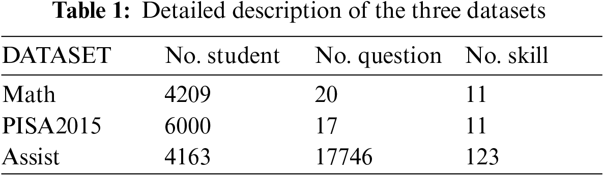
Math: The Math dataset is a dataset of objective and subjective responses to a final math exam for high school students that contains subjective questions with continuous response scores.

PISA 20151: PISA is the definitive global online test with high quality items. In this study, 17 computer-scaled dichotomous mathematics test items were selected for analysis.

Assist2: Assist is an open dataset, Assistment 2009–2010 “skill builder”, which provides only student response logs and questions corresponding to knowledge concepts. Student response data in this dataset is extremely sparse.

4.2 Baseline

In order to assess the validity of the model, classical as well as the latest methods were selected as the baseline model. The contrasting models are described as follows.

IRT: IRT is one of the most classical models for cognitive diagnosis. It is modeled by attribute values between students and test questions, and the diagnostic result of IRT is a comprehensive but vague ability value.

MIRT: Multidimensional Item Response Theory, an item response theory with a multidimensional CDM, is an extension of the one-dimensional IRT.

DINA: DINA model enables micro-diagnosis of students’ mastery of specific knowledge concepts through the Q matrix.

Neural CDM: Neural CDM is a deep learning-based cognitive diagnostic model that incorporates item response theory to diagnose the cognitive properties of students and questions.

In this paper, we use three widely used metrics in the domain to evaluate the predictive performance of all models. From a regression perspective, we chose Root Mean Square Error (RMSE) to quantify the distance between predicted and actual scores. The smaller the value, the better the result. In addition, we consider the prediction problem as a classification task, where a response record with a score of 1 (0) indicates a correct (wrong) answer. Therefore, we use two metrics, namely, prediction accuracy (ACC), and area under the ROC curve (AUC), for the measurement. In general, an AUC or ACC value of 0.5 represents the performance prediction result of a random guess, and the larger the value, the better of the prediction ability of model.

4.3 Analysis and Results

This experiment is carried out in the following areas to confirm the performance of the suggested model: (1) evaluation of Baselines model prediction performance on various data sets; (2) evaluation of ablation experiments with various components; (3) confirmation of model monotonicity; and (4) visualization of diagnostic outcomes.

4.3.1 Student Performance Prediction

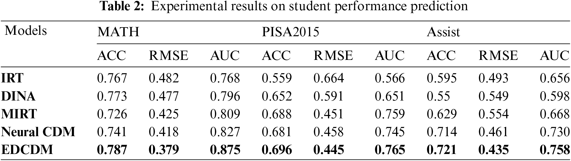
To evaluate whether the prediction performance of the model is generalizable across different datasets, we divided each dataset into an 80% training set and a 20% test set. The experimental results are shown in Table 2. The EDCD model outperformed almost all the baselines on both datasets, proving the effectiveness of the proposed model. For the MATH dataset, which contains both objective and subjective questions, the subjective part was discarded because the IRT, MIRT, and DINA models could not be applied to the subjective questions. For the PISA dataset, EDCDM also outperformed all baseline models in terms of prediction results. For the relatively sparse Assist dataset, the EDCDM model also produced the best experimental results overall. The interpretability of the traditional model was carried over to the EDCDM model, which also performed better overall than the neural CDM. The experiments showed that the traditional cognitive diagnostic model performed poorly on the sparse dataset.

The learning curve can also be utilized as a foundation for judgment to confirm that the suggested model has achieved convergence. To be more precise, 20% of the dataset is used as the test set, while the remaining 80% is used as the training set. We used three real-world datasets in our experiments, namely PISA 2015, mathematics, and auxiliary. During the training period, we record train loss, test loss and AUC metrics. Finally, EDCDM depicts the learning curve for each dataset, as shown in Fig. 3. The training loss, test loss, and AUC metric curves on all three datasets eventually level off, as shown in the learning curve plot above. Therefore, it can be assumed that given the relative number of current datasets, individual metrics can be made to converge and produce the desired training effect.

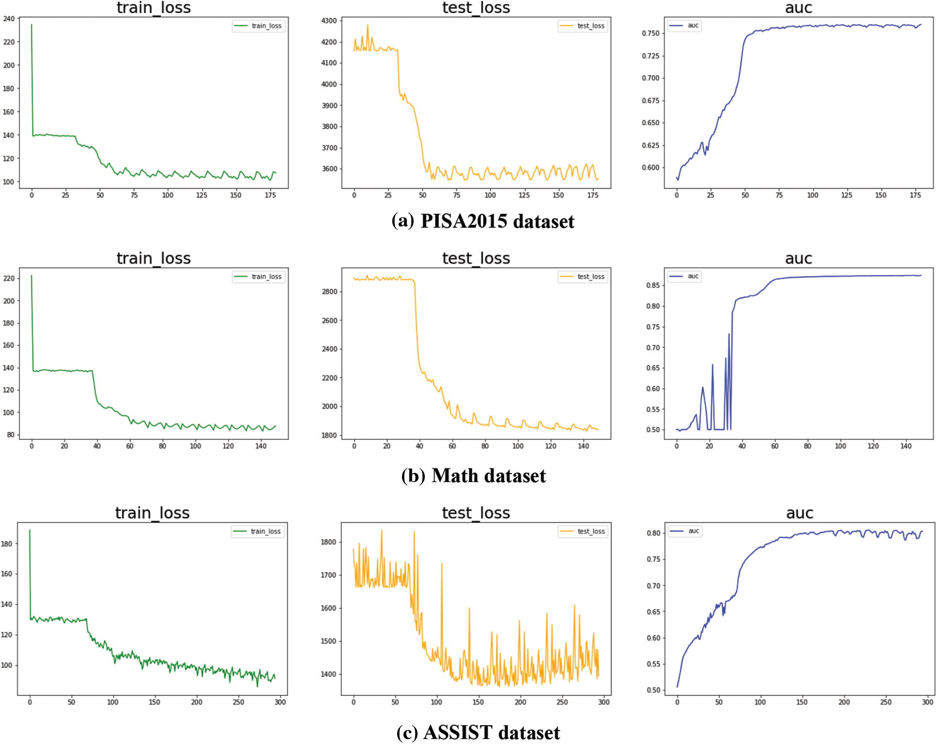
Figure 3: Convergence of EDCDM

4.3.2 Ablation Experiments

To verify the effect of each component in the proposed model on the accuracy of the EDCDM, we chose PISA and Math two datasets for the ablation experiments. We extended the EDCDM to verify the validity of the method used in the model with a 20% test rate. Table 3 gives the results of each index of the three extended experiments No_diff, No_skill, and No_gate on each dataset. No_diff is to disregard the difficulty of the test questions and set the difficulty parameter to 0; No_skill is to disregard the Q matrix, i.e., the skills tested by the test questions, similar to MIRT, which considers students to have multidimensional abilities; No_ gate is to disregard the factors of Slipping and Guessing, and to consider that students can answer the test questions correctly by mastering the skills tested by the test questions, without the mechanism of error tolerance.

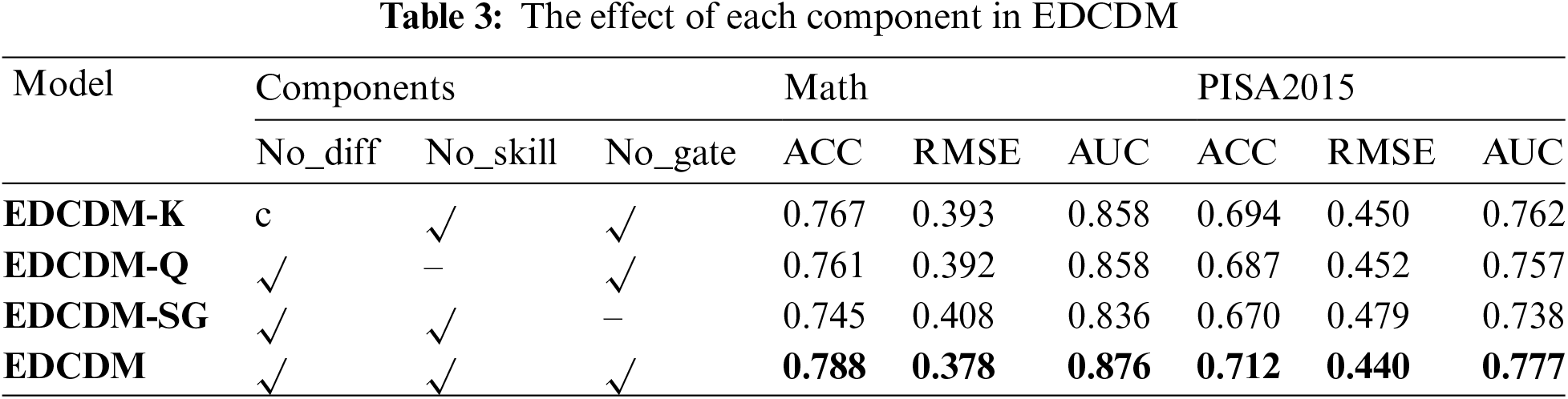
Compared to No_diff, the accuracy metric ACC metric improved by 0.019 on average and the error metric RMSE improved by 0.013 for EDCDM, indicating the validity of the difficulty representation of the test questions.

Compared to No_skill, the accuracy metric ACC metric improved by 0.026 on average and the error metric RMSE improved by 0.013 for EDCDM, indicating a positive effect of the skill interaction component on the prediction task.

Compared to No_diff, the accuracy metric ACC improved by 0.04 on average and the error metric RMSE improved by 0.03 for EDCDM, indicating that the screening gate mechanism (i.e., slipping and guessing factors) has an important role in the proposed model.

4.3.3 Monotonicity

To assess the monotonicity of the EDCDM (i.e., the higher the skill mastery, the higher the probability of answering the test questions correctly), we conducted experiments on different data sets. Fig. 4 shows the correlation between student’s skill mastery and response score, with three subplots representing the PISA, MATH, ASSIST datasets respectively.

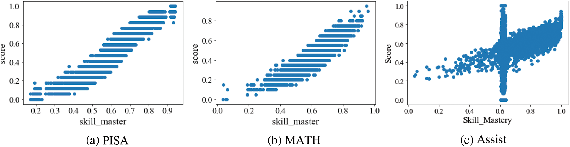
Figure 4: Monotonicity of EDCDM on three datasets

As can be seen from the figures, both subplots Figs. 4a and 4b perfectly fit the monotonicity assumption of the cognitive diagnostic theory. indicating that the proposed model performs well on the traditional dense data set. Fig. 4c is also consistent with the monotonicity assumption overall, however there are some outliers around a skill mastery level of 0.6. The students in these outliers have extremely few answer records, according to subsequent study. This finding shows that the monotonicity of the model needs to be further tuned on sparse dataset.

4.3.4 Case Study

We assessed the interpretability of the EDCDM by showing the distribution of students’ skill states through box plots and kernel density function plots. As shown in Fig. 5a for the neural CDM based on the mathematical dataset, the heat map of students’ mastery of all skills is almost the same color, indicating that there are almost no data fluctuations in their simulated values. In addition, the students’ mastery status for all attributes is mainly concentrated around 0.5 without any significant outliers. As shown in Fig. 5b, the EDCDM model based on the mathematical dataset has a more reasonable distribution of students’ mastery of all qualities, with balanced fluctuations, and has a more practical reference value.

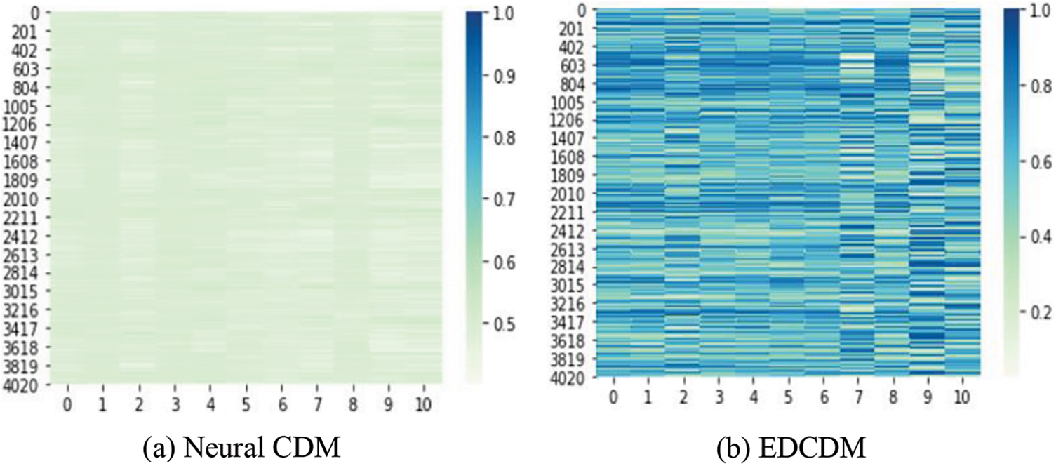
Figure 5: Visualization of skill states of Neural CD and EDCDM

Fig. 6 shows the distribution of EDCDM mastery for each skill in the PISA and MATH datasets respectively through box plots and kernel density distribution plots. Fig. 6a shows the distribution of mastery for each skill in the MATH dataset, with a median mastery of about 0.6 for each skill. Skill 2 is below average, indicating that it is more difficult. Skill 1 and Skill 3 were mastered at a much higher level than the others, indicating that they were less difficult. In addition, the distribution of students’ mastery of these two skills is spread out, suggesting that they can be used to more effectively differentiate students with different skills. Fig. 6b shows the distribution of mastery for each skill in the PISA dataset, with a median mastery of about 0.6 for each skill, and a median of about 0.7 for skill 4, indicating that this skill is relatively easy for students.

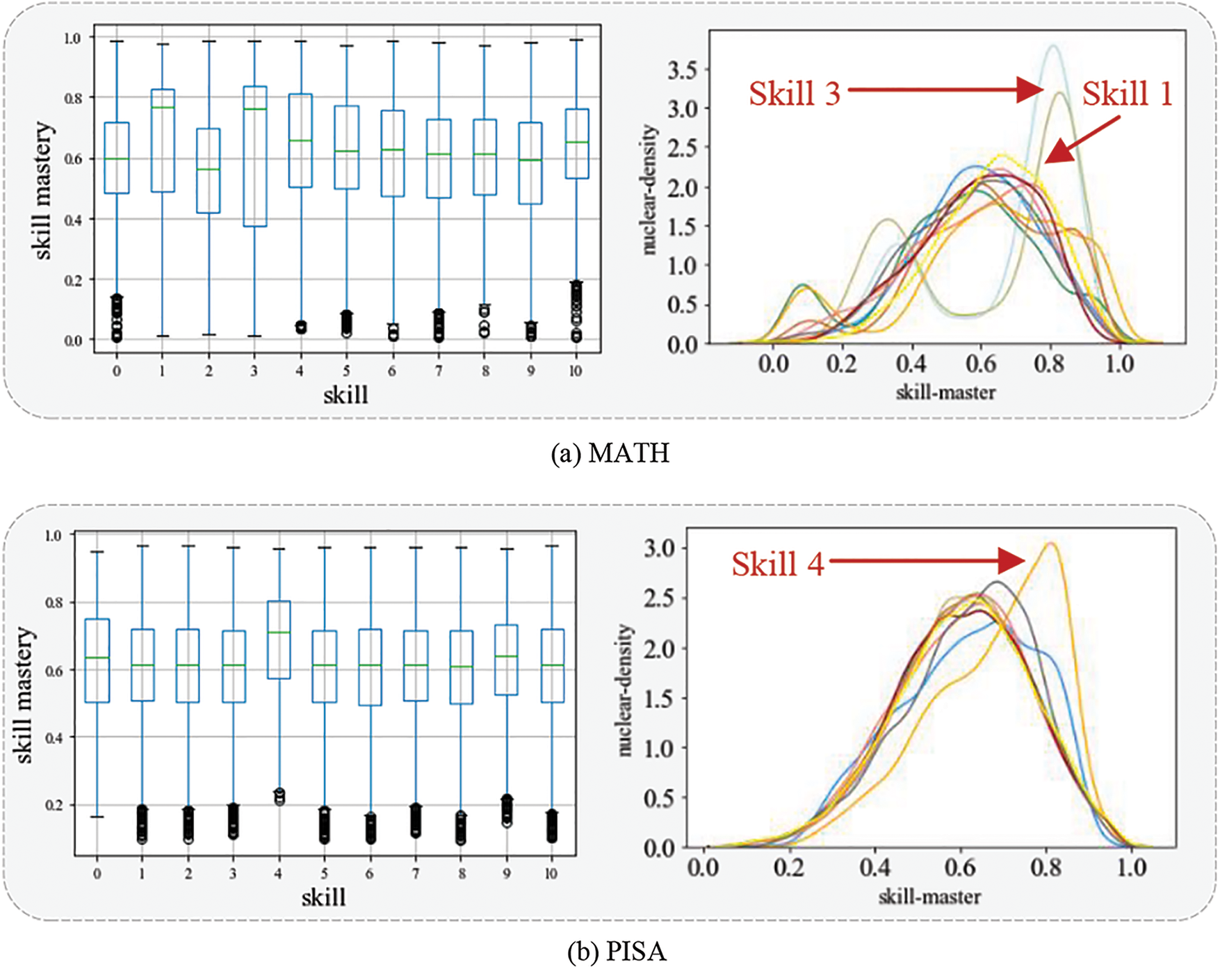
Figure 6: Distribution of mastery in each skill

5  Conclusion

To address the lack of modeling complex interactions between students and test questions in existing cognitive diagnostic models, this paper proposes a two-level augmented cognitive diagnostic model based on deep learning. EDCDM models students’ mastery of test questions through cognitive factors and then trains nonlinear interactions between students and test questions through neural networks to diagnose students’ skill mastery. By comparing with several baseline models, the following conclusions were obtained: (1) compared with other baseline models, EDCDM has higher accuracy in predicting student performance; (2) compared with other deep cognitive diagnostic models, EDCDM has good discrimination in diagnosing learners’ cognitive states, which makes the model have better explanatory power. With the continuous development and improvement of online learning, the research on cognitive diagnostic models and their applications for personalized learning will likely achieve technical breakthroughs in many aspects. Future work can be carried out in two aspects, namely dynamic cognitive modeling of students and cross-disciplinary knowledge transfer learning analysis, in order to realize the modeling of students’ cross-disciplinary cognitive states, which is important for a comprehensive understanding of students’ learning states and more accurate personalized learning tutoring.

Funding Statement: The authors received no specific funding for this study.

Availability of Data and Materials: The experimental data used to support the findings of this study are available from the corresponding author upon request.

Conflicts of Interest: The authors declare that they have no conflicts of interest to report regarding the present study.

1https://www.oecd.org/pisa/data/2015database/.

2https://sites.google.com/site/assistmentsdata/home/assistment-2009-2010-data/skill-builder-data-2009-2010.

References

1. R. F. F. Cima, B. Mazurek, H. Haider, D. Kikidis, A. Lapira et al., “A multidisciplinary European guideline for tinnitus: Diagnostics, assessment, and treatment,” HNO, vol. 67, no. 1, pp. 10–42, 2019. [Google Scholar] [PubMed]

2. M. Mohutsiwa and C. Musingwini, “Parametric estimation of capital costs for establishing a coal mine: South Africa case study,” Journal of the Southern African Institute of Mining and Metallurgy, vol. 115, no. 8, pp. 789–797, 2015. [Google Scholar]

3. Y. Cui, M. Gierl and Q. Guo, “Statistical classification for cognitive diagnostic assessment: An artificial neural network approach,” Educational Psychology, vol. 36, no. 6, pp. 1065–1082, 2016. [Google Scholar]

4. K. Wu, J. Liu, P. Liu and S. Yang, “Time series prediction using sparse autoencoder and high-order fuzzy cognitive maps,” IEEE transactions on fuzzy systems, vol. 28, no. 12, pp. 3110–3121, 2020. [Google Scholar]

5. A. M. Farhan, “Effect of rotation on the propagation of waves in hollow poroelastic circular cylinder with magnetic field,” Computers, Materials & Continua, vol. 53, no. 2, pp. 129–156, 2017. [Google Scholar]

6. X. Chen and J. H. Jiang, “A method of virtual machine placement for fault-tolerant cloud applications,” Intelligent Automation & Soft Computing, vol. 22, no. 4, pp. 587–597, 2016. [Google Scholar]

7. X. F. Li, Y. B. Zhuang and S. X. Yang, “Cloud computing for big data processing,” Intelligent Automation & Soft Computing, vol. 23, no. 4, pp. 545–546, 2017. [Google Scholar]

8. L. Ali, R. Sidek, I. Aris and M. A. M. Ali, “Design of a testchip for low cost IC testing,” Intelligent Automation & Soft Computing, vol. 15, no. 1, pp. 63–72, 2009. [Google Scholar]

9. J. Cheng, R. M. Xu, X. Y. Tang, V. S. Sheng and C. T. Cai, “An abnormal network flow feature sequence prediction approach for DDoS attacks detection in big data environment,” Computers, Materials & Continua, vol. 55, no. 1, pp. 95–119, 2018. [Google Scholar]

10. W. J. Yang, P. P. Dong, W. S. Tang, X. P. Lou, H. J. Zhou et al., “A MPTCP scheduler for web transfer,” Computers, Materials & Continua, vol. 57, no. 2, pp. 205–222, 2018. [Google Scholar]

11. Y. Chen, S. A. Culpepper, Y. Chen and J. Douglas, “Bayesian estimation of the DINA Q matrix,” Psychometrika, vol. 83, no. 1, pp. 89–108, 2018. [Google Scholar] [PubMed]

12. J. C. Zhou, D. H. Zhang, W. Q. Ren and W. S. Zhang, “Auto color correction of underwater images utilizing depth information,” IEEE Geoscience and Remote Sensing Letters, vol. 19, pp. 1–5, 2022. [Google Scholar]

13. C. Romero and S. Ventura, “Educational data mining: A review of the state of the art,” IEEE Transactions on Systems, Man, and Cybernetics, Part C (Applications and Reviews), vol. 40, no. 6, pp. 601–618, 2010. [Google Scholar]

14. J. de la Torre and J. A. Douglas, “Higher-order latent trait models for cognitive diagnosis,” Psychometrika, vol. 69, no. 3, pp. 333–353, 2004. [Google Scholar]

15. J. de la Torre, “DINA model and parameter estimation: A didactic,” Journal of Educational and Behavioral Statistics, vol. 34, no. 1, pp. 115–130, 2008. [Google Scholar]

16. J. de la Torre, “The generalized DINA model framework,” Psychometrika, vol. 76, no. 2, pp. 179–199, 2011. [Google Scholar]

17. M. von Davier, “The log-linear cognitive diagnostic model (LCDM) as a special case of the general diagnostic model (GDM),” ETS Research Report Series, vol. 2014, no. 2, pp. 1–13, 2014. [Google Scholar]

18. A. C. George and A. Robitzsch, “Validating theoretical assumptions about reading with cognitive diagnosis models,” International Journal of Testing, vol. 21, no. 2, pp. 105–129, 2021. [Google Scholar]

19. W. Song, L. Wen, L. Gao and X. Li, “Unsupervised fault diagnosis method based on iterative multi-manifold spectral clustering,” IET Collaborative Intelligent Manufacturing, vol. 1, no. 2, pp. 48–55, 2019. [Google Scholar]

20. M. Xi, “A study on the generalized cognitive diagnosis model of students based on BN network,” Modern Electric Electronic Technology, vol. 41, no. 24, pp. –79-81, 2018. [Google Scholar]

21. Y. Wang, “A cognitive diagnostic model of students’ psychological multilevel rating based on HO-DINA model research,” Modern Electric Electronic Technology, vol. 41, no. 2, pp. 53–55, 2018. [Google Scholar]

22. Q. Liu, R. Wu, E. Chen, G. Xu, Y. Su et al., “Fuzzy cognitive diagnosis for modelling examinee performance,” ACM Transactions on Intelligent Systems and Technology, vol. 9, no. 4, pp. 1–26, 2018. [Google Scholar]

23. R. T. Shan, Y. H. Luo and Y. Sun, “Collaborative filtering test recommendation based on cognitive diagnosis,” Computer System Applications, vol. 2018, no. 24, pp. 136–142, 2018. [Google Scholar]

24. T. E. Toprak and A. Cakir, “Examining the L2 reading comprehension ability of adult ELLs: Developing a diagnostic test within the cognitive diagnostic assessment framework,” Language Testing, vol. 38, no. 1, pp. 106–131, 2021. [Google Scholar]

25. P. Zhan, H. Jiao and D. Liao, “Cognitive diagnosis modelling incorporating item response times,” British Journal of Mathematical and Statistical Psychology, vol. 71, no. 21, pp. 262–286, 2018. [Google Scholar] [PubMed]

26. Z. Shu, R. Henson and J. Willse, “Using neural network analysis to define methods of DINA model estimation for small sample sizes,” Journal of Classification, vol. 30, no. 2, pp. 173–194, 2013. [Google Scholar]

27. K. K. Tatsuoka, “Rule space: An approach for dealing with misconceptions based on item response theory,” Journal of Educational Measurement, vol. 20, no. 4, pp. 345–354, 1983. [Google Scholar]

28. P. D. Zhan, H. Jiao, M. Q. Liao and Y. F. Bian, “Bayesian DINA modeling incorporating within-item characteristic dependency,” Applied Psychological Measurement, vol. 43, no. 2, pp. 143–158, 2019. [Google Scholar] [PubMed]

29. Y. Yang, Y. Zhang, L. Dai, J. Li, S. Mumtaz et al., “Transmission capacity analysis of relay-assisted device-to-device overlay/underlay communication,” IEEE Transactions on Industrial Informatics, vol. 13, no. 1, pp. 380–389, 2017. [Google Scholar]

References

1. L. Tetzlaff, F. Schmiedek and G. Brod, “Developing personalized education: A dynamic framework,” Educational Psychology Review, vol. 33, pp. 863–882, 2021. [Google Scholar]
2. A. Sun and X. Chen, “Online education and its effective practice: A research review,” Journal of Information Technology Education: Research, vol. 15, 2016. [Google Scholar]