A Comprehensive Evaluation of State-of-the-Art Deep Learning Models for Road Surface Type Classification

1  Introduction

The type of road surface is crucial information for intelligent transport systems (ITS), as it affects driver comfort and safety. For example, potholes or other damage, a sudden change to a more slippery surface, and other factors can make vehicle control difficult and lead to accidents. Classification of road surface types and their quality is essential for autonomous driving and advanced driver-assistance systems (ADAS) and road infrastructure departments for inspections. Regarding ADAS in self-driving navigation systems, surface type and quality classification can show how to drive more safely and comfortably. Regarding road infrastructure departments, the process of finding critical points can be sped up and made better if sections that need more attention and maintenance can be found automatically.

Accurate classification of a road surface is fundamental to improving vehicle dynamics. Numerous technologies, including anti-lock braking systems (ABS), traction control systems (TCS), connected vehicles (V2V), and vehicle-road infrastructure (V2I), can be fed with this information. Each to reach its full potential, the most exact surface properties are needed. With the development of these technologies, it will be possible to enhance performance, comfort, safety, and traffic management, among other things.

There are a variety of solutions proposed for this RST classification challenge. Based on a systematic literature review [1], RST classification can be divided into three main categories: three-dimensional (3D)-reconstruction-based, vision-based and sensor-based RST classification. The 3D reconstruction approaches rely on 3D laser scans to make accurate models of surfaces. Then, anomalies in the road surface are found by comparing these models to a baseline model. In this method, a 3D laser scanner uses reflected laser pulses to produce precise 3D digital representations of natural objects, including irregularities in the road’s surface. The distress features are then retrieved from the generated point clouds (i.e., a collection of points representing the three-dimensional form of road surface distress). This approach has been studied in detail by [2,3]. Nevertheless, the above methods necessitate expensive laser scanners [4] and are very expensive when keeping track of large road networks. Vision-based methods are based on the image processing analysis of captured images of damaged pavements. The fundamental idea behind this method is to make use of images that have been geotagged and were taken by a camera or video system that was installed on a moving vehicle with its downward-facing lens pointed toward the road surface. Using a method such as a Canny edge detection algorithm [5], it is possible to automatically detect any suspicious road surface distress features from the gathered geotagged video images, such as potholes and cracks. By [6,7], vision-based techniques were widely investigated. Even though these methods are less expensive than 3D reconstruction methods, they depend on ambient circumstances, such as lighting and shadow effects, among others [8]. In sensor-based techniques, road surface irregularities are recognized based on the vibration rate of driving cars, as measured by motion sensors (i.e., gyroscopes or accelerometers). Theoretically, when a vehicle goes over uneven road surfaces, such as potholes, cracks, manholes, or expansion joints, it is shaken more than it would be when driving over smooth road surfaces. The sensor-based approach is a viable, simple, low-cost solution [9]. Given these advantages of sensor technology, this work focuses on sensor-based RST classification.

Deep neural networks (DNNs) have recently progressed significantly in various sensor-based RST classification problems. A hierarchy of features, from low-level to high-level abstractions, can be automatically extracted and represent features to ones that have demonstrated their viability. DNNs circumvent the heuristic parameters of traditional hand-designed features and scale more effectively for more complicated behavior recognition tasks. Recent studies on deep learning (DL) methods have shown that DL methods are superior in classifying time series compared to hand-picked feature-based methods [10]. Convolutional Neural Networks (CNNs) is a DL technique frequently applied to sensor-based Human activity recognition (HAR). Even though sensor-based RST classification has been intensively researched, an effective feature-learning strategy must be exhaustively analyzed.

One downside to the DL paradigm, especially when using advanced DL architectures, is the increased cost of processing the vast datasets available. However, this cost is worth it because an RST classification system requires accurate results from the DL models.

In this study, researchers thoroughly analyze numerous state-of-the-art time-series classification models for RST using a CNN-based feature extractor that serves as the “backbone” of the formulation. Moreover, we developed an advanced DL model called SE-ResNet by embedding squeeze-and-excitation (SE) modules and residual connections to improve classification performances. Inspired by previous works, we take advantage of a residual network (ResNet) to extract more spatially abstract features of CNN. SE components were also integrated into the one-dimensional ResNet to enhance identification performance.

The critical contribution that makes our proposed technique outperform state-of-the-art techniques in the classification of RST can be summarized as follows:

•   A deep residual network (called SE-ResNet) is introduced for RST classification based on motion sensors (e.g., accelerometer, gyroscope, and magnetometer). The presented SE-ResNet works as a mixture of residual connections and channel attention mechanism of squeeze-and-excitation modules to improve classification performances.

•   We test our proposed model on a benchmark passive vehicular sensors (PVS) dataset that collected motion signals of vehicles while they were driven on three different road surface types. Experimental results show that our proposed SE-ResNet outperforms existing state-of-the-art models.

•   Based on experiments with different DL architectures, we found that the ResNet backbone is suitable for classifying RST using sensor data.

The rest of this study is broken into six sections: Section 2 reviews related works and the scientific background of RST classification. Section 3 describes the proposed methodology comprised of a sensor-based RST framework and a proposed deep residual model. Following that, Section 4 presents experimental studies using a benchmark dataset and compares the results of various DL models, including the proposed model. In Section 5, we examine the effect of sensor signals on the effectiveness of the RST classification system. Finally, Section 6 summarizes our results and possible future works.

2  Related Studies

This section summarizes previous research on RST classification based on sensor data. In addition, we provide brief reviews on state-of-the-art DL networks of time-series classification that are applicable for RST classification.

2.1 Sensor-Based Road Surface Type Classification

Few studies have been conducted during the past decade on the classification of road surface types using data from inertial sensors [11,12]. Two different vehicle types were used in the discovered experiments: ground robots on wheels [13,14] and cars [15–17]. Due to the significant structural differences between the two categories of vehicles and the fact that there is a dependence on the type of vehicle, we limited our review of the research to those that used sensors built into cars.

In [18,19], an accelerometer was attached to the suspension of the vehicle near the wheel on the right side of the vehicle. The acceleration and speed data collected by the global positioning system (GPS) were used to develop the machine learning (ML) models. The road was classified into four classes (asphalt, concrete, grass, and gravel) with an average accuracy of 69.4% using sensor data trained with a support vector machine.

The smartphone equipped with sensors was fastened to the area of the vehicle’s dashboard using a flexible suction mount, as described in [15]. The model used accelerometers and speed data from GPS. According to the study’s results, the model combining the complexity invariant distance and the longest common subsequence similarity yielded the best results. The road surface classification as asphalt/flexible pavement 98.28%, cobblestone streets 84.41%, and dirt roads 78.64% obtained an average accuracy of 87.68%.

After reviewing the related studies, we found that the studies use only acceleration and speed data, and ML models. These methods were limited by a feature extraction process that requires hand-crafted approaches to select appropriate features to construct efficient classification models.

2.2 State-of-the-Art DL Networks

In light of the importance of effectively classifying time series data, such as sensor data, we have proposed hundreds of learning-based algorithms as potential solutions to this problem [20]. This section examines the success of DL [21] on various classification problems, leading to the recent adoption of DL models for TSC [22]. The field of computer vision has changed radically with the introduction of deep CNNs [23]. As a result of the success of DNNs in computer vision, several DNN designs have been developed to address natural language processing (NLP) tasks such as word embedding learning, machine translation, and document classification. DNNs have also had a significant impact on the speech recognition community. Remarkably, the sequential nature of the data is the reason for the similarities between NLP and speech recognition tasks. Moreover, this is one of the essential characteristics of time series data [24].

Recently, we have gained attention for employing successful DL networks from the image domain to investigate their performance in the TSC domain. Fawaz et al. [25] developed an InceptionTime model based on the University of California–Riverside (UCR) time series archive to solve general TSC problems. They used the 85 datasets in the archive to compare and modify what the Hierarchical Vote Collective of Transformation-based Ensembles (HIVE-COTE) algorithm has been able to achieve with the same datasets. Ronald et al. [26] proposed the iSPLInception model, which builds on the Inception and ResNet backbones and employs a multichannel-residual composite architecture for sensor-based HAR research.

Analyzing related studies on DL approaches for TSC, we found that these models use CNN for automatic feature extraction. A CNN feature extractor is frequently referred to as the “backbone” when it comes to object identification. This is because the model architecture of the feature extractor and the overall model structure are evaluated in different ways. In this study, we comprehensively investigated other CNN backbone models and employed VGG16 [27], ResNet18 [28], PyramidNet18 [29], Inception-V3 [30], Xception [31], and EfficientNet B0. These models were proposed to solve the image recognition problem, so we rebuilt the architecture of the models for RST classification.

3  Proposed Methodology

In this section, we describe the process used to employ a DL model and classify road surface types using sensor data. The classification process is shown in Fig. 1. It comprises four stages: data acquisition, pre-processing, data generation, and training model and classification. Each step is described in detail below.

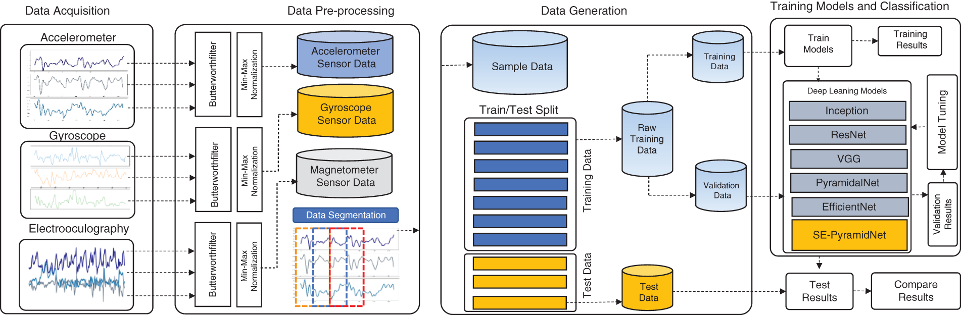
Figure 1: The methodology of RST classification based on sensor data

3.1 Data Acquisition

This study used a public benchmark called PVS dataset [32]. The vehicle was equipped with all sensors. The camera was mounted outside of the vehicle’s roof and set to record the environment at 30 Hz. The receiver GPS was installed internally within the dashboard and recorded data at 1 Hz. To accommodate data from points with different effects on the vehicle dependence attribute, six MPU-9250 modules were installed throughout the vehicle. Three MPU-9250s were placed at the right and left ends of the vehicle’s front axle: one module was placed on the vehicle’s handlebars, which were placed below and near the vehicle’s suspension; the second module was placed on the body directly above the tire and near the suspension; and a third module was placed on the vehicle’s dashboard in the passenger compartment. The controlled positioning method was applied to the MPU-9250 module’s sampling reference frame. The modules were placed so that the three axes of the sensor coordinate system were parallel to the vehicle’s axes.

Consequently, the vehicle became the reference frame for sampling and analysis. To prevent signal saturation, the accelerometer was calibrated to a full-scale value of 8 g, while the gyroscope was adjusted to 1,000 deg/s. Both instruments were recorded at 100 Hz. The PVS dataset was used to collect data from various contexts to obtain a variety of scenarios for the validation of the model. The previously described sensor network was utilized in three different vehicles, three different drivers with speeds ranging from 0 to 91.98 km/h, and three different scenarios in three other geographic locations, with each scenario having three different surface types, including unpaved and paved road sections. Details of the PVS dataset are shown in Table 1.

To fulfill the requirements of the PVS dataset, the inputs to the system consist of the sensor signals derived from the gyroscope, accelerometer, and magnetometer. To facilitate synchronization, all accelerometer, gyroscope, and magnetometer sensors on the MPU-9250 have been tuned to a sampling frequency of 100 Hz. Some raw sensor data recorded by the MPU-9250 are shown in Fig. 2.

Figure 2: Some raw sensor data collected in the PVS dataset

3.2 Pre-processing Process

Before proceeding with the analysis, it is necessary first to perform the data preprocessing step, which entails converting the raw data obtained from motion sensors into a clean and well-organized dataset. The raw data collected by the motion sensors typically contain measurement noise and other unanticipated noise. The signal noise obliterates relevant signal information. Therefore, it was critical to reduce the effects of noise on a motion to collect pertinent data for subsequent processing. The most commonly used filtering techniques are mean, low-pass, and Wavelet filtering. In our study, we applied a 3rd order low-pass Butterworth filter with a cutoff frequency of 20 Hz to the accelerometer and gyroscope sensors in all multiple dimensions to denoise the signals.

After analyzing each of the features evaluated, a separate normalization between [−1,1] was performed for each. Each chosen parameter’s various scales and units could have negatively impacted the model fit. This normalization minimized the above effect and ensured that the information for each variable was as representative as possible.

For data segmentation, the normalized data from all sensors are segmented into equally sized segments for further model training using a fixed-sized sliding window. In this study, a sliding window of two seconds with an overlapping proportion of 50% was used to generate sequences of sensor data with a length. Fig. 3 shows the data segmentation process used in this study.

Figure 3: The data segmentation process used in this work

3.3 The Proposed SE-ResNet

This work proposed a deep residual network called SE-ResNet, as shown in Fig. 4, to classify road surface types based on vehicle motion sensors efficiently. The architecture of the proposed SE-ResNet model consists of a global average-pooling layer, a fully connected layer, one convolution block, and eight residual blocks.

Figure 4: The architecture of the proposed SE-ResNet model

Numerous convolutional architectures are influenced by the discipline of image classification, where DL made its first and most significant advancements [33]. A highly effective method for dealing effectively with deeper networks is the utilization of what is known as skip connections, also known as residual connections. These connections traverse deeper neural networks while skipping numerous layers [34]. Furthermore, this neural network design has been modified for time series classification [35] and has shown comparably strong performance in various applications [36]. The number of residual modules is a hyperparameter of the ResNet architecture. An example of such a module is two convolutional layers and a jump link connecting the two layers (see Fig. 4).

CNNs are used to extract features by combining inputs in both spatial and channel-wise dimensions [37]. The representational power of a model can be increased by using a SE block, which was developed to factor in channel relationships. Fig. 5 shows the structure of the SE block. After the convolution operation, several feature maps are acquired. However, some feature maps may contain redundant information. The SE block performs feature recalibration to enhance the informative features and disable the less valuable ones. First, in the squeeze operation, global pooling is performed for each feature map, and a weight vector is determined. Then, in the excitation operation, fully connected layers and a sigmoid activation function are used to redistribute the feature weights. A gradient descent algorithm controls the redistribution. These weights are then used to reweight the feature maps. In this study, the SE block was moved behind the BN block in each residual block to recalibrate the feature maps generated from the stacked layers.

Figure 5: Structure of a squeeze-and-excitation module

3.4 Performance Evaluation

In the context of our studies, accuracy, and F1-score serve as evaluation criteria [38]. As we all know, most classification algorithms aim to minimize the overall error and maximize classification accuracy. However, for an imbalanced dataset, classification accuracy tells us relatively little about the minority class. Ironically, minority class members are often considered more exciting and vital. The classifier’s performance may be inaccurate and misleadingly evaluated if only accuracy is used to classify imbalanced classes. Therefore, we choose both accuracy and F1-score as evaluation measures to provide a more thorough evaluation of the classifier. The F1-score is an appropriate metric for evaluating classification performance for an imbalanced dataset. Since the F1-score shows how accuracy and recall affect each other, it shows whether a classifier achieves high recall by sacrificing accuracy or vice versa [39].

This study computed four evaluation metrics (accuracy, precision, recall, and F1-score) using a 5-fold cross-validation protocol to evaluate the performance of the proposed SE-ResNet model. The mathematical formula for these four performance criteria is as follows:

Accuracy=TP+TNTP+TN+FP+FN(1)

Precision=TPTP+FP(2)

Recall=TPTP+FN(3)

F1-score=2×Precision×RecallPrecision+Recall(4)

These four evaluation metrics are the most commonly used in RST classification to evaluate overall success. The recognition is characterized as true positive (TP) classification for the category under consideration and true negative (TN) identification for all other types evaluated. Passive vehicular sensor data from one class can also be misclassified as belonging to another category, resulting in a false positive (FP) classification for that category. Conversely, passive vehicular sensor data from another type can also be misclassified as belonging to that category, resulting in a false negative (FP) classification.

4  Experiments and Results

This section contains the results of all experimental studies conducted to determine the most efficient DL models for RST classification and the experiments’ results. Our experiments were performed using a benchmark dataset called PVS, which collected motion signals recorded while vehicles were driving on three different road surface types (dirt road, cobblestone road, and asphalt road). To evaluate the state-of-the-art models and our proposed SE-ResNet model, we conducted two experiments with 5-fold cross-validation. We used different sensor data from the dataset as follows:

•   Experiment I: we use motion signals from sensors located above and below the suspension on the left side of the vehicles.

•   Experiment II: we use motion signal data from sensors located above and below the suspension on the right side of the vehicles.

4.1 Environmental Configuration

The Google Collab Pro+ platform [40] was used for the experiments. The results of accelerating the training of DL models using the Tesla V100-SXM2 with a 16 GB graphics processor (GPU) module were impressive. The Python library was used to implement the proposed SE-ResNet and advanced DL models using the Tensorflow backend (version 3.9.1) [41] and CUDA (version 8.0.6) [42] graphics cards. This study focused on the following Python libraries, which are listed below:

•   The sensor data was processed using Numpy and Pandas, which comprised reading, processing, and analyzing the data.

•   The results of the data acquisition and model evaluation procedures were plotted and displayed using Matplotlib and Seaborn.

•   Sklearn is a library used in research as a sampling and data generation tool.

•   TensorFlow, Keras, and TensorBoard were used to develop and train the DL models, among others.

4.2 Hyperparameter Setting

Hyperparameter values are used to regulate the learning process in DL. The following hyperparameters are used in the proposed SE-ResNet model: (i) the number of epochs, (ii) the batch size, (iii) the learning rate α, (iv) the optimization and (v) the loss function. The values of these hyperparameters were determined by setting the number of epochs to 200 and the batch size to 128. If there was no improvement in the validation loss after 20 epochs, the training process was terminated by an early-stop callback. The initial conditions for the learning rate are α = 0.001. If the validation accuracy of the proposed model had not improved after six consecutive epochs, we changed it to 75% of the previous value. To minimize the error, we used the Adam optimizer [43] with parameters β1 = 0.9, β2 = 0.999, and ε = 1×10−8. The categorical cross-entropy function is used to determine the optimizer’s error. Recently, the cross-entropy technique was outperformed other methods (i.e., classification and mean square errors) [44]. We set the weights in the SE-ResNet to prepare the model using Xavier initialization. Then we iteratively trained the model for 200 epochs.

4.3 Experimental Results of Experiment I

The results of Experiment I used an accelerometer, gyroscope, and magnetometer, and data was recorded from three MPU-9250s placed on the left side of the vehicles. The results of the SE-ResNet and state-of-the-art models are summarized in Table 2.

From the comparative results in Table 2, it can be seen that our proposed SE-ResNet model outperformed the other DL models in this experiment with the highest accuracy of 98.37% and the highest F1-score of 98.15%. Comparing the backbone architecture of the state-of-the-art models, we observe that the ResNet backbone has higher accuracy than other models. This is because ResNets use the residual structure while strengthening the feature at each convolution stage.

Fig. 6 shows the process of learning raw sensor data from the left side of vehicles with the proposed SE-ResNet. With the epoch at 50, the loss rate decreased significantly, and the accuracy stabilized significantly. Finally, the accuracy was 98.37% in the testing set. After that, the loss rate decreased gradually, and the accuracy rate increased slowly without any appearance of dilemma. This indicates that the network learns appropriately without overfitting problems.

Figure 6: Accuracy and loss rate of the training process of the proposed SE-ResNet from experiment I

4.4 Experimental Results of Experiment II

The results from Table 3 indicate that our SE-ResNet model achieved the best results in this experiment. The proposed model achieved the highest accuracy of 98.41% and the highest F1-score of 98.19% in this experiment which outperforms other state-of-the-art models.

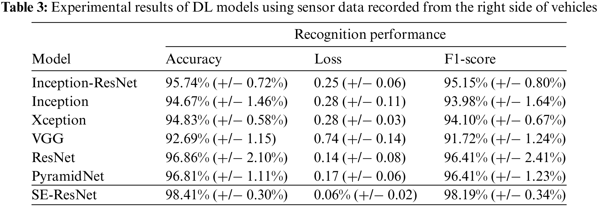
Fig. 7 shows a satisfactory learning process of learning raw sensor data from the right side of vehicles with the proposed SE-ResNet. The accuracy quickly stabilized, which achieved 98.41% in the testing set. The loss rate decreased gradually, and the accuracy rate increased slowly without any appearance of dilemma. This indicates that the network learns appropriately without overfitting problems.

Figure 7: Accuracy and loss rate of the training process of the proposed SE-ResNet from experiment II

5  Discussion

5.1 Effects of Placement

To illustrate the impact of the MPU-9250 modules on the performance of the proposed SE-ResNet model, the comparative results are shown in Table 4. These results indicate that the model has good learning and generalization capabilities in all placement experiments.

To discover details of the classification performance, we examine the confusion matrices for all, as shown in Fig. 8. These results show that the different placements do not affect the RST classification.

Figure 8: Comparison of the model performance between confusion matrices: (a) results of the Experiment I (b) results of experiment II

5.2 Effects of Squeeze-and-Excitation Mechanism

For most learning-based applications, the capacity to learn an interpretable representation is essential. The advantage of DL approaches is that they can extract features from raw data. Still, it can be challenging to understand how much each input dataset contributed relative to the others. Previous research [37] has developed the concept of a squeeze-and-excitation mechanism to overcome this problem. In this investigation, a SE mechanism designed for neural networks for machine translation tasks was integrated into our classification system. This work assisted in creating an understandable representation that highlights the most critical points of each input data segment of the model. The results showed that the SE mechanism improved the classification performance in each case, as shown in Tables 5 and 6. In particular, our SE-ResNet model showed significantly better performance in Experiments I and II.

5.3 Comparative Analysis

A comparison between the proposed RE-ResNet and other DL networks (CNN, LSTM, and CNN-LSTM) studied in previous works is shown in Table 7. The SE-ResNet network outperformed the other networks. This is because the spatial feature extraction performed by the SE-ResNet improved the overall performance.

6  Conclusion and Future Works

In this work, we implemented state-of-the-art DL models for sensor-based RST classification. The models aimed to classify three different road types. We also developed a DL called SE-ResNet to improve the classification performance. The proposed SE-ResNet is a new DL model that combines the benefits of connection modules with squeeze-and-excitation modules to improve RST classification accuracy. The performance of all DL models was evaluated against a publicly available benchmark dataset called PVS. The dataset collected large numbers of motion data from sensors placed at different positions of vehicles. The conducted experiments and comparative analysis show that the proposed SE-PyramidNet outperforms the other state-of-the-art models. The SE-ResNet achieved the highest accuracy of 98.41% and the F1-score of 98.19%. Moreover, the proposed RE-ResNet outperformed the other DL networks (CNN, LSTM, and CNN-LSTM). The proposed RE-ResNet achieved the classification accuracies of asphalt roads at 98.98, cobblestone roads at 97.02, and dirt roads at 99.56%, respectively.

We extensively analyzed the experimental results and found that the PyramidNet backbone is suitable for RST classification. In addition, we developed the SE-ResNet, which is based on a ResNet backbone and squeeze-and-excitation modules. Our results show that channel attention can improve RST classification performances. As a module in autonomous vehicles, the proposed SE-ResNet can classify RST and adapt the driving mode to such situations. Situational data can support various applications. Since the surface type affects fuel consumption, travel duration, and vehicle damage, production flow and logistics systems can use this data to develop cost-effective routes.

In the future, we will work to overcome one of the drawbacks of the original study: the requirement for sensor data with a predetermined size with adaptive data segmentation. In addition, we intend to develop a hierarchical learning approach to improve RST classification.

Funding Statement: This project is funded by National Research Council of Thailand (NRCT): An Integrated Road Safety Innovations of Pedestrian Crossing for Mortality and Injuries Reduction Among All Groups of Road Users, Contract No. N33A650757. This project was also supported by the Thailand Science Research and Innovation Fund; the University of Phayao (Grant No. FF66-UoE001); King Mongkut’s University of Technology North Bangkok under Contract No. KMUTNB-66-KNOW-05.

Conflicts of Interest: The authors declare that they have no conflicts of interest to report regarding the present study.

References

1. S. Sattar, S. Li and M. Chapman, “Road surface monitoring using smartphone sensors: A review,” Sensors, vol. 18, no. 11, pp. 3845, 2018. [Google Scholar] [PubMed]

2. H. W. Wang, C. H. Chen, D. Y. Cheng, C. H. Lin and C. C. Lo, “A real-time pothole detection approach for intelligent transportation system,” Mathematical Problems in Engineering, vol. 2015, no. 869627, pp. 1–7, 2015. [Google Scholar]

3. W. Y. Yan, A. Shaker and N. El-Ashmawy, “Urban land cover classification using airborne LiDAR data: A review,” Remote Sensing of Environment, vol. 158, pp. 295–310, 2015. [Google Scholar]

4. T. Kim and S. Ryu, “Review and analysis of pothole detection methods,” Journal of Emerging Trends in Computing and Information Sciences, vol. 5, pp. 603–608, 2014. [Google Scholar]

5. J. Canny, “A computational approach to edge detection,” IEEE Transactions on Pattern Analysis and Machine Intelligence, vol. 8, no. 6, pp. 679–698, 1986. [Google Scholar] [PubMed]

6. W. Y. Yan and X. X. Yuan, “A low-cost video-based pavement distress screening system for low-volume roads,” Journal of Intelligent Transportation Systems, vol. 22, no. 5, pp. 376–389, 2018. [Google Scholar]

7. L. Huidrom, L. K. Das and S. Sud, “Method for automated assessment of potholes, cracks and patches from road surface video clips,” Procedia Social and Behavioral Sciences, vol. 104, pp. 312–321, 2013. [Google Scholar]

8. Y. Wu, H. Guo, C. Chakraborty, M. Khosravi, S. Berretti et al., “Edge computing driven low-light image dynamic enhancement for object detection,” IEEE Transactions on Network Science and Engineering, vol. 1, pp. 1, 2022. [Google Scholar]

9. I. S. Andrades, J. J. Castillo Aguilar, J. M. V. García, J. A. C. Carrillo and M. S. Lozano, “Low-cost road-surface classification system based on self-organizing maps,” Sensors, vol. 20, no. 21, pp. 6009, 2020. [Google Scholar] [PubMed]

10. S. Usmankhujaev, B. Ibrokhimov, S. Baydadaev and J. Kwon, “Time series classification with inception FCN,” Sensors, vol. 22, no. 1, pp. 157, 2022. [Google Scholar]

11. J. Menegazzo and A. Von Wangenheim, “Vehicular perception and proprioception based on inertial sensing: A systematic review,” Federal University of Santa Catarina-Brazilian National Institute for Digital Convergence-Technical Reports, 2018. [Google Scholar]

12. J. Menegazzo and A. Von Wangenheim, “Vehicular perception based on inertial sensing: A structured mapping of approaches and methods,” SN Computer Science, vol. 1, no. 5, pp. 1–24, 2020. [Google Scholar]

13. S. Khaleghian and S. Taheri, “Terrain classification using intelligent tire,” Journal of Terramechanics, vol. 71, no. 4, pp. 15–24, 2017. [Google Scholar]

14. B. Sebastian and P. Ben-Tzvi, “Support vector machine based real-time terrain estimation for tracked robots,” Mechatronics, vol. 62, no. 2, pp. 102260, 2019. [Google Scholar]

15. V. M. Souza, “Asphalt pavement classification using smartphone accelerometer and complexity invariant distance,” Engineering Applications of Artificial Intelligence, vol. 74, no. 3, pp. 198–211, 2018. [Google Scholar]

16. S. Wang, S. Kodagoda, L. Shi and X. Dai, “Two-stage road terrain identification approach for land vehicles using feature-based and markov random field algorithm,” IEEE Intelligent Systems, vol. 33, no. 1, pp. 29–39, 2018. [Google Scholar]

17. S. Wang, S. Kodagoda, L. Shi and H. Wang, “Road-terrain classification for land vehicles: Employing an acceleration-based approach,” IEEE Vehicular Technology Magazine, vol. 12, no. 3, pp. 34–41, 2017. [Google Scholar]

18. S. Wang, S. Kodagoda, L. Shi and X. Dai, “Two-stage road terrain identification approach for land vehicles using feature-based and markov random field algorithm,” IEEE Intelligent Systems, vol. 33, no. 1, pp. 29–39, 2018. [Google Scholar]

19. S. Wang, S. Kodagoda, L. Shi and H. Wang, “Road-terrain classification for land vehicles: Employing an acceleration-based approach,” IEEE Vehicular Technology Magazine, vol. 12, no. 3, pp. 34–41, 2017. [Google Scholar]

20. A. Bagnall, J. Lines, A. Bostrom, J. Large and E. Keogh, “The great time series classification bake off: A review and experimental evaluation of recent algorithmic advances,” Data Mining and Knowledge Discovery, vol. 31, no. 3, pp. 606–660, 2017. [Google Scholar] [PubMed]

21. Y. LeCun, Y. Bengio and G. Hinton, “Deep learning,” Nature, vol. 521, no. 7553, pp. 436–444, 2015. [Google Scholar] [PubMed]

22. Z. Wang, W. Yan and T. Oates, “Time series classification from scratch with deep neural networks: A strong baseline,” in 2017 Int. Joint Conf. on Neural Networks (IJCNN), Anchorage, Alaska, USA, pp. 1578–1585, 2017. [Google Scholar]

23. A. Krizhevsky, I. Sutskever and G. E. Hinton, “ImageNet classification with deep convolutional neural networks,” in Advances in Neural Information Processing Systems 25: 26th Annual Conf. on Neural Information Processing Systems 2012 (NIPS 2012), Lake Tahoe, Nevada, United States, pp. 1097–1105, 2012. [Google Scholar]

24. H. Ismail Fawaz, G. Forestier, J. Weber, I. Lhassane and M. Pierre-Alain, “Deep learning for time series classification: A review,” Data Mining and Knowledge Discovery, vol. 33, no. 4, pp. 917–963, 2019. [Google Scholar]

25. H. I. Fawaz, B. Lucas, G. Forestier, C. Pelletier, D. F. Schmidt et al., “InceptionTime: Finding AlexNet for time series classification,” Data Mining and Knowledge Discovery, vol. 34, no. 6, pp. 1936–1962, 2020. [Google Scholar]

26. M. Ronald, A. Poulose and D. S. Han, “iSPLInception: An inception-ResNet deep learning architecture for human activity recognition,” IEEE Access, vol. 9, pp. 68985–69001, 2021. [Google Scholar]

27. K. Simonyan and A. Zisserman, “Very deep convolutional networks for large-scale image recognition,” eprint arXiv:1409.1556, vol. 1, 2014. [Google Scholar]

28. K. He, X. Zhang, S. Ren and J. Sun, “Deep residual learning for image recognition,” in 2016 IEEE Conf. on Computer Vision and Pattern Recognition (CVPR), Las Vegas, NV, USA, pp. 770–778, 2016. [Google Scholar]

29. D. Han, J. Kim and J. Kim, “Deep pyramidal residual networks,” in 2017 IEEE Conf. on Computer Vision and Pattern Recognition (CVPR), Honolulu, HI, USA, pp. 5927–5935, 2017. [Google Scholar]

30. C. Szegedy, V. Vanhoucke, S. Ioffe, J. Shlens, Z. Wojna et al., “Rethinking the inception architecture for computer vision,” in 2016 IEEE Conf. on Computer Vision and Pattern Recognition (CVPR), Las Vegas, NV, USA, pp. 2818–2826, 2016. [Google Scholar]

31. F. Chollet, “Xception: Deep learning with depthwise separable convolutions,” in 2017 IEEE Conf. on Computer Vision and Pattern Recognition (CVPR), Honolulu, HI, USA, pp. 1251–1258, 2017. [Google Scholar]

32. T. Lee, C. Chun and S. -K. Ryu, “Detection of road-surface anomalies using a smartphone camera and accelerometer,” Sensors, vol. 21, no. 2, pp. 561, 2021. [Google Scholar] [PubMed]

33. N. Zaman, L. Gaur and M. Humayun, “Approaches and applications of deep learning in virtual medical care,” in IGI Global, pp. 127–167, 2022. [Online]. Available: https://ouci.dntb.gov.ua/en/works/40DxOjy4/. [Google Scholar]

34. K. He, X. Zhang, S. Ren and J. Sun, “Deep residual learning for image recognition,” in 2016 IEEE Conf. on Computer Vision and Pattern Recognition (CVPR), Las Vegas, NV, USA, pp. 770–778, 2016. [Google Scholar]

35. Z. Wang, W. Yan and T. Oates, “Time series classification from scratch with deep neural networks: A strong baseline,” in 2017 Int. Joint Conf. on Neural Networks (IJCNN), Anchorage, Alaska, USA, pp. 1578–1585, 2017. [Google Scholar]

36. H. Ismail Fawaz, G. Forestier, J. Weber, L. Idoumghar and P. -A. Muller, “Deep learning for time series classification: A review,” Data Mining and Knowledge Discovery, vol. 33, no. 4, pp. 917–963, 2019. [Google Scholar]

37. A. Muqeet, M. T. B. Iqbal and S. H. Bae, “HRAN: Hybrid residual attention network for single image super-resolution,” IEEE Access, vol. 7, pp. 137020–137029, 2019. [Google Scholar]

38. A. Ali, S. M. Shamsuddin and A. L. Ralescu, “Classification with class imbalance problem: A review,” International Journal of Advances in Soft Computing and its Applications, vol. 7, no. 3, pp. 176–204, 2015. [Google Scholar]

39. S. S. Kshatri, K. Thakur, M. H. Mamode Khan, D. Singh and G. R. Sinha, “Computational intelligence and applications for pandemics and healthcare,” in IGI Global, pp. 83–113, 2022. [Online]. Available: https://www.researchgate.net/publication/360034430_Machine_Learning. [Google Scholar]

40. E. Bisong, “Building machine learning and deep learning models on Google cloud platform: A comprehensive guide for beginners,” in Apress, 2019. [Online]. Available: https://link.springer.com/book/10.1007/978-1-4842-4470-8. [Google Scholar]

41. M. Abadi, P. Barham, J. Chen, Z. Chen, A. Davis et al., “Tensorflow: A system for large-scale machine learning,” in 12th USENIX Symp. on Operating Systems Design and Implementation (OSDI ‘16), Savannah, GA, USA, pp. 265–283, 2016. [Google Scholar]

42. NVIDIA Corporation, “Introduction to NVIDIA GPU cloud,” NVIDIA Corporation Application Note, 2022. [Online]. Available: https://www.nvidia.com/en-us/data-center/gpu-cloud-computing/. [Google Scholar]

43. D. P. Kingma and J. Ba, “Adam: A method for stochastic optimization,” in Int. Conf. on Learning Representations (ICLR), Banff, Canada, 2014. [Google Scholar]

44. K. Janocha and W. M. Czarnecki, “On loss functions for deep neural networks in classification,” Schedae Informaticae, vol. 25, pp. 49–59, 2016. [Google Scholar]

45. J. Menegazzo and A. V. Wangenheim, “Road surface type classification based on inertial sensors and machine learning,” Computing, vol. 103, no. 10, pp. 2143–2170, 2021. [Google Scholar]