Anomaly Detection for Cloud Systems with Dynamic Spatiotemporal Learning

1  Introduction

Currently, cloud systems with large-scale distributed architectures are becoming more complex [1]. Meanwhile, the workload of information technology (IT) operations is growing dramatically [2]. System administrators are experiencing various unexpected failures [3]. In addition, unlike most legacy software, whose failures can be reported directly through error messages or some other observable anomaly indications, modern cloud systems often run out of order imperceptibly [4]. The reasons for this phenomenon are as follows. Cloud services are usually supported by large-sized clusters with high complexity. Thus, cloud systems rarely break down by throwing explicit exception messages or interrupted processes. Instead, such systems with anomalies tend to perform as “partially available, partially unavailable” or “most of the functions are available, but a few are not.” We call this phenomenon “weakly available.” That may induce a hardship in which the operations and maintenance staff react passively only after their customers’ business has been severely impacted. It is nontrivial but valuable to proactively detect subtle anomalies that lurk in complex cloud systems.

Although many research efforts have been devoted to solving the problem of detecting system anomalies in recent years, most have focused on the system’s individual metrics or key performance indicators (KPIs), such as in references [5,6]. However, as the cloud system complexity increases, it becomes increasingly difficult to train and maintain respective models for every component. Especially for systems composed of microservices, the number of KPIs grows exponentially, bringing numerous monitoring demands. Moreover, when determining whether a module is anomalous, the metrics or KPIs to review should not be confined to that component but include others in correlation with it. The demands above challenge general machine learning models. It concerns that, for large-scale cloud systems, ignoring the interactions among submodules will likely lose insights into their internal topology and may eventually lead to limitations on the anomaly detection models.

1.1 Research Motivation

We explain the hardship of anomaly detection for complex systems with an example of contrast analysis. The case is from an elasticsearch cluster. Elasticsearch is a distributed search engine popular in the industry [7]. In our example, the elasticsearch cluster is composed of five peer-to-peer nodes. We set up two groups of writers writing to the elasticsearch with homogeneous contents but different writing modes. Then, we compare the performance of the two groups.

First, we give the runtime monitoring of Group 1. There are five parallel clients in Group 1, each of which writes to its corresponding index as one-to-one mapping without crossover, and they write at nearly the same rate. The monitoring of the servers and clients in Group 1 during parallel writing is displayed in Fig. 1.

Figure 1: Monitoring of Group 1

Then, we give the runtime monitoring of Group 2. Similar to Group 1, Group 2 also has five parallel clients. The writing rate and content from each client in Group 2 were consistent with those in Group 1. However, the difference from Group 1 is that the clients in Group 2 did not have a one-to-one mapping with the indices. In Group 2, three clients shared writing indices with each other. The data distribution among cluster nodes is skewed, as most data are submitted to the same index. The monitoring of the servers and clients in Group 2 during parallel writing is displayed in Fig. 2.

Figure 2: Monitoring of Group 2

From the monitoring results in Figs. 1 and 2, the differences in performance between Group 1 and Group 2 are mainly on the client side. In Group 1, the write rate of each client is high and consistent (above 2,000,000), while in Group 2, the write rate of Clients 1–3 fluctuates significantly, with clear lows (below 2,000,000) from time to time. Broadly speaking, in Group 2, the monitoring of memory and CPU indicators shows no abnormal fluctuations (the metrics of Node 4 are slightly higher on average, but they are still within the normal range). No particular abnormalities were observed on the severe side of either Group 1 or Group 2. However, as indicated by the red marks in Fig. 2, a closer look at the monitoring of Group 2 shows that the metrics of resource usage on Node 1, Node 3, and Node 4 almost overlap at peak when there are slight delays in Client 1, Client 2, and Client 3, respectively. Meanwhile, the metrics in Group 2 display a relatively larger amplitude of oscillation than in Group 1. This phenomenon occurs because Clients 1–3 cross-wrote to the same indices, and the affected skewed indices are managed by Node 1, Node 3, and Node 4.

In this example, the clients of Group 2 may have sensed something is not in harmony, but at the same time, it is hard to detect the subtle anomalies from individual monitoring on the server side. For this case, when deciding whether a service is in health, it is necessary to consider the various components connected and the interactions between them, not just the properties of the individual service.

1.2 Contributions

Aiming at the problem of anomaly detection in complex cloud systems, this paper makes the following contributions. We propose an anomaly detection method for cloud systems with dynamic spatiotemporal learning. For convenience, it is abbreviated as AD-DSTL. AD-DSTL models the collaborative cluster as a graph. The graph model represents the system topology, in which the service endpoints or process instances are regarded as nodes, and the interactions between them are regarded as connections. AD-DSTL not only deliberates on the temporal dynamics of various properties on both nodes and connections but also considers spatial dynamics such as connection generation and disconnection. The core implementation of AD-DSTL is an end-to-end spatial-temporal deep learning network. We conduct experiments on four datasets. The results show that AD-DSTL outperforms other alternative methods in terms of overall performance. In addition to the comparative evaluation, ablation studies are carried out from multiple perspectives to sufficiently validate the effect of various factors on AD-DSTL. We have released partial source code and one new dataset publicly [8], allowing for easy use by researchers and practitioners for future studies.

The remainder of this paper is organized as follows. Section 2 examines the related work. Section 3 sets up several essential concepts and defines the objective problem. Section 4 depicts the details of AD-DSTL. Section 5 presents the experimental analysis. Section 6 concludes this paper.

2  Related Work

Many works have studied anomaly detection from various levels and perspectives. In the context of this paper, related research can be divided into two categories: common detection algorithm research and detection method research targets for cloud service maintenance scenarios. The first category focuses on the development of basic anomaly detection algorithms, while the second category centers on creating specialized techniques for detecting anomalies in cloud service maintenance scenarios. Next, we will explore the relevant literature according to the above categories.

2.1 Generic Anomaly Detection Algorithms

The demands of anomaly detection exist in various fields, such as disease detection, financial fraud detection, and network intrusion detection. Therefore, anomaly detection is usually abstracted as a science research question. Some work has been carried out based on knowledge and rules [9]. Nevertheless, as far as research development is concerned, more researchers have chosen data-driven techniques, which detect anomalies based on data reflecting the target’s state [10].

Most of the earlier data-driven methods leverage statistical techniques, assuming that the data obey some distribution and estimate the parameters of the probabilistic model. The advantage of statistical methods is that they are suitable for low-dimensional data and have better robustness. However, these methods rely heavily on distribution assumptions and are less able to adapt to dynamic changes in data distribution. Many research efforts, such as literature [11], have developed clustering-based anomaly detection algorithms. The disadvantage of the clustering approach is that it usually just gives a 0/1 result (i.e., whether it is an anomaly or not) but cannot quantify the degree of an anomaly for each data point. In addition, the performance of the clustering-based techniques depends heavily on whether the clustering algorithm can capture the clustering structure of normal instances. The local outlier factor (LOF) is another well-known method for anomaly detection [12]. It is a classical density-based algorithm that can quantify the degree of an anomaly for outliers and does not depend on the data distribution.

With the development of deep learning in recent years, many anomaly detection models based on deep learning techniques have emerged [13,14]. Deep learning-based models have gained much attention in recent years because they are better at modeling complex dependencies in data. For example, Ergen et al. [15] investigated anomaly detection in an unsupervised framework and introduced long short-term memory (LSTM) neural network-based algorithms. Ding et al. [16] studied the anomaly detection problem on attributed networks by developing a novel deep model; it used a graph convolutional network (GCN) to synthesize the structure information of the graph to obtain the embedding of nodes and then leveraged the learned embeddings to reconstruct the original data by using an autoencoder. Pang et al. [17] surveyed the research of deep learning-enabled anomaly detection and showed the importance of deep anomaly detection.

The above research on generic anomaly detection problems provides a basic reference for system operation and maintenance detection. However, to achieve the best practical results, it is usually necessary to further combine the characteristics of the problems in the system operation and maintenance and design methods that are closer to realistic needs, more feasible, and more effective in application. In this paper, a system anomaly detection method based on spatiotemporal deep learning is designed precisely close to realistic system operation and maintenance problems.

2.2 Anomaly Detection Methods for System Operation and Maintenance

The detection of anomalies in running IT systems is a critical concern for system maintenance, and much research has been conducted specifically in this area. Unlike ordinary studies on generic algorithms, research in this area usually needs to take advantage of actual business characteristics and then flexibly apply suitable anomaly detection algorithms. For example, Wang et al. [18] proposed a progressive exploration framework for collective anomaly detection on network traffic based on a clustering method. This framework enables analysts to effectively explore collective anomalies in network traffic. Islam et al. [19] designed a deep learning-based anomaly detector for system logs. This system utilized deep learning neural networks to detect anomalies in near real-time in multiple platform components simultaneously. Du et al. [20] designed a deep learning-based anomaly detector for system logs. Soldani et al. [21] provided a structured overview and qualitative analysis of currently available techniques for anomaly detection and root cause analysis in modern multiservice applications.

In recent years, some literature on system anomaly detection has involved constructing a graph-based representation for the system [22–24]. In particular, He et al. [24] focused on capturing the spatiotemporal characteristics of cloud systems and created a deep learning model for anomaly detection using a graph neural network (GNN) and a recurrent neural network (RNN). However, that work has several limitations regarding the spatial modeling of the system topology. First, it does not account for the dynamics of the system topology over time. Second, it only considers the node elements but not the connections of the system topology. In addition, it obtains the final anomaly score on the nodes. However, the anomaly of complex systems is usually systematic. This paper focuses on bridging these gaps and designing a more easily implemented spatiotemporal deep learning network. Moreover, unlike in the above research study, this paper takes into account that modern system operations and maintenance will be supported by sophisticated automated platforms that can provide sufficient data for supervised training of deep learning models. Therefore, the model designed in this paper adopts a supervised model that is easier to implement and more effective in practice.

3  Problem Statement

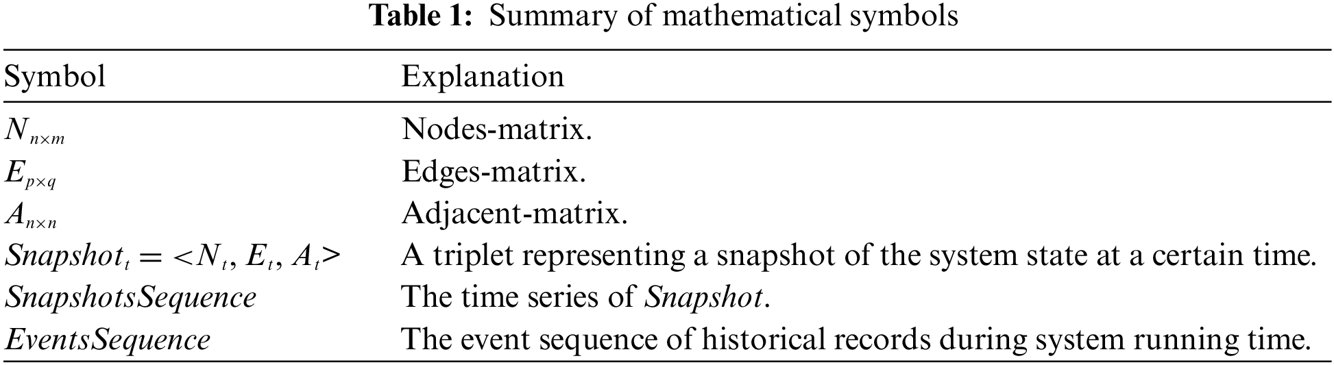
In this section, we first define several key concepts and then provide the objective of our research. For convenience, the main mathematical notations used in this section are summarized in Table 1.

The architecture of modern systems broadly adopts a complex distributed pattern. For such a distributed system, its structure can be naturally abstracted as a graph and can be denoted as GCloud. All the nodes in GCloud usually should follow a consistent granularity, e.g., services as nodes, processes as nodes, hosts as nodes, etc. The connections in GCloud correspond to interactions or dependencies between nodes, such as service invocation and message passing.

We are concerned not only with the topology but also with the properties of each element in it. The nodes and connections both have their properties. For example, on the nodes, there are resource usage and execution time, etc. On the connections, there are communication volume and transmission delays, etc. Therefore, multidimensional properties of either a “node” or “connection” can be represented by a vector x. We suppose that the quantity of nodes is n, each has m properties, there are p connections among the nodes, and each connection has q properties. Under the above settings, the following three matrices can characterize the state of the system.

Nodes-Matrix Nn×m: Each row of this matrix corresponds to a node of the system topology, and the row vector represents the node’s properties.

Edges-Matrix Ep×q: Each row of this matrix corresponds to a connection in the system topology, and the row vector represents the connection’s properties.

Adjacent-Matrix An×n: This matrix describes the node adjacency in the topological graph for the system.

After abstracting the system topologically and identifying the properties of the topological elements, to portray the system state more closely, the topological dynamics must be considered. The dynamics include two aspects as follows. (1) Structure dynamics: The system structure may change dynamically over time, e.g., the number of nodes and connections may change dynamically over time. (2) Property dynamics: The property values of each node and connection may change dynamically over time.

We use a triplet Snapshott = <Nt, Et, At> to represent a snapshot of the system state at a certain time. Then, by capturing the snapshots of the system state at a fixed interval period, we can get a time series SnapshotsSequencet0:tn = [Snapshott0, Snapshott1, . . . , Snapshottn]. If the observation interval period for SnapshotsSequence is valued appropriately, then SnapshotsSequence can be supposed to contain sufficient information for analyzing the system state from t0 to tn period.

During system operation, once anomaly events occur, such as service quality decline and unavailability, the professional staff submits event records in detail through structured or semistructured objects in various management information systems. It is worth highlighting that those records not only describe some basic information such as timestamp and location but also include the context and impact. Therefore, extracting worthwhile events from historical records is feasible and meaningful. We formally define the event sequence as EventsSequence = [e0, e1, . . . , en].

The relationship between EventsSequence and SnapshotsSequence is shown in Fig. 3. When we review the historical SnapshotsSequence and EventsSequence, we can assume that the SnapshotsSequence fragment earlier before an event is highly likely to contain some signs of the event occurrence. For example, as shown in Fig. 3, it is reasonable to assume that the series from t0 to t3 can reflect some signs of the occurrence of Event A.

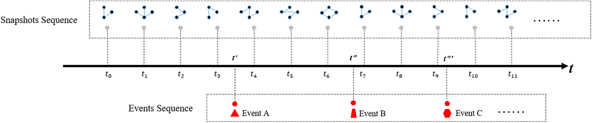
Figure 3: An example of the relation between SnapshotsSequence and EventsSequence

SnapshotsSequence is supposed to contain the integrity information reflecting the system state. Therefore, theoretically, it can be used to detect and predict the current and future state. We give the formal definition of the above statements as Eq. (1). The F function in Eq. (1) describes the research objective. It takes SnapshotsSequence as an input, and its output O is a vector of probability distributions that enumerates the types of events collected from EventsSequence with their corresponding probabilities of occurrence. O indicates the probability of an anomaly occurring in a short time from the current time t to the future t+t′. Alternatively, in some scenarios, it is acceptable to degrade the capability of the F function, whose output O is a binary result indicating the probability of being normal or not.

O=F(SnapshotsSequence(t−t″,t))(1)

The implementing techniques for the F function are open and diverse. Given a large amount of historical time series and event sequences as training samples, building a supervised machine learning model is advisable. In the following sections, we introduce our implementation for the F function called AD-DSTL.

4  Methodology

This section will provide a comprehensive overview of the model structure and methodological approach, followed by an in-depth analysis of critical issues.

4.1 The Overall Architecture

To implement the F function in Eq. (1), we propose AD-DSTL, an anomaly detection method for cloud systems based on dynamic spatiotemporal learning. The overall architecture of AD-DSTL is displayed in Fig. 4. Its input is the SnapshotsSequence, and its output is the prediction result. The input-output conforms to the Sequence2Sequence pattern. The input sequence element is Snapshott, which corresponds to the representation of the system state at time t. We know that Snapshott = <Nt, Et, At> includes information from both “nodes” and “connections” in the topology. Accordingly, we designed a model with dual pipelines, one of which is oriented to the nodes and the other is oriented to the connections. After processing independently, the two pipelines are combined through a fully connected layer to give the final result jointly.

Figure 4: The fundamental architecture of AD-DSTL

The core design idea of AD-DSTL is leveraging GCN [25] to extract the features hidden underneath the Snapshot, then passing the intermediate results to the downstream LSTMs [26], which remember the historical hidden features and combine historical dynamics with the latest input to produce the current prediction. In summary, GCN takes care of spatial feature extraction, while LSMT complements the capability of capturing temporal dynamics.

The common GCN only focuses on the features of nodes. In our opinion, the connection features are also important. It is necessary to find a way to process the connections using the same techniques processing the nodes to obtain the advantages of reusability and parallelism. Overall, there are several critical challenges and problems in the design of AD-DSTL. (1) How can the topology of the connections be reasonably characterized? (2) How can graph-level features be generated for systematic detection, even if the default output of the GCN is at the node level? (3) Do the dual LSTMs perform better than the single mode? Next, we will discuss the above issues.

4.2 GCN and Line Graph

As shown in Fig. 4, we use GCN to extract the state of the system topology at each moment t. GCN is a kind of deep learning technology designed for graph data. It is helpful when modeling the spatial dependence among metrics collected from interactive components. GCN draws lessons from the convolution operation in the frequency domain on an image by mapping the graph into the frequency space, performing the convolution operations, and then converting it back to the node space. The most commonly used GCN network was proposed by Kipf et al. [25], given a graph G and one layer of it can be formulated as Eq. (2), in which A is the adjacency matrix of G and Xl is the hidden representation of the node at the l layer, A~ = A + I is the adjacency matrix with the node’s loop inside, D~=∑i=0NA~ii is the degree matrix of A~, and σ(·) is the activation function.

Xl+1=σ(D−1/2A~D~−1/2XlWl)(2)

For the distributed cloud system mentioned in Section 3.1.1, a topological graph G can be naturally obtained from a physical perspective. Then, we can obtain the state of the topological nodes by calculating X in Eq. (2). If we had stopped here, then we would have ignored the status of all the connections among the nodes. However, these connections convey the internal interactions and are also critical to determining the state of the cloud system. Therefore, we adopted the method of line-graph conversion [27] to transform the original graph G into the corresponding line graph GE. Given an undirected graph G = (V, E), the line graph of G is an undirected graph GE = (E, F), in which there is an edge f ∈ F that connects the nodes e, e′ ∈ E if and only if there is a node v ∈ V such that both e and e′ are incident on v in G. If A is the adjacency matrix for G, then the adjacency matrix AE for GE can be deduced by Eq. (3).

AE=ATA−2I(3)

Through the line-graph conversion, the structure of the connections is preserved as much as possible. Consequently, we can reuse the same GCN method to extract the connection features. Fig. 4 shows that Phases 1 and 2 are divided into two parts. GCNN and GCNE are formulated as Eqs. (4) and (5), respectively.

GCNN:XNl+1=σ(D~N−1/2A~D~N−1/2XNlWNl)(4)

GCNE:XEl+1=σ(D~E−1/2E~D~E−1/2XElWEl)(5)

In Phase 1, illustrated in Fig. 4, two sets of inputs representing “nodes” and “connections” can be denoted by matrix SNt and matrix SEt, respectively. After the parallel calculation by GCNN and GCNE, the hidden features extracted from SNt and SEt can be denoted as FNt and FEt, respectively.

4.3 Graph-Level Features

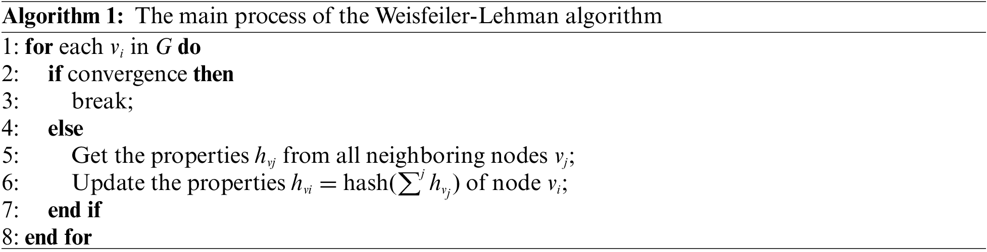
FNt and FEt are still one step away from the graph-level feature representation. Although joining all the nodes can be a way of obtaining the graph-level features, the problem with this method is that the topology of the graph evolves dynamically over time, so it is inadequate to stereotype the node features according to some static strategies (e.g., splicing node features in some fixed order). For a dynamic graph, it is crucial to ensure that the inductions at different moments follow an isomorphism principle. Namely, the nodes need to be ordered by a “consistent structural order.” For this purpose, we leverage the Weisfeiler-Lehman algorithm [28] to recognize the graph structure. The procedure of the one-dimensional Weisfeiler-Lehman algorithm is outlined in Algorithm 1, according to which we perform computing for each node in FNt and FEt. It assigns labels to the graph vertex by iterative computations, and in this way, the nodes with similar statuses or roles in different graphs will obtain the same labels. Then, by the labels, we can obtain an ordinal relationship to sort the nodes and join the ordered nodes to obtain the graph-level feature representation.

4.4 Dual LSTM Pipelines

LSTM is a special RNN network. Compared to an ordinary RNN, it implements a more sophisticated processor unit containing memory cells and several gate controllers. The memory cell maintains its state over time, and the gates control the information flow. LSTM usually consists of three gates: input gate, forget gate, and output gate. The gates are realized by the sigmoid function and dot multiplication operation. The general formulation of the gates can be expressed as g(x) = σ(Wx + b). Let i, f, and o represent the input gate, forget gate, and output gate, respectively. Let ⊙ represent an elementwise product, and let W and b represent the weight matrix and the offset vector of the network, respectively. The forward procedure of LSTM can be expressed as Eqs. (6) to (10), which are explained as follows.

At step t, the input and output vectors of the hidden layer of LSTM are xt and ht, respectively, and the memory unit is ct. The input gate is used to control how much the current input xt can flow into the ct. The value of the input gate is expressed by Eq. (6).

it=σ(Wixt+Wiht−1+bi)(6)

The forget gate controls which information should be kept or forgotten and in some way, avoids gradient disappearance or explosion. The value of the forget gate is expressed by Eq. (7). The forget gate can determine the influence of the last memory cell ct−1 on the current memory cell ct. The memory cell’s value is expressed by Eq. (8).

ft=σ(Wfxt+Wfht−1+bf)(7)

ct=ft⊙ct−1+it⊙tanh(Wcxt+Wcht−1+bc)(8)

The output gate controls how memory cell ct affects the current output value ht, that is, which part of the memory cell will be output at the time step t. The value of the output gate is expressed as Eq. (9), and the output ht of the LSTM at time t is expressed as Eq. (10).

ot=σ(Woxt+Woht−1+bo)(9)

ht=ot⊙tanh(ct)(10)

Jain et al. [29] mentioned that for sequences with irrelevant natures, higher accuracy could be obtained by using independently separated LSTMs. The explanation is that if two sequences are independent, then two LSTMs in isolation are a more natural way to correspond. As shown in Fig. 4, for AD-DSTL, we use two independent LSTMs for the two output sequences from GCNN and GCNE. We illustrate the architecture of the dual LSTMs in detail in Fig. 5.

Figure 5: The structure of dual LSTM pipelines

We can use a shorthand notation as Eq. (11) to denote the recurrent LSTM operation. Then, we pass the two graph feature streams (x1n . . . xTn) and (x1e . . . xTe) independently through LSTMN and LSTME, which are formulated as Eqs. (12) and (13), respectively. The fusion layer in Fig. 5 is formulated as Eqs. (14) and (15). We will verify the effectiveness of this approach in subsequent experiments.

(ht,ct)=LSTM(xt,ht−1,ct−1)(11)

(htn,ctn)=LSTMn(xtn,ht−1n,ct−1n)(12)

(hte,cte)=LSTMe(xte,ht−1e,ct−1e)(13)

et=tanh(Wf[htn;hte]+bf)(14)

yt=softmax(Wyet+by)(15)

5  Experimental Evaluation

In this section, we will show the experimental evaluation of AD-DSTL on four real datasets and provide an in-depth analysis of the process and results.

5.1 Datasets

We used four datasets, including three public datasets and one confidential dataset. The essential information is shown in Table 2.

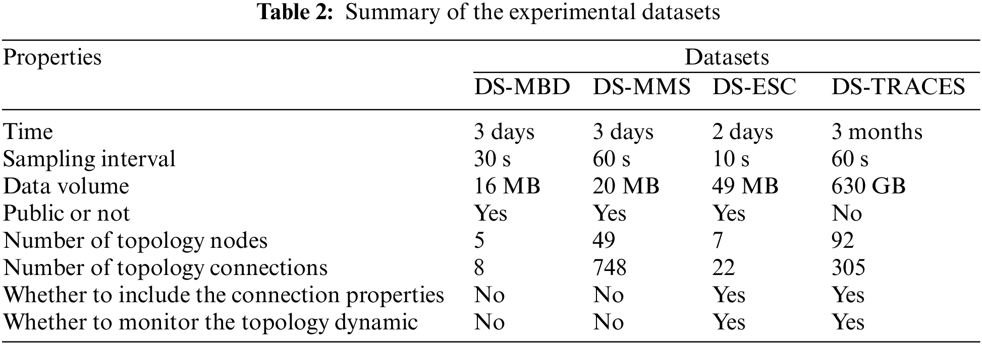
DS-MBD and DS-MMS are both from the work of He et al. [24]. DS-MBD is collected from a Hadoop cluster consisting of one master and four workers. DS-MMS is collected from a simulated microservice system called Hipster-Shop, which can be abstracted as a topology with 49 nodes and 748 connections. Notably, DS-MBD and DS-MMS only have monitoring data for node properties but not for connections. In addition, the system topology given by these two datasets is static.

DS-ESC is from the operational monitoring data of an elasticsearch cluster. The cluster consists of 7 nodes and provides data indexing services for software development and testing. We treat the processes of elasticsearch as topological nodes and the communications among the processes as topological connections. We call the Cluster-API provided by elasticsearch to collect the node states, which include the metrics of the OS, JVM, and various pooled resources for the process. We use the iftop command to capture the communications between specific ports held by the processes and acquire the number of network links and the amount of data exchanged. We have published DS-ESC for free access [8].

DS-TRACES is collected from the distributed invocation tracings for the microservices in a commercial bank. Its business background is complex financial processes involving various application systems in the banking field, such as channel systems, bus systems, core systems, credit systems, and batch operations. Taking the systems as the granularity for the nodes, DS-TRACES covers a total of 92 nodes, involving 305 connections. The monitored properties of the nodes include TPS, a 75% response time, memory usage, etc. The monitored properties of connections include the number of TIME_WAIT, number of messages, average latency, size of exchanged data, etc. DS-TRACES is confidential due to commercial reasons.

5.2 Performance Metrics

We use the F1-Score to evaluate the effectiveness of the anomaly detectors. The F1-Score is a commonly used evaluation metric for classification algorithms [30]. Its definition is shown in Eq. (16).

F1-Score=2×Precision×RecallPrecision+Recall(16)

The definitions of precision and recall are shown in Eqs. (17) and (18), respectively.

Precision=TP/(TP+FP)(17)

Recall=TP/(TP+FN)(18)

TP (true positive) represents the correct detection of an anomaly. FP (false positive) indicates that a normal state is mistaken for an anomaly. FN (false negative) indicates that an anomaly is mistaken for normal.

5.3 Experimental Setup

5.3.1 Comparison Methods

We compare AD-DSTL with several baseline anomaly detectors, including support vector machine (SVM) [31], GCN [25], LSTM [26], one-class support vector machine (OC-SVM) [32], LOF [12], and a topology-aware multivariate time series anomaly detector (TopoMAD) [24]. SVM, GCN, and LSTM are supervised methods. OC-SVM, LOF, and TopoMAD are unsupervised methods. SVM is a supervised learning method with the advantage of sound mathematical theory. LOF is a classical nonmachine learning anomaly detection method. Because of its simple implementation and good effect, it has been widely used. Since the AD-DSTL model is a composite model that combines GCN and LSTM, we selected both the original GCN and LSTM for comparison to confirm the effect of the compound. TopoMAD is also a composite deep learning model, but in contrast to AD-DSTL, it does not consider connections of the graph as inputs.

5.3.2 Experimental Environments and Parameters

To easily integrate AD-DSTL into a production environment's operations and maintenance (O&M) system, we implemented it using Deeplearning4j [33], a suite of tools for deploying and training deep learning models using the JVM. We implemented the GCN layer to Deeplearning4j and released the source code publicly [8]. All the experiments are conducted on a server with an Intel(R) Core(TM) i5-8250U CPU @ 1.6 GHz/1.80 GHz, 16 GB RAM, and Windows 11 installed.

The raw sampling intervals of MBD, MMS, ESC, and TRACES are 30, 60, 10, and 60 s, respectively. Because the sampling frequency is too high, we need to use a sliding window for coarse-grained aggregation. For DS-MBD, the sliding window size is 10 with a total period of 5 min; for DS-MMS, the sliding window size is 4 with a total period of 4 min; for DS-ESC, the sliding window size is 30 with a total period of 5 min; for DS-TRACES, the sliding window size is 4 with a total period of 4 min. The sliding step lengths are all one-half the size of the window, and the numeric metrics are all aggregated by calculating the average value. For the DS-MBD, DS-MMS, and DS-ESC datasets, for which the duration is two days, we used one day for training and the other day for testing. For the DS-TRACES dataset, we used a random filter to remove considerable bland data with meaningless repetition. Finally, the dataset was compressed to a total length of 4 days, in which two days were used for training and the others were used for testing. For each detector on each dataset, we repeated the tests ten times and then obtained the average score for comparison.

In the deep network of AD-DSTL, the GCN parts, including GCNN and GCNE are both set up with three layers, where the number of neurons in the input layer is equal to the length of the input dimensions, and the number of neurons in the middle and output layers are set as 64. Both LSTMs have one layer, and the hidden size of each layer is set to 128. The learning rate for the training of LSTMs was set to 10−3. The GCN and LSTM used for comparison are set up with the same parameters as the corresponding modules in AD-DSTL. For the TopoMAD algorithm, we use the reference configuration given in the original literature. LSTM, OC-SVM, SVM, and LOF cannot utilize the graph structure due to their limitations. For these methods, we concatenate all properties of the nodes and connections in a fixed order as the input. In addition, due to the lack of monitoring for the connection properties and topology dynamics in the datasets DS-MBD and DS-MMS, degradation strategies are adopted when using AD-DSTL to conduct experiments on those two datasets.

5.4 Overall Performance

We examined the overview performance of each algorithm. Fig. 6 shows the F1-score, precision, and recall of each tested algorithm on different datasets. Overall, the supervised methods work better than the unsupervised method, and the deep learning-based methods work better than the classic methods. That is as expected. However, we have not yet obtained results with high F1-scores. In the results, the comparatively better value of the F1-Score ranged from 0.6 to 0.7. AD-DSTL exhibits a more stable performance on all four datasets compared to other algorithms but is mostly still less than 0.7. The main reason for the low F1-scores is that all the precision values were generally not high. The precision was between 0.5 and 0.6 at best. Fortunately, most deep learning-based methods achieved relatively good recall performance, especially AD-DSTL, which acquired the highest recall value of 0.856.

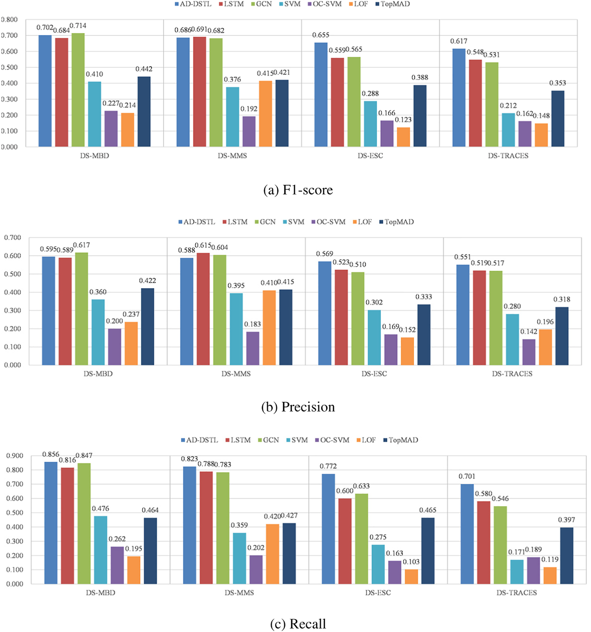
Figure 6: Comparing the best scores of each tested algorithm

Further comparing the results of all the tested algorithms, we can sense that the inherent nature of the dataset has a profound impact on the performance of algorithms. DS-MBD and DS-MMS are from the environments more inclined to simulations, while DS-ESC and DS-TRACES are collected in production environments. Therefore, there are more noisy and dirty data within DS-ESC and DSTRACES. Therefore, the F1-scores of each algorithm on DS-ESC and DS-TRACES are lower than those on DS-MBD and DS-MMS.

Regardless of the impact of the datasets, the methods based on deep learning were generally more stable. Compared to deep learning methods, SVM and LOF showed worse adaptability on complex datasets, and they could only perform well on simpler datasets.

The AD-DSTL algorithm shows the strongest robustness on different datasets. Although on the datasets DS-MBD and DS-MMS, the difference between the results of each algorithm is not obvious, when coming to the datasets DS-ESC and DS-TRACES, both of the other algorithms lag behind AD-DSTL evidently. The main reason for this is that there is only node status but no monitoring of connections in DS-MBD and DS-MMS, which degraded the capability of AD-DSTL and made AD-DSTL’s performance not much different from ordinary GCN and LSTM. However, additional connection monitoring helps AD-DSTL show distinctive advantages in DS-ESC and DS-TRACES.

Low precision is a matter of concern because it will result in ample false alerts. Therefore, it is necessary to answer the following two questions. (1) What is the reason for the low precision? (2) Are there any effective countermeasures against low precision?

The low precision is because of the noise and fluctuations in the datasets, which look like anomalies but are not. This phenomenon can affect both supervised and unsupervised methods. For unsupervised methods, noise may be classified as anomalies due to their anomaly scores being above the threshold. For supervised methods, the problem arises from the particular sampling means adopted due to sample imbalance. Since there are fewer anomaly samples and much more normal samples, some deliberate sampling balance techniques can easily lead to the sieving out of noise samples from the normal group. This causes the model to misclassify normal noise into an anomalous category.

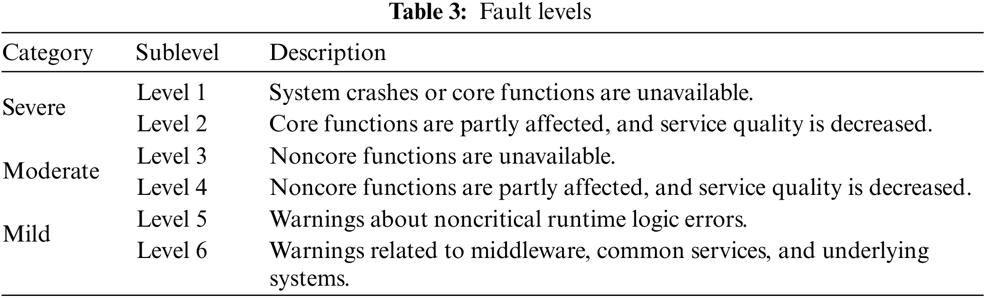
Low precision will bring great problems to system administrators, exhausting them in handling substantial fake alerts. Consequently, the anomaly detector loses its feasibility. In this regard, we further refine the verification experiments. Generally, in production management processes, the O&M specification classifies the severity level of the failure according to some dimensions, such as affected functions, impact scope, impact duration, and the number of affected businesses. For our experiment's datasets, DS-ESC and DS-TRACES, faults can be classified into three top categories with six fine-grained sublevels, as shown in Table 3. Accordingly, we proposed the following subdivided policies for anomaly labeling for the datasets DS-ESC and DS-TRACES. (1) Policy A: Keep all original anomaly labels. (2) Policy B: Only keep the anomalous labels in the categories of severe and moderate; the others are regarded as normal samples. (3) Policy C: Only keep the anomalous labels in serious categories; the others are regarded as normal samples.

Using the above three policies, three new datasets with different scopes of anomaly labeling can be obtained from the original DS-ESC and DS-TRACES datasets. We applied the AD-DSTL method to the newly derived datasets to verify the method’s effects. The results are shown in Table 4.

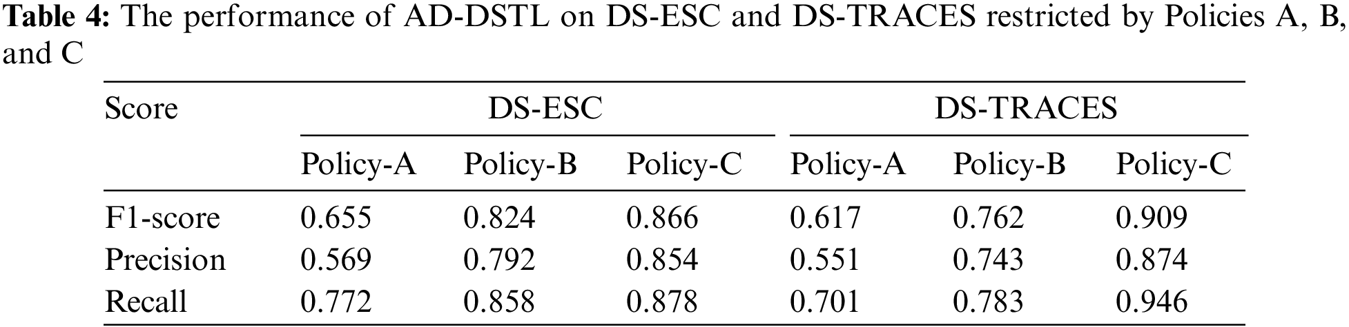
The validation results in Table 4 show that the AD-DSTL scores, especially the precision score, gradually increase with escalating failure levels. The main reason is that as the failure level increases, the specificity of the anomalies is relatively enhanced, so these anomalies can be different from normal random noise. The most evident manifestation is from the dataset DS-TRACES restricted with Policy C, where the performance of AD-DSTL is greatly improved. The trade-off of reducing the FP by increasing the detection level is consistent with the actual demands because higher-level faults tend to receive more attention in practice. Therefore, it is reasonable to consider detecting anomalies only at severe and moderate levels in practical applications.

In this paper, another critical problem is the generalization ability of AD-DSTL. AD-DSTL is a supervised method. For the sake of training efficiency, we chose to slice a subrange from the historical data for training rather than using the whole. Therefore, two implications need to be considered: (1) the selected training data cannot be guaranteed to be sufficiently comprehensive, and (2) the monitored system is evolving continuously, which may generate unknown conditions that have not appeared in history. This matters to the generalization ability of the detector. To investigate the generalization ability of AD-DSTL, we designed relevant evaluation experiments. The validation process is as follows. When training the model, we purposely partially take anomaly labels with the proportion of ρ from all. However, when validating the model, all the anomaly labels are included. In this way, we compare the F1-Score of the four supervised learning methods, including AD-DSTL, GCN, LSTM, and SVM, for the cases of ρ = 100%, ρ = 65%, and ρ = 35%. The results are shown in Fig. 7. As seen from the results, except for SVM showing ρ insensitivity because of its consistent ineffectiveness on the two datasets of DS-ESC and DS-TRACES, the performance of the remaining three declines as the ρ value decreases. Notably, from ρ = 100% to ρ = 65%, AD-DSTL’s F1-score has the smallest drop, especially on DS-ESC, which hardly diminishes. We believe that utilizing spatiotemporal factors in AD-DSTL is the fundamental reason for its superior generalization performance.

Figure 7: Results of the generalization ability test

Based on the above discussion, we can conclude the following.

1) For anomaly detection in complex systems, deep learning methods taking into account spatiotemporal factors show more advantages, especially in terms of robustness.

2) The validation demonstrates that AD-DSTL is of great practical value, focusing on two aspects. (a) After raising the fault grade, its performance is sufficient to achieve the application requirements. (b) It shows a strong generalization ability for the unknown types of anomalies that may constantly appear in production.

5.5 Effects of Topological Connections

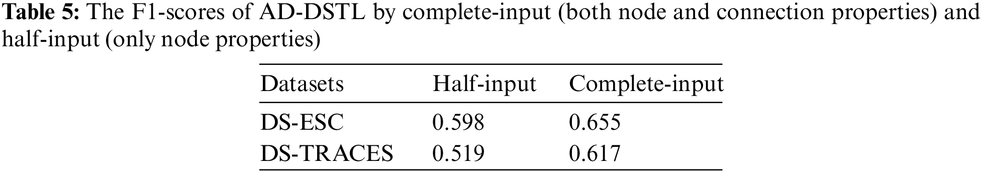
To investigate the effects of topological connections, we conducted the following experiments. We purposely ignored the topological connection properties using the DS-ESC and DS-TRACES datasets and only used the node properties. That is, AD-DSTL only received half of the input, and the other half of the input was null. The consequences under the above conditions are compared with the original, as shown in Table 5. When only retaining the input of the node part, DS-ESC and DS-TRACES both have significant drops in effectiveness compared to the original. This experiment confirms that topological connections have substantial effects on the research target.

5.6 Effects of Dual LSTMs

AD-DSTL intentionally designs architectures with dual LSTMs. The middle states are processed by two separate LSTMs in parallel before combining, rather than combining first and then input to a single LSTM. To clarify the practical effectiveness of this approach, we conducted experiments to compare the two different architectures mentioned above (single LSTM and dual LSTMs) on DS-ESC and DS-TRACES. The results are shown in Table 6. We can see that the dual LSTMs have a slight advantage. Therefore, if the training cost is acceptable, then dual LSTMs are a feasible and effective option.

6  Conclusion

We now summarize the main findings of our work and discuss some possible directions for future research.

6.1 Conclusion and Discussion

This paper targets the problem of anomaly detection for complex cloud systems. We propose a dynamic spatiotemporal learning method named AD-DSTL, which takes into account the collaborative structure and temporal dynamics in cloud systems. In the validation experiments, AD-DSTL demonstrates the strongest robustness compared to other baseline algorithms, and when raising the target exception level, both the recall and precision of AD-DSTL reach approximately 0.9. The experimental results demonstrated that AD-DSTL could satisfy the practical requirements. We have released part of the source code and datasets to facilitate future research [8].

In addition, we wish to discuss some important assumptions and limitations of this paper, as follows. First, the AD-DSTL model adopts a supervised learning technique design, assuming that labeled data required for training is readily available in the application environment. In the cloud service operation and maintenance scenario, various modern operation and maintenance platforms are usually constructed from which the required training data can be obtained. However, in most cases, the operation data management may lack standard work specifications and process practices. Consequently, the application of the AD-DSTL model may face diverse and complex data pre-processing issues. While this paper does not cover the data preparation, it should be noted that the actual application effect of the AD-DSTL model will be directly affected by this. Second, the design and validation of the AD-DSTL model focus on practical problems in its application context. The study examines crucial issues in model structure, topological edge parameters input, and topological dynamics. The AD-DSTL model is designed based on the principles of simplicity and effectiveness, aiming to facilitate easy application. Its design validity has been fully demonstrated through experimental results. However, regarding the abstract modeling of spatiotemporal dynamic learning problems, there may exist other variants of combined GCN and LSTM in AD-DSTL, such as using LSTM to initialize and maintain dynamic parameters in GCN rather than directly extracting system temporal state features. Although this paper does not delve into these issues in-depth, a comprehensive generalization of related technical theories could enhance understanding of the advantages of model design in depth.

6.2 Future Work

For future work, we will continue to focus on the following issues. (1) This paper has only validated the AD-DSTL model on just four datasets. Next, it is suggested to collect more validation datasets from realistic environments and further research the optimization for various hyperparameters of AD-DSTL. (2) We assumed that labeled data could be obtained conveniently. However, that assumption may not represent all cases, so it is worthwhile to research how to evolve toward semi-supervised or unsupervised learning schemes. (3) The location and interpretability of anomalies deserve more attention. In particular, it would be valuable if it could suggest the anomaly time, location, and even cause in the spatiotemporal context.

Funding Statement: This work was supported by the National Key Research and Development Program of China (2022YFB4500800).

Conflicts of Interest: The authors declare that they have no conflicts of interest to report regarding the present study.

References

1. A. Aggarwal, P. Dimri and A. Agarwal, “Statistical performance evaluation of various metaheuristic scheduling techniques for cloud environment,” Journal of Computational and Theoretical Nanoscience, vol. 17, no. 9–10, pp. 4593–4597, 2020. [Google Scholar]

2. Y. Li, Z. M. (jack) Jiang, H. Li, A. E. Hassan, C. He et al., “Predicting node failures in an ultra-large-scale cloud computing platform: An AIOps solution,” ACM Transactions on Software Engineering and Methodology, vol. 29, no. 2, pp. 1–24, 2020. [Google Scholar]

3. P. Notaro, J. Cardoso and M. Gerndt, “A survey of AIOps methods for failure management,” ACM Transactions on Intelligent Systems and Technology, vol. 12, no. 6, pp. 1–45, 2021. [Google Scholar]

4. Y. Xu, K. Sui, R. Yao, H. Zhang, Q. Lin et al., “Improving service availability of cloud systems by predicting disk error,” in USENIX Annual Technical Conf., Boston, MA, USA, pp. 481–494, 2018. [Google Scholar]

5. Y. Xu, N. Chen, R. Huang and H. Zhang, “KPI data anomaly detection strategy for intelligent operation and maintenance under cloud environment,” in Intelligent Information Processing IX-10th IFIP TC 12 Int. Conf., Nanning, China, pp. 311–320, 2018. [Google Scholar]

6. S. Zhang, C. Zhao, Y. Sui, Y. Su, Y. Sun et al., “Robust KPI anomaly detection for large-scale software services with partial labels,” in 32nd IEEE Int. Symp. on Software Reliability Engineering, Wuhan, China, pp. 103–114, 2021. [Google Scholar]

7. H. Haugerud, M. Sobhie and A. Yazidi, “Tuning of elasticsearch configuration: Parameter optimization through simultaneous perturbation stochastic approximation,” Frontiers in Big Data, vol. 5, no. 1, pp. 686416, 2022. [Google Scholar] [PubMed]

8. AD-DSTL, 2022. [Online]. Available: https://github.com/yumg/adcd [Google Scholar]

9. B. Steenwinckel, P. Heyvaert, D. D. Paepe, O. Janssens, S. V. Hautte et al., “Towards adaptive anomaly detection and root cause analysis by automated extraction of knowledge from risk analyses,” in Proc. of the 9th Int. Semantic Sensor Networks Workshop co-located with 17th Int. Semantic Web Conf., Monterey, CA, United States, pp. 17–31, 2018. [Google Scholar]

10. N. Stojanovic, M. Dinic and L. Stojanovic, “A data-driven approach for multivariate contextualized anomaly detection: Industry use case,” in IEEE Int. Conf. on Big Data, Boston, MA, USA, pp. 1560–1569, 2017. [Google Scholar]

11. N. Ishaq, T. J. H. Iii and N. M. Daniels, “Clustered hierarchical anomaly and outlier detection algorithms,” in IEEE Int. Conf. on Big Data, Orlando, FL, USA, pp. 5163–5174, 2021. [Google Scholar]

12. O. Alghushairy, R. Alsini, T. Soule and X. Ma, “A review of local outlier factor algorithms for outlier detection in big data streams,” Big Data and Cognitive Computing, vol. 5, no. 1, pp. 1, 2021. [Google Scholar]

13. S. Ul Amin, M. Ullah, M. Sajjad, F. A. Cheikh, M. Hijji et al., “EADN: An efficient deep learning model for anomaly detection in videos,” Mathematics, vol. 10, no. 9, pp. 1555, 2022. [Google Scholar]

14. S. Gadal, R. Mokhtar, M. Abdelhaq, R. Alsaqour, E. S. Ali et al., “Machine learning-based anomaly detection using K-mean array and sequential minimal optimization,” Electronics, vol. 11, no. 14, pp. 2158, 2022. [Google Scholar]

15. T. Ergen and S. S. Kozat, “Unsupervised anomaly detection with LSTM neural networks,” IEEE Transactions on Neural Networks and Learning Systems, vol. 31, no. 8, pp. 3127–3141, 2020. [Google Scholar] [PubMed]

16. K. Ding, J. Li, R. Bhanushali and H. Liu, “Deep anomaly detection on attributed networks,” in Proc. of SIAM Int. Conf. on Data Mining, Calgary, Alberta, Canada, pp. 594–602, 2019. [Google Scholar]

17. G. Pang, C. Shen, L. Cao and A. van den Hengel, “Deep learning for anomaly detection: A review,” ACM Computing Surveys, vol. 54, no. 2, pp. 1–38, 2022. [Google Scholar]

18. C. Wang, H. Zhou, Z. Hao, S. Hu, J. Li et al., “Network traffic analysis over clustering-based collective anomaly detection,” Computer Networks, vol. 205, no. 3, pp. 108760, 2022. [Google Scholar]

19. M. S. Islam, W. Pourmajidi, L. Zhang, J. Steinbacher, T. Erwin et al., “Anomaly detection in a large-scale cloud platform,” in 43rd IEEE/ACM Int. Conf. on Software Engineering: Software Engineering in Practice, Madrid, Spain, pp. 150–159, 2021. [Google Scholar]

20. M. Du, F. Li, G. Zheng and V. Srikumar, “DeepLog: Anomaly detection and diagnosis from system logs through deep learning,” in Proc. of ACM SIGSAC Conf. on Computer and Communications Security, Dallas, TX, USA, pp. 1285–1298, 2017. [Google Scholar]

21. J. Soldani and A. Brogi, “Anomaly detection and failure root cause analysis in (micro) service-based cloud applications: A survey,” ACM Computing Surveys, vol. 55, no. 3, pp. 1–39, 2022. [Google Scholar]

22. C. Zhang, D. Song, Y. Chen, X. Feng, C. Lumezanu et al., “A deep neural network for unsupervised anomaly detection and diagnosis in multivariate time series data,” in The Thirty-Third AAAI Conf. on Artificial Intelligence, Honolulu, Hawaii, USA, pp. 1409–1416, 2019. [Google Scholar]

23. W. Cheng, J. Ni, K. Zhang, H. Chen, G. Jiang et al., “Ranking causal anomalies for system fault diagnosis via temporal and dynamical analysis on vanishing correlations,” ACM Transactions on Knowledge Discovery from Data, vol. 11, no. 4, pp. 1–28, 2017. [Google Scholar]

24. Z. He, P. Chen, X. Li, Y. Wang, G. Yu et al., “A spatiotemporal deep learning approach for unsupervised anomaly detection in cloud systems,” IEEE Transactions on Neural Networks and Learning Systems, vol. 1, no. 1, pp. 1–15, 2020. [Google Scholar]

25. T. N. Kipf and M. Welling, “Semi-supervised classification with graph convolutional networks,” in 5th Int. Conf. on Learning Representations, Toulon, France, pp. 24–26, 2017. [Google Scholar]

26. S. Hochreiter and J. Schmidhuber, “Long short-term memory,” Neural Computation, vol. 9, no. 8, pp. 1735–1780, 1997. [Google Scholar] [PubMed]

27. O. D. La Cruz Cabrera, M. Matar and L. Reichel, “Edge importance in a network via line graphs and the matrix exponential,” Numerical Algorithms, vol. 83, no. 2, pp. 807–832, 2020. [Google Scholar]

28. N. T. Huang and S. Villar, “A short tutorial on the Weisfeiler-Lehman test and its variants,” in IEEE Int. Conf. on Acoustics, Toronto, ON, Canada, pp. 8533–8537, 2021. [Google Scholar]

29. A. Jain, A. Singh, H. S. Koppula, S. Soh and A. Saxena, “Recurrent neural networks for driver activity anticipation via sensory-fusion architecture,” in IEEE Int. Conf. on Robotics and Automation, Stockholm, Sweden, pp. 3118–3125, 2016. [Google Scholar]

30. D. Fourure, M. U. Javaid, N. Posocco and S. Tihon, “Anomaly detection: How to artificially increase your F1-score with a biased evaluation protocol,” in ECML PKDD, Bilbao, Basque Country, Spain, pp. 3–18, 2021. [Google Scholar]

31. M. Baldomero-Naranjo, L. I. Martínez-Merino and A. M. Rodríguez-Chía, “A robust SVM-based approach with feature selection and outliers detection for classification problems,” Expert Systems with Applications, vol. 178, no. 1, pp. 115017, 2021. [Google Scholar]

32. Y. Ji and H. Lee, “Event-based anomaly detection using a one-class SVM for a hybrid electric vehicle,” IEEE Transactions on Vehicular Technology, vol. 71, no. 6, pp. 6032–6043, 2022. [Google Scholar]

33. Deeplearning4j, 2022. [Online]. Available: https://github.com/eclipse/deeplearning4j [Google Scholar]