Integrated Generative Adversarial Network and XGBoost for Anomaly Processing of Massive Data Flow in Dispatch Automation Systems

1  Introduction

With the acceleration of power grid construction and the expansion of its scale, various dispatch automation systems have successively been built. Moreover, business interactions between the various systems of local dispatching and county dispatching have become more frequent with the power dispatching data network emerging. What followed was an exponential growth in the amount of power dispatching data, along with the era of big data in the power dispatching data networks. To meet the needs of a smart grid, an intelligent dispatch system should have a more comprehensive and accurate data acquisition system, with a powerful intelligent security early warning function. It should also, and pay attention to the coordination of system safety and economy in dispatch decisions. Thus, when the system fails, it can quickly Diagnose faults and provide fault recovery decisions.

At present, with the increase in dispatch data, the monitoring data of electric power dispatch has the nature of a large, rapid, and continuous sequence that has the characteristics of streaming data. Additionally, changes in the distribution of streaming data can introduce concept drift problems. Current anomaly detection methods for dispatching data mainly include methods such as threshold judgment based on a single system and analysis methods based on static offline data. The threshold judgment method based on a single system has the following limitations: (i) the utilization rate of equipment information and the correct rate of state evaluation are low; (ii) it is difficult to detect the latent faults and fault types of equipment; (iii) the thresholds in relevant standards are fixed and it is difficult to adapt to the differences in equipment operating conditions. The analysis method based on static offline data has issues that include not being closely integrated with the operation system, being unable to quickly reflect the operating status of the system, and being unable to detect anomalies in time [1].

In the application scenario of grid, power big data has the characteristics of sequence, timing, and large number, whereas the number of abnormal samples generated is relatively very small, and many anomalies can be subdivided into smaller abnormalities. Therefore, in this paper we propose a novel anomaly detection method of massive data flow in dispatch automation system. The contributions are as follows:

1.    First, we introduce GAN to the field of online data volume parsing and rapid anomaly identification of dispatch automation systems, combining GAN with classical fault diagnosis methods. With GAN, a large number of reliable labeled datasets are obtained for the training of fault diagnosis models based on a few labeled data points, which not only greatly reduces the time required for manually labeling the training data but also improves the accuracy of the fault diagnosis models.

2.    Then we propose a two-step detection algorithm. In the first step, the XGBoost algorithm is selected to reduce the dimensionality of the data, remove redundant data, select the optimal combination of features for the input parameters in the fault detection phase, and divide the final processed data into a training set and test set for the training of the XGBoost fault detection model used to obtain the diagnostic results of the large class of anomalies. Then the data processed in the first step is then input into the joint CNN+LSTM model for fine-grained analysis to detect the small class of anomalies. This takes advantage of the fact that CNN can automatically extract features from massive data and that LSTM can handle time series variations to combine the two algorithmic models to better handle various grid anomalies. The two-step detection process integrates the characteristics of the grid data and fully utilizes the advantages of various algorithmic models to obtain optimal diagnostic results.

3.    Simulation results have shown that this method can achieve accurate and efficient grid fault diagnosis and prediction. This method can discover safety hazards in the dispatch automation system in real time and lays a good foundation for the safe, stable, high-quality, and economical operation of the power grid.

The remainder of this paper is structured as follows: the second part presents the related work,the third part presents the system model,the fourth part discusses the proposed fault diagnosis method, the fifth part contains the experimental results and analysis, and the sixth part contains the conclusion.

2  Related Work

In the field of smart grid anomaly detection, scholars from various countries have recently used machine learning to actively explore, thereby achieving certain research results. For example, Ying et al. [2] combined the rule-based method with the nearest neighbor-based method to design an anomaly detection method for detecting network traffic in power systems. Also, Wang et al. [3] and Yang et al. [4] used existing SVM as well as k-means anomaly detection methods to perform anomaly diagnosis for the characteristics of power system data. Furthermore, Pang et al. [5] combined grid structure with data characteristics to establish an anomaly detection framework based on the spectral theory and analyzed its residuals. Additionally, Xu et al. [6] proposed an anomaly user behavior detection method based on CNN-GS-SVM, which is better than the traditional method in terms of accuracy and efficiency. Yang et al. [7] combined LightGBM with an improved LSTM model for the anomalous power usage detection method, with their experimental results indicating that this method had better anomaly detection accuracy and anomaly classification accuracy. Also, Li et al. [8] used LSTM to extract features and used a traffic anomaly detection method based on an improved SVM-embedded decision tree model, which has higher accuracy when compared to the traditional method. All of these methods were used in combination with existing methods for the characteristics of power data.

Other scholars have researched the time series problem of the power system. For example, Ul Amin et al. [9] proposed an efficient Deep Learning Model for anomaly detection in video streams. The model takes video segmentations as input using a shot boundary detection algorithm and uses a Convolutional Neural Network (CNN) to extract salient spatiotemporal features. Lastly, Long Short-Term Memories (LSTM) cells are employed to learn spatiotemporal features from a sequence of frames per sample of each abnormal event for anomaly detection. The combination of CNN and LSTM greatly improves the classification accuracy of anomalies data and the effectiveness of the training process. However, the above literatures have a limitation that is the lack of training and testing data. Therefore, we propose the use of GAN to generate data samples for training the classification model. Yang et al. [10] quantified the historical data of transmission and substation equipment using self-organizing neural networks, mined the changing patterns of data over time, and combined autoregressive models and DBSCAN clustering methods to establish anomaly models. After segmenting the power data time series into linear representations, Pei et al. [11] innovatively combined the Venn diagram in graph theory with the nearest neighbor distribution density in the nearest neighbor to achieve the goal of a high detection rate and low false alarm rate. Moreover, Wang et al. [12] conducted hierarchical analyses and discussions on the importance of each dimension of power system data and then combined the nearest neighbor method for electricity theft monitoring. Pan et al. [13] used spectral theory to analyze the composition structure of satellite power system data and combined association rules and clustering to learn data laws and build models for real-time detection. However, the aforementioned methods are more for time-invariant power system data and are not applicable in power systems with multiple data types and large volumes, while research on power system anomaly detection methods with conceptual drift remains at the exploration stage. Additionally, the dimensional size of data is one of the most important factors affecting the performance of anomaly detection methods, while the number of data dimensions that must be monitored by the power dispatch automation system business depends on the type of business. Therefore, it is necessary to use detection methods that can have good detection effects in all dimensions [14,15].

Based on the aforementioned research on grid fault diagnosis methods, it can be concluded that traditional grid fault diagnosis methods has the following drawbacks. First, insufficient data for analysis. Second, having difficulty in finding hidden problems. Third, requiring a large number of manually labeled training datasets which is time-consuming and labor-intensive [16]. Additionally, grid faults will become more diverse and the identification of grid faults will rely on more Key Performance Indicators (KPIs). Thus, it is necessary to consider how to obtain a large number of reliable datasets in a complex power grid. The most common practice involves extracting information from labeled cases of known faults, with the extracted dataset being used to obtain fault diagnosis strategies through supervised learning. However, few histories are available since experts do not tend to collect the values of KPIs and the tags associated with the faults they solve. In particular, there are not many faults in the real network and there are not many labeled cases for each particular fault. As a result, the historical data available from the real network is not rich enough to achieve the results achieved by using supervised techniques for building a diagnostic system. Moreover, the problem of not having sufficient historical data can be solved by generative adversarial networks (GANs).

In recent years, GANs have been widely used in the fields of computer vision, image recognition, and natural language processing as a typical method for implementing artificial intelligence, thereby allowing people to appreciate its amazing ability in dealing with complex problems. A GAN consists of two independent deep networks [17]: a generator and a discriminator. The generator accepts a random variable that obeys the pg distribution of random variables and maps it to the data distribution. The discriminator outputs 1 and 0 to distinguish the real samples from the generated ones, respectively. During the GAN training process, samples are generated and classified separately using the generator and discriminator to adversarially improve the performance. Experimental results have demonstrated the potential of this framework by using this method for the recognition of MNIST handwritten datasets. However, Wang [18] experienced some problems in the actual training process, such as training difficulties and a lack of diversity in the generated samples, among other issues. The authors of [19,20] proposed Wasserstein GAN (WGAN) to address the problems in [18], and the simulation results showed that the framework can solve the problem of GAN training instability and ensure the diversity of the generated samples. Mowlaei et al. [21] proposed an algorithm named Population-Scale Genomic Data Augmentation based on Conditional Generative Adversarial Networks to enhance the amount and diversity of genomic data by transforming samples already in the data rather than collecting new samples. Zhang [22] first explained the reasons for GAN training instability from a theoretical perspective. Then, Wasserstein distance was introduced to replace Jensen-Shannon (JS) scatter and Kullback Leibler (KL) scatter and used as an optimization objective. Compared to the KL scatter and JS scatter in the original GAN, the WGAN solves the gradient vanishing problem that exists in the original GAN. Currently, GANs are mainly applied in the field of computer vision [23]; however, they are rarely used in communication systems.

The current anomaly detection methods for power dispatching data mainly include simple threshold determination based on a single system and analysis methods based on static offline data. The simple threshold determination method based on a single system has following limitations. On the one hand, the equipment information utilization rate and status evaluation accuracy are low, and on the other hand, it is difficult to detect latent faults and fault categories of the equipment. Moreover, the fixed threshold in relevant standards and regulations is difficult to combine with the differences in equipment operating conditions. The analysis method based on static offline data is not closely connected with the production and operation system, and cannot quickly reflect the system operation status and timely detect abnormal phenomena. Therefore, this paper uses machine learning algorithm to realize anomaly detection of massive information flow.

3  System Model

In this paper, we consider the power dispatch automation system presented in Fig. 1, including the main network and the distribution network with separate acquisition workstations. Among them, the main network data acquisition workstation mainly collects the message data in the main network; that is, the message data sent from the remote control device of the factory station to the front-end processor of the master station. The main network data acquisition workstation is mainly connected to the front switch through the mirror port, and the front switch is connected to the front-end processor, while the two front-end processors are used as a backup for each other. Connecting the two inter-standby front switches can make the collected data more comprehensive and complete while preventing the data source from being completely cut off when the data dispatching network equipment fails or undergoes maintenance. The distribution network data collection workstation mainly collects the message data in the distribution network, which is sent by the distribution automatic terminal of the plant station. The plant station distribution automatic terminal sends data up to the main station in the security access zone, while the message data is gathered to the security zone switch through isolating devices and the distribution network data collection workstation is connected to the security zone switch through the mirror port. Based on big data and Artificial Intelligence (AI) technology, the anomaly identification and diagnosis servers perform the intelligent identification, diagnosis, and prediction of faults in the power dispatching automation system.

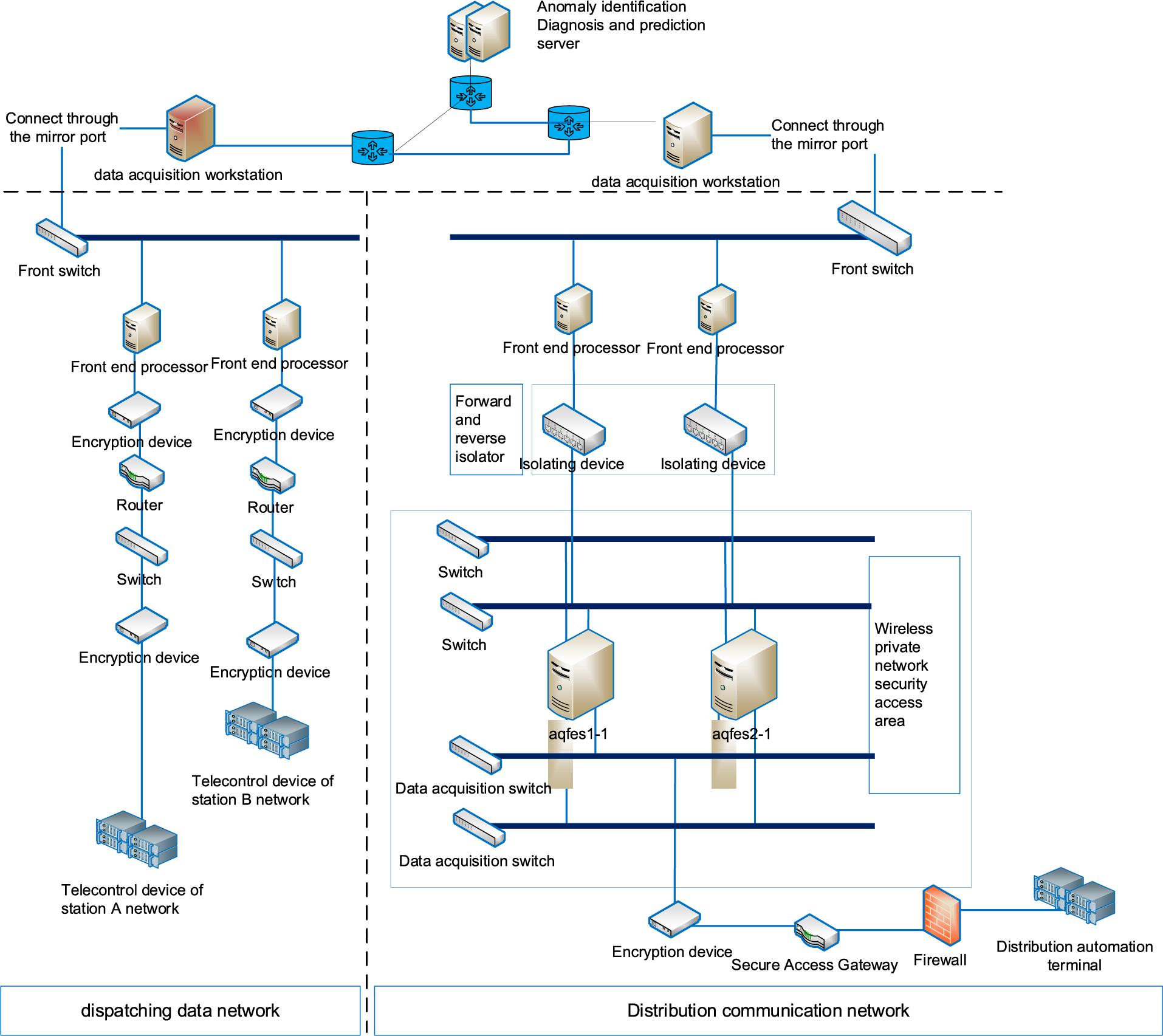
Figure 1: Power automatic dispatching system

In this paper, we study the characteristics, discrimination methods, and prediction techniques for anomalies in massive information flow. First, we summarize the statute message structure and application function classification. Second, we study the anomaly characteristics and fault analysis of massive information flow to classify the dispatching flow anomaly. Finally, we implement massive information flow anomaly identification, diagnosis, and prediction using a machine learning algorithm.

According to the characteristics of grid anomaly data, we designed an anomaly feature and fault discrimination framework based on massive information streams (see Fig. 2). Firstly, for the data generated by the power dispatching data network, we use the lossless acquisition to get the message information stream. For the problem of insufficient anomalous data, we use WGAN-GP to obtain enough reliable datasets with labels for the training of fault diagnosis models based on a few labeled data points. Then, a two-step detection process was designed for the known anomaly characteristics of the power grid. In the first step of this process, the generated samples are input into the XGBoost recognition system to identify the large class of anomalies. Then, the data processed in the first step are input into the joint CNN+LSTM model for fine-grained analysis to detect the small class of anomalies.

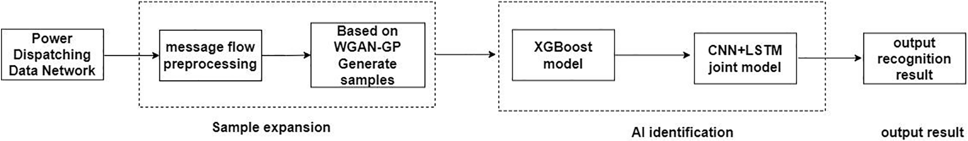
Figure 2: Framework for anomaly classification and fault detection techniques in massive information flow

Fig. 2 describes the complete process of anomalies detection in power dispatching data network. First, we implement a preprocessing step on the collected data to remove irrelevant features which may have a great influence to the classification module if had not been done. Second, we use the WGAN-GP algorithm to expand samples. Then, the generated samples are put into the XGBoost recognition system to classify the large class anomalies. In the end, samples that have not been identified will be put into the joint CNN+LSTM model to realize the classification of small class samples.

The real-time attributes and reliability of the dispatching service information flow directly affect the realization of each service function, which means that transmission delay should be guaranteed to be within the required time range, with no packet loss or retransmission in case of loss. Due to some problems in the design, setting, and maintenance of channels, equipment, and systems that cannot be eliminated, “four remote” anomalies may occur. Some of these anomalies are in response to the real state of the site, while others are caused by various errors. Notably, these anomalies result in major issues related to the operation of a power system and its maintenance personnel [24].

According to the formation mechanism and characteristic quantity of dispatching service information flow anomaly for classification, this paper classifies the data flow fault anomaly into functional anomaly, timeliness anomaly, communication anomaly, and integrity anomaly. The details are presented in Fig. 3.

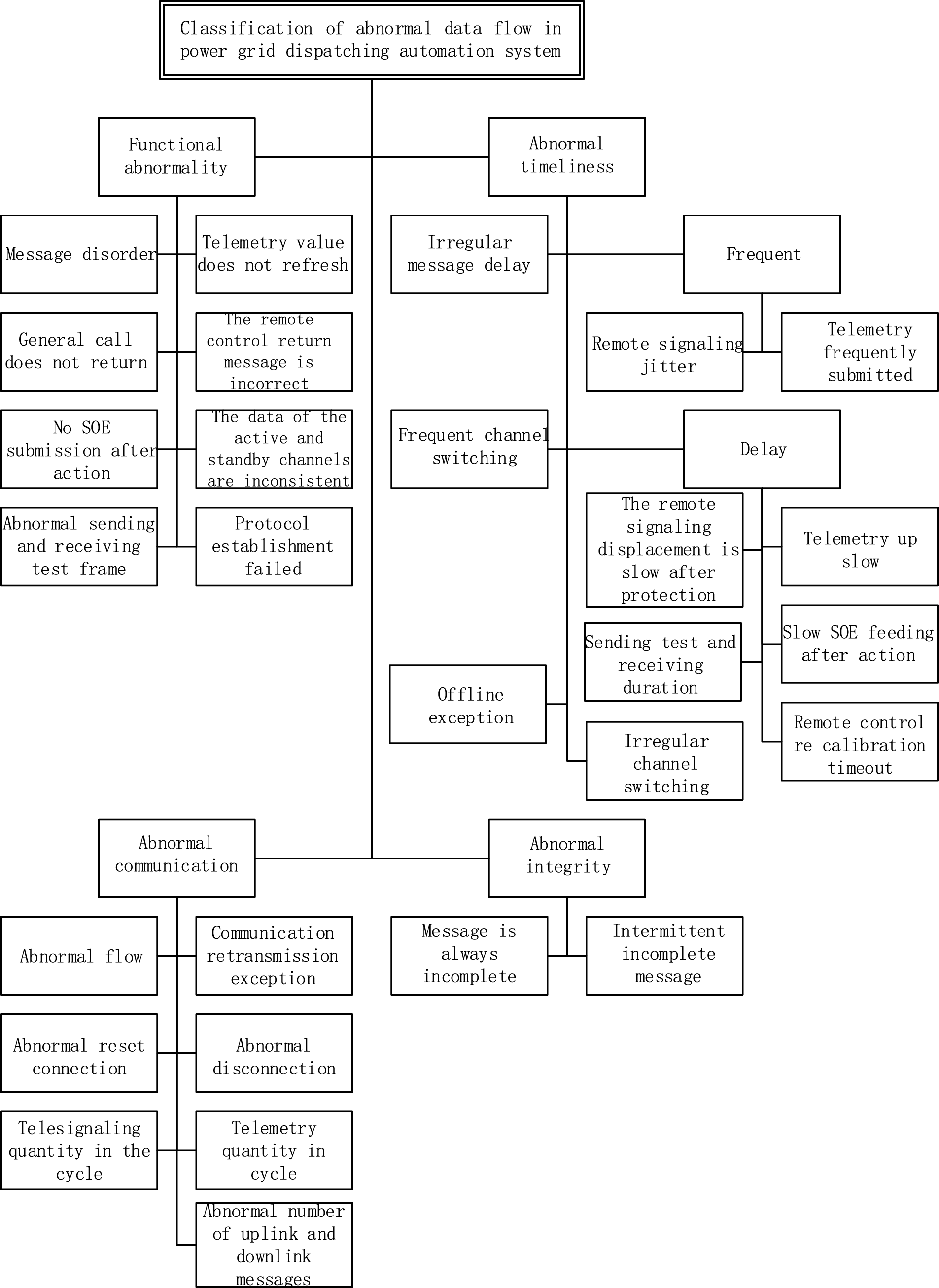
Figure 3: Classification of data flow faults

(1) Functional anomalies

Functional anomalies contain the following cases. (a) Message disorder: the message is disassembled since multiple 104 messages return confusing serial numbers or there are missing messages. (b) Telemetry values are not refreshed: the telemetry value in the telemetry message has not changed for a long time. (c) General recall not to return: no message is returned after sending the general call command. (d) No SOE upload after action: the Sequence of Event (SOE) signal is not sent up after the protection signal is actuated. (e) Send and receive test frame anomalies: when there is no information interaction between the master and the distribution terminal, the master does not send test frames and the terminal side sends test frames for a long time without any messages from the master in between. In the 104 protocol, if the master does not send a message after a certain period or the terminal does not send any messages, then both sides can send test frames by sending U frames at the frequency. (f) Incorrect remote return message: the remote preset command should return “preset successfully”, but instead returns “execute successfully.” Or the remote execution command should have returned “execute successfully,” but instead returned “preset successfully.” (g) Inconsistent master and standby channel data: messages on the master channel are inconsistent with the messages on the standby channel, there are more or fewer messages, or the point number values sent up are inconsistent. (h) Failure to establish a statute: Transmission Control Protocol (TCP) is successfully established, the master sends the 104 statutes to start command (68 04 07 00 00 00), the distribution terminal does not respond (68 04 0b 00 00 00), and application layer connection establishment fails.

(2) Time-sensitive anomalies

Time-sensitive anomalies contain the following cases. (a) Frequently sending telecommunication jitter: The telecommunication signals are sent frequently for a short period, resulting in the failure of the main station front to respond and the signal not changing. Frequent telemetry upload: A large number of telemetry signals are frequently uploaded over a short period. (b) Frequent channel switching: the active channel is frequently switched, with frequent switching of Internet Protocol Address (IP) occurring in the messages. (c) Delays. (i) Slow telecommunications change after protection: long change duration for telecommunication changes after protection actions. (ii) Slow telemetry upload: telemetry signal upload time exceeds the standard duration. (iii) Transmit test and receive duration: automatically detects the time delay between test frame transmission and test frame reception; a time delay greater than the threshold value is considered abnormal. (iv) Slow SOE feed after action: there is an SOE signal feed after the action, but it is not sent until long after the shift has occurred. (v) Time extension between the remote process preset and the preset confirmation message. (vi) Time delay between the preset and preset confirmation message of the remote control process and the time delay between the execution and execution confirmation message is automatically detected, while a time delay greater than the threshold value is considered an exception. (d) Irregular channel switching: channel switching is infrequent and irregular (not a regularity that can be caused by normal operation). (e) Offline anomalies: refreshing the online/offline status of power distribution terminals based on TCP. This detects the offline status of the power distribution terminal and can periodically count the number of times the power distribution terminal is offline, as well as the length of time it is offline [25]. The number of offline times and abnormality thresholds for offline duration can be set, with abnormalities being determined when the thresholds are exceeded.

(3) Communication anomalies

Communication anomalies contain the following cases. (a) Flow anomalies: traffic is counted over a certain period based on IP address, and an abnormality is determined if the traffic exceeds the set threshold or if the traffic curve is abnormal. (b) Communication retransmission anomalies: count the number of TCP retransmission messages over a certain period and the total number of TCPs transmitted. The TCP retransmission rate over this period is calculated and compared to a TCP retransmission rate threshold that can be set (e.g., 30%). If the retransmission rate is greater than the set threshold, a “communication link retransmission rate too high” alert is provided, which may affect service data transmission. (c) Reset connection anomalies: after analyzing the TCP layer message, the master initiates a TCP connection request (SYN) to the distribution terminal. Subsequently, the distribution terminal resets the TCP connection with the flag bit identified as Reset (RST), with an exception being determined thereafter. (d) Disconnection anomalies: when the TCP layer message is analyzed and the master initiates a TCP connection request (SYN) to the distribution terminal and the distribution terminal subsequently disconnects the TCP connection with the flag bit (identified as Finish (FIN)), an exception is determined. (e) Anomalous number of remote signals in the cycle: the number of telegrams sent from the distribution terminal during the period is counted and the threshold value is respectively set. If the number of telegrams is greater than the threshold value, it is considered abnormal. (f) Anomalous number of uplink messages: the number of application layer messages sent by the master station and distribution terminal during the period is counted separately, the threshold value is set separately, and a value greater than the threshold value is considered abnormal. (g) Anomalous number of downlink messages: the numbers of application layer messages sent by the master station and distribution terminal over a certain period are counted separately, the threshold value is set separately, and a value greater than the threshold value is considered abnormal. (h) Periodic offline anomalies: the TCP transmission process reset flag RST is detected, the number of reset messages is counted, and the number of times exceeding the threshold value is considered abnormal. Detects frequent resetting of the distribution terminal and the existence of the periodic offline phenomenon, while the length of each offline time is fixed.

(4) Integrity anomalies

Integrity anomalies contain (a) messages that are always mutilated (i.e., missing parts of their content); (b) intermittently incomplete messages (i.e., incomplete or complete messages are sent intermittently).

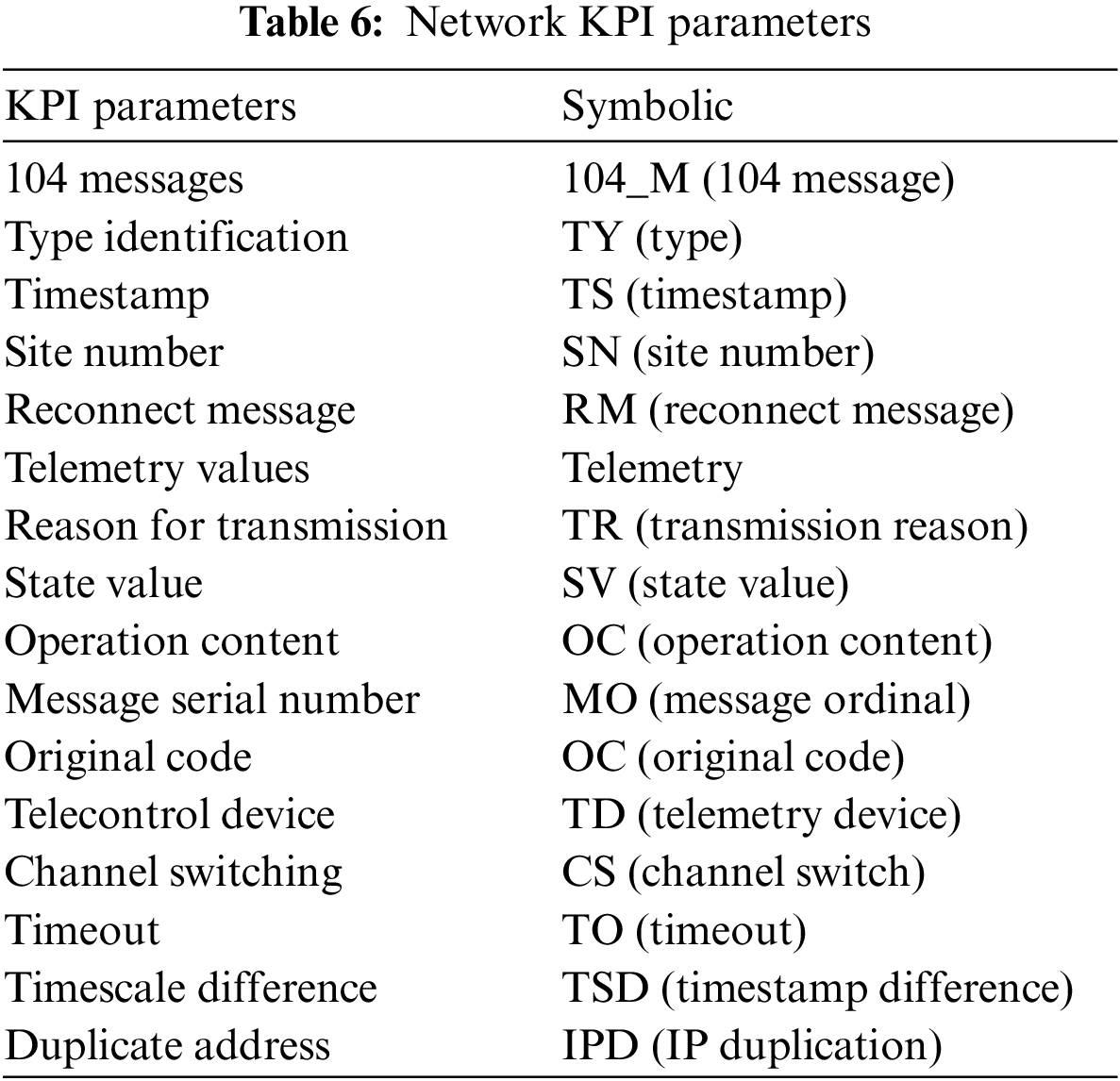
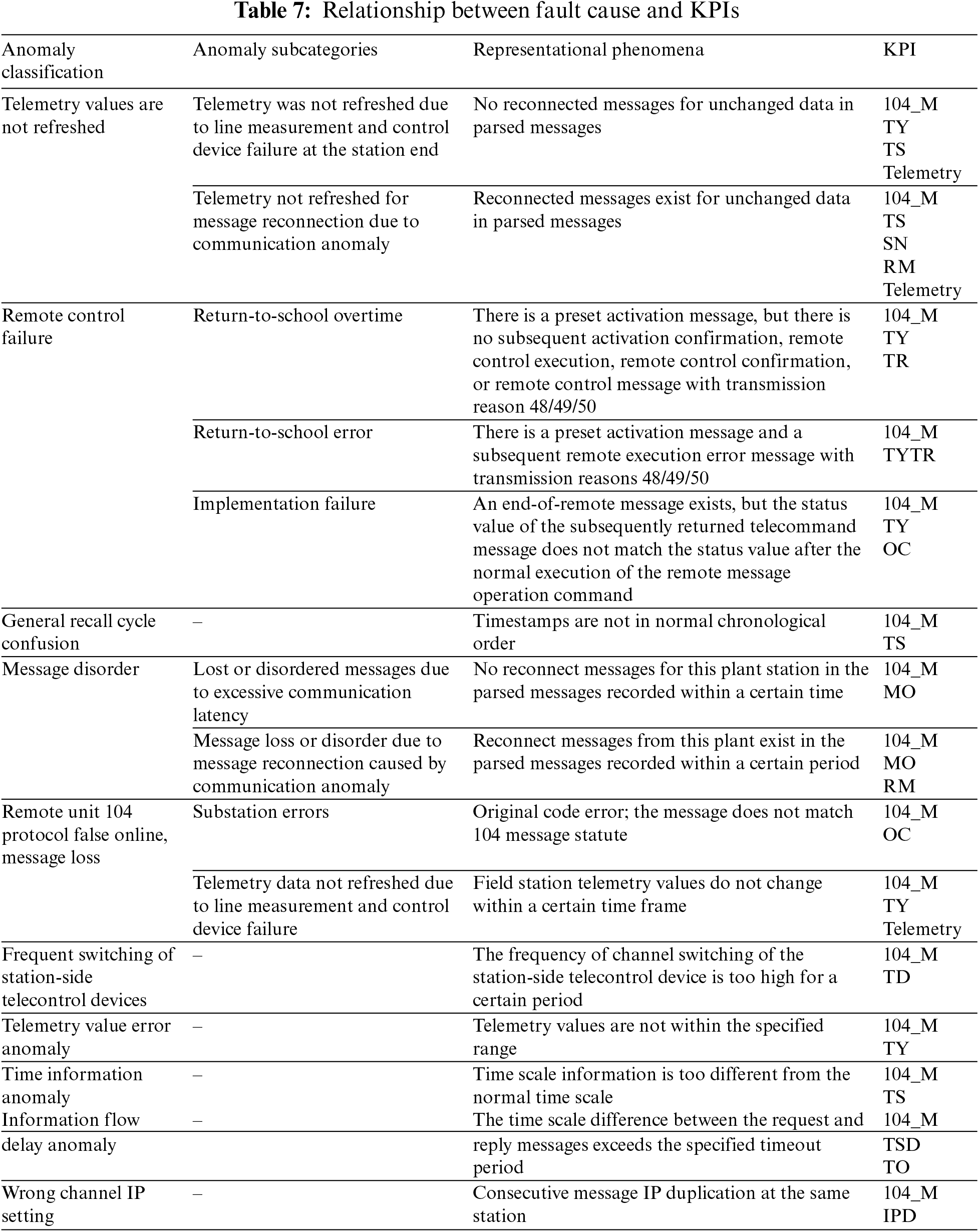
The network failure problem is first analyzed based on the specific network scenario. The most serious fault for operators is a service interruption since this can directly affect user experience and satisfaction. The causes of service interruptions in small areas are mainly linked to five types of faults: uplink interference, downlink interference, coverage voids, nulling faults, and base station faults. A mapping relationship between faults and symptoms was established to filter out useful network parameters (check Tables 6 and 7 at the supplementary files).

4  System Fault Diagnosis and Prediction Based on GANs and Machine Learning

Considering the characteristics of power big data with sequence, timing, and large number, the very small number of abnormal samples, and anomalies including smaller abnormalities, we first use GAN to expand the number of effective samples, then propose a two-step detection algorithm to identify the types of faults (see Fig. 4). In this two-step detection algorithm, XGBoost is used for identify the coarse types of fault (see Fig. 5), and then CNN+LSTM is used for fine-grained analysis to detect the small class of anomalies, where CNN can automatically extract features from massive data and LSTM can handle time series variations to combine the two algorithmic models to better handle various grid anomalies.

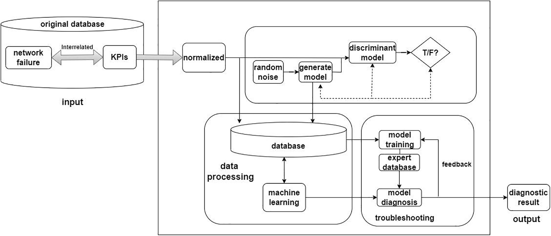
Figure 4: Grid fault detection and diagnosis model based on GANs

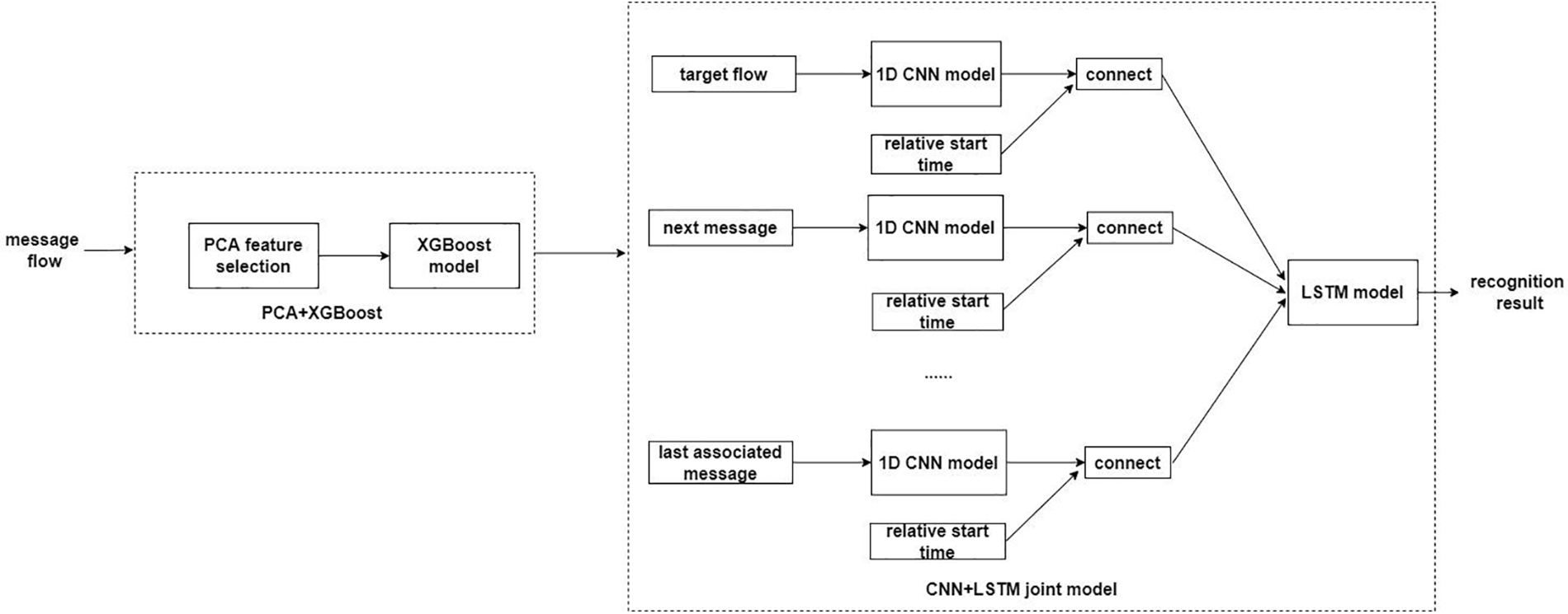
Figure 5: Two-step detection

4.1 Dataset Introduction

The dataset used in this paper is the power grid data obtained from Nanjing Power Supply Company of State Grid Jiangsu Electric Power Co., Ltd. (China) from 2021 to 2022. There are a total of 15 million pieces of data, with a total of 4258 pieces of various fault data. Abnormal data includes telemetry values are not refreshed, remote control failure (return-to-school overtime), remote control failure (return-to-school error), remote control failure (implementation failure), general recall cycle confusion, and message disorder. The original dataset format is in pcap format, which mainly contains the header information of each layer protocol and the 104 protocol message information defined by the power grid. The header information of each layer protocol includes characteristics such as MAC source address, MAC destination address, IP source address, IP destination address, source port number, destination port number, packet size, etc. The 104 message information includes starting characters, APDU length, ISU identification, type identification, and other characteristics.However, the header information of each layer protocol has little help in anomaly identification, so we removed the header information of each layer protocol and only retained the information of protocol 104. In the preprocessing stage of the dataset, we need to process and convert the original dataset into the format read by the model. This process mainly includes the parsing of the original data, truncation and supplementation, decimal conversion, normalization, and annotation of business labels. Among them, parsing raw data involves dividing the collected raw data into four layers based on TCP/IP, including Ethernet layer, IP layer, TCP layer, and 104 packet layer; Truncating and supplementing is to unify the number of bytes in the data packet, truncate the excess parts, otherwise use −9999 as the filling value; Decimal conversion is the process of converting hexadecimal to decimal, which facilitates data processing. Normalization refers to scaling data into a unified space in the same proportion, such as [−1, 1]. The annotation of business labels is to label samples according to the corresponding labels of different types of datasets. Below are two examples of the discrimination between anomalies and normal data:

104 Message data of Telemetry values are not refreshed

[Tue Dec 14 08:19:40 2021]: Z06810D6C51E0A 09 01 03000100 914000340800

[Tue Dec 14 08:19:46 2021]: 680401001E0A

[Tue Dec 14 08:19:47 2021]: 68040100D8C5

[Tue Dec 14 08:19:50 2021]: Z06810D8C51E0A 09 01 03000100 914000340800

[Tue Dec 14 08:19:51 2021]: Z06810DAC51E0A 09 01 03000100 914000340800

From the above five message data, we can see that there exists three continuous message having the same telemetry value 3408. Thus, we can assure that Telemetry values are not refreshed anomaly has occured.

104 Message data of General recall cycle confusion

[Wed Sep 14 00:18:24 2022]: 680E8C234CC0 64 01 06000100 000000 14

[Wed Sep 14 00:18:26 2022]: 680E56C08E23 64 01 07000100 000000 14

[Wed Sep 14 00:18:29 2022]: 680E6AC08E23 64 01 0A000100 000000 14

[Wed Sep 14 01:18:25 2022]: 680E9223F203 64 01 06000100 000000 14

[Wed Sep 14 01:18:27 2022]: 680E02049423 64 01 07000100 000000 14

From the above five message data, we can see that there exists sequential confusion from the timestamp of the third message. Thus, we can assure that General ecall cycle confusion has occured.

4.2 Input Phase

Since different network states have different characteristics, network fault diagnosis and prediction models must know which symptoms correspond to certain network states to identify multiple faults. In this paper, we define S=[KPI1,KPI2,KPI3…,KPIm], which is a vector containing m KPIs as an input vector to characterize different network states. C={FC1,FC2,FC3…,FCn} represents the state of the network (e.g., the network is working normally or has a fault).

The input data vector—consisting of a small sample of data collected from a heterogeneous wireless network environment—is composed of all relevant KPIs for the cell under study. Depending on the granularity required for the diagnostic process, different levels of temporal aggregation (hourly, daily, weekly, monthly, etc.) can be used to collect these KPIs.

If a network fault FCi occurs at T a certain time, then the network status for that time is represented as follows:

SFCi=[KPI1t−T+1KPI2t−T+1⋯KPImt−T+1KPI1t−T+2KPI2t−T+2⋯KPImt−T+2⋮⋮⋱⋮KPI1tKPI2t⋯KPImt](1)

where KPImt refers to the value of the m key performance indicator KPI at the time t.

At the input stage, a specific KPIi is selected and normalized. To ensure that their dynamic ranges are similar and in this system, each key performance indicator KPI is separately normalized based on the maximum value.

KPIi=KPIimax(KPIi)(2)

where KPIi refers to the normalized first key performance indicator and max(KPIi) refers to the first maximum value of the occurrence of the first key performance indicator. This method is used to transform the dynamic range of a specific indicator KPIi to ensure that all variables are within the desired interval. This method only considers values that are not in the interval [0, 1] KPIi.

The normalized network state is represented as follows:

S^FCi=[KPI^1t−T+1KPI^2t−T+1⋯KPI^mt−T+1KPI^1t−T+2KPI^2t−T+2⋯KPI^mt−T+2⋮⋮⋱⋮KPI^1tKPI^2t⋯KPI^mt](3)

4.3 Features Selection

Different exception has different features contributing to the anamoly discrimination.For example, the definition of the telemetry value not refreshing anomaly is that within a certain period of time, the telemetry value of the 104 message with the same station and telemetry value does not change in three consecutive messages. Therefore, it is necessary to judge based on the starting character, type flag, station number, telemetry value, and timestamp of the 104 message. Message disorder exception needs to be determined based on whether the message sequence number is continuous. General recall cycle confusion anomaly needs to be determined based on whether the timestamp order of the message is correct. Similarly, other anomalies can be judged based on the corresponding features of the 104 message, so these features need to be selected as input features for XGBoost. However, CNN+LSTM needs to consider the pre and post message relationship based on the input characteristics of XGBoost, so an additional relative time with the target stream needs to be added.

4.4 GANs

The GAN framework is shown in Fig. 6. It is mainly based on the zero-sum game in game theory, which must have two competing networks that then optimize their objectives simultaneously. The first network, called generator G, outputs simulated samples based on Gaussian noise or uniform noise. The second network, called the discriminator D, feeds samples from the true distribution or samples generated by the generator network G to the discriminator D. The network attempts to label a given sample as 0 (sample from the generator distribution) or 1 (sample from the true data distribution). After some iterations, this competition will make both networks better at the task. In particular, generator G can produce real samples that can fool humans. The objective function of the optimization is

minGmaxDV(D,G)=ES^:pr[logD(S^)]+Ez∼pg[log(1−D(G(Z)))](4)

where pr represents the distribution of the normalized real data s^ collected by the heterogeneous wireless network, pg represents the distribution obeyed by the input noise, and G(Z) is used to represent the mapping of the data space, where G is a differentiable function represented by a multilayer perceptron D(s^). What is obtained is a scalar representing the probability that s^ comes from the real data distribution and not pg.

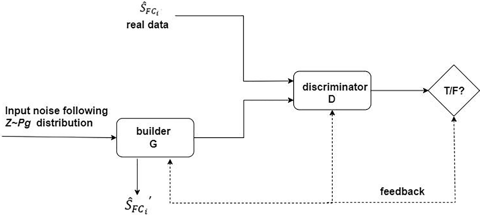
Figure 6: Framework for GANs

As a generative model in the GAN, G does not require a very strict expression for the generated data (as traditional models do), which also avoids incomputability problems when the data are very complex. Also, it does not need to perform some massive computational summatio. It only requires an input of noise that obeys a certain law, a bunch of real data, and two networks that can approximate the function. Through a constant game between the generator and the discriminator, when the discriminator converges to stability, different network states converging to the real data distribution are obtained through the generator S^FCi′.

S^FCi′=[KPI^1t−T+1′KPI^2t−T+1′⋯KPI^mt−T+1′KPI^1t−T+2′KPI^2t−T+2′⋯KPI^mt−T+2′⋮⋮⋱⋮KPI^1t′KPI^2t′⋯KPI^mt′](5)

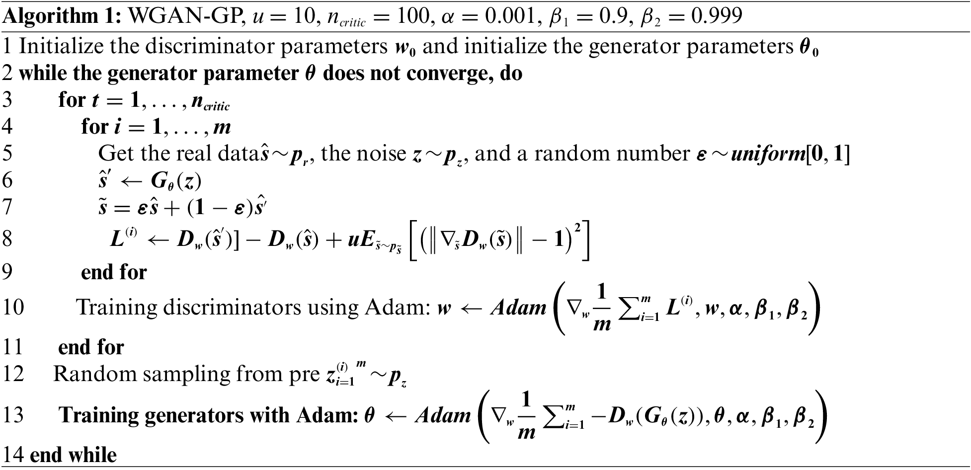
A classical GAN algorithm minimizes the JS scatter between the true and approximate distributions. However, the JS metric is not continuous, and this gradient is not available in some places. To overcome this drawback, Goodfellow et al. [19] proposed replacing the JS metric with the Wasserstein distance, while WGAN guarantees the availability of the gradient in all places. Given that the Wasserstein distance equation is very difficult to solve, WGAN uses Kantorovich-Rubinstein duality to simplify the computation while introducing a fundamental constraint for the discriminator to find the 1-Lipschitz function. The weights of the discriminator are trimmed to satisfy the constraint within a certain range of hyperparameter control. The WGAN algorithm with a gradient penalty (hereafter referred to as WGAN-GP) uses a gradient penalty to enforce the 1-Lipschitz constraint rather than weight clipping. In this paper, WGAN-GP is used to generate simulation data. The optimization objectives are as follows.

L=Es^′∼pg[D(s^′)]−Es^∼pr[D(s^)]+uEs~∼ps~[(‖∇s~Dw(s~)‖−1)2](6)

where s^′∼pg represents the distribution obeyed by the data generated by the generator and s^∼pr is the distribution obeyed by the real data, which in this case refers to the distribution of the normalized small sample data collected under different network states in a heterogeneous wireless network environment. s~ is obtained by performing sampling on the whole data set consisting of real and generated data. In this paper, we use ε∼uniform[0,1] and then randomly interpolate the sampling on the concatenation of s^′ and s^ to obtain s~=εs^+(1−ε)s^′. Es~∼ps~[(‖∇s~Dw(s~)‖−1)2] is a penalty term. The closer ‖∇s~Dw(s~)‖2 is to 1 in the penalty term, the less penalty is expected, while u is the penalty parameter. The specific implementation process of WGAN-GP is presented in Algorithm 1. The number of discriminant iterations at the fixed generator is ncritic and the batch size is m. The hyperparameters of Adam’s algorithm for discriminator as well as generator training are defined as follows: α is the learning rate (used to control the step size), β1 is the exponential decay rate of the first-order moment estimation, and β2 is the exponential decay rate of the second-order moment estimation.

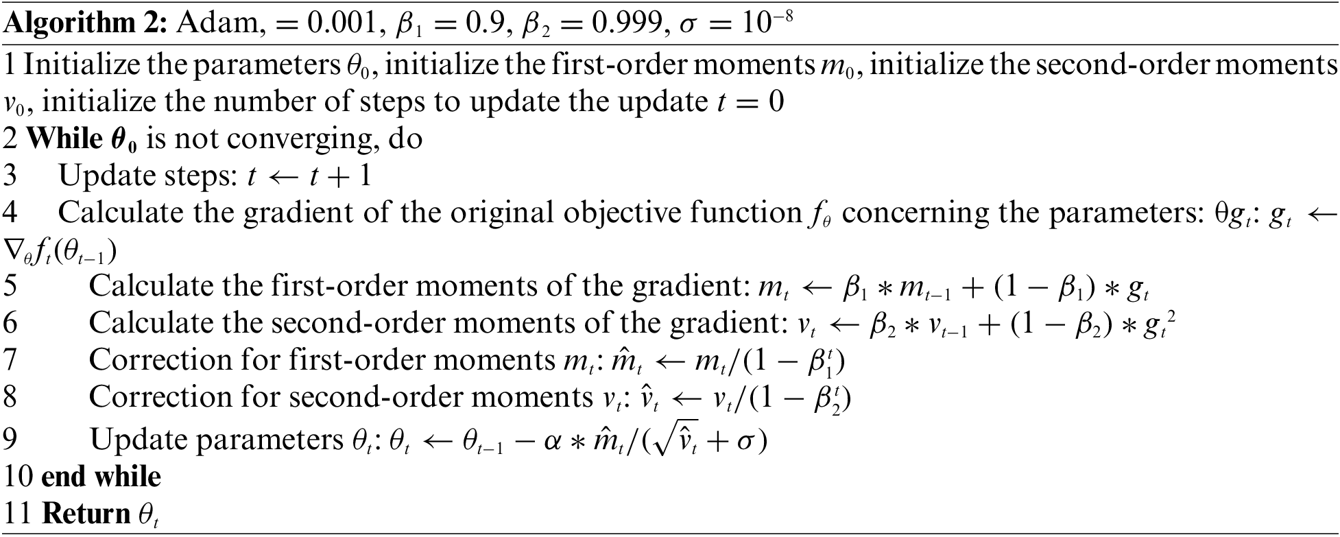
For the training of the discriminator and the generator, this study uses the adaptive moment estimation (Adam) algorithm for parameter updating, which is defined as follows: t, the number of steps to update; α, the learning rate, used to control the step size; θ, the parameters required to update; fθ, the stochastic objective function with parameters θ, generally referred to as the loss function; gt, the gradient obtained by deriving the objective function fθ; β1, the exponential decay rate of the first-order moment estimate; β2, the exponential decay rate of the second-order moment estimate; mt, the first-order moment of the gradient gt, the expectation of the gradient gt; vt, the second-order moment of the gradient gt, the expectation of the gradient gt2; m^t, the bias correction of mt; v^t, the bias correction of vt.

The main idea of Adam is to use the first-order moment estimation and second-order moment estimation of the gradient to dynamically adjust the learning rate of each parameter to achieve the purpose of parameter updating. The advantage of Adam is that after bias correction, the learning rate of each iteration is fixed in a certain range, making the parameters relatively stable. The specific implementation process of Adam is provided in Algorithm 2.

4.5 XGBoost

Extreme gradient boosting (eXtreme Gradient Boosting, XGBoost) is an improved algorithm based on the gradient boosting decision tree (GBDT) in terms of computational speed, generalization performance, and scalability. The original GBDT algorithm builds a new decision tree model in the direction of gradient descent of the previous model loss function at each iteration during training, pruning it after constructing the decision tree. Unlike the original GBDT, XGBoost adds the regularization term to the loss function during the construction phase of the decision tree. This process can be described by the following equation:

Fobj(m)=∑i=1NL(yi,y^i(m))+Ω(fm)(7)

where L(yi,y^i(m)) is the loss function that measures the difference between the predicted value y^i(m) and the target value yi, which, in the text, means the difference between the predicted network state label and the true network state label.

L(yi,y^i(m))=(yi−y^i(m))2(8)

Ω(fm) is the regularization term, defined as

Ω(fm)=γT+12λ∑j=1Twj2(9)

where T refers to the number of leaf nodes, λ is the regularization parameter, γ is the learning rate, and wj denotes the predicted value of the j leaf node.

Let y^i(m−1) denote the optimal solution to the existing (m−1) tree and the second-order Taylor expansion of the loss function Fobj(m) at y^i(m−1) be

Fobj(m)=∑j=1T[Gjwj+12(Hj+λ)wj2]+γT(10)

where:

Gj=∑i∈Ij∂y^(m−1)L(yi,y^(m−1))(11)

Hj=∑i∈Ij∂2y^(m−1)L(yi,y^(m−1))(12)

Ij is defined as the index set of samples whose values are associated with the leaf node j.

Assuming that the structure of the decision tree has been determined, the predicted value at each leaf node can be obtained by making the derivative of the loss function zero, which can be written as:

wj∗=−GjHj+λ(13)

Substituting the predicted values into the loss function yields the minimum value of the loss function:

Fobj∗=−12∑j=1TGj2Hj+λ+γT(14)

Fobj*Fobj∗ is the final loss function, and the smaller its value, the closer it is to the actual result, indicating a better structure of the tree.

4.6 CNN+LSTM

A CNN is a feed-forward neural network with artificial neurons that respond to a portion of the surrounding units in the coverage area and excels for large image processing. A CNN consists of one or more convolutional layers and a top fully connected layer (corresponding to a classical neural network), while also including associative weights and a pooling layer. This structure allows CNNs to exploit the 2D structure of the input data. Compared to other deep learning structures, CNNs can give better results in fields like image recognition [26]. This model can also be trained using a backpropagation algorithm. Compared to other deep feed-forward neural networks, CNNs require fewer parameters to be considered, which has resulted in the CNN being a widely used deep learning structure.

An LSTM is a special type of recurrent neural network (RNN), while an RNN is a type of neural network used for processing temporal data, compared to the general neural network, it can handle sequence-changing data [27]. Moreover, LSTM is mainly designed to solve the gradient disappearance and gradient explosion problems during the training of long sequences. Simply, this means that an LSTM can have better performance in longer sequences when compared to an ordinary RNN. Thus, for temporal features, LSTM can be used to identify them and CNN can handle data with massive variable features. For message feature issues, CNN can be used to identify them, while the combination of the two (i.e., LSTM+CNN) can handle a variety of anomalous grid features.

In this paper, we use the XGBoost and CNN+LSTM frameworks to train the data and then use the trained model to predict the state of the network at a certain period (i.e., to label the otherwise unknown data collected). In addition, another benefit of using XGBoost is that an importance score can be obtained for each attribute after a boosted tree has been created. In general, the importance score measures the value of an attribute in the model to enhance the construction of the decision tree. The more an attribute is used in the model to build a decision tree, the more important it is. Therefore, in this study, we also used the feature importance ranking function of the XGBoost framework to preprocess the data and select the most relevant performance metrics that affect the measurement of the network state. Using this algorithm, a trade-off can be made between the accuracy of the test set and the complexity of the model. Moreover, considering the characteristics of the grid anomaly data, the XGBoost-processed data is further fed into the joint CNN+LSTM model for fine-grained analysis to achieve the efficient and reliable detection of grid faults.

4.7 Parameters Settings

The default parameters are used for GAN, SVM, CNN, KNN, RT, and XGBoost. The WGAN-GP parameter settings are shown in Section 4.2. The CNN+LSTM model construction includes convolutional layer, pooling layer, LSTM layer, and fully connected layer. In training model stage, Firstly, construct a CNN convolutional neural network. The CNN neural network model of this system uses a one-dimensional CNN based model, which includes four convolutional layers, two maximum pooling layers, two LSTM layers, and two fully connected layers. The number of neurons in Conv1 and Conv2 is 256, the size of the kernel is 3, and the step size of all zeros filling is 1; The number of neurons in Conv3 and Conv4 is 128, with a kernel size of 2 and a zero fill step size of 1; The kernels of the two maximum pooling layers are 2, with a zero fill step size of 2; Two LSTM layers are connected in parallel with CNN, with 128 and 256 neurons respectively and 64 input data sizes. The number of neurons in two fully connected layers is 128. Each pool layer uses batch normalization. The activation function used by the four convolution layers is ReLU function. The Adam optimization algorithm of the training model is the maximum 30 epochs, and the learning rate is 0.001. The network uses early stop, that is, when the training is within 5 epochs, the loss function does not improve, then the training is terminated. After the business recognition model is constructed, the divided training set is input to automatically extract features, and the model is trained based on the extracted features, continuously adjusting model parameters to generate a business recognition model. Save the trained initial model. At this stage, the number of layers of CNN, the connection order of convolution layer and pooling layer, the size and number of convolution cores, and the selection of activation function will all affect the training effect of the model.

5  Performance Analysis

In this paper, the data set is from the power grid of Nanjing Power Supply Branch of Jiangsu Electric Power Co., Ltd. (China). From year 2021 to 2022. There are a total of 15 million pieces of data, and a total of 4258 pieces of various fault data. For abnormal data, the original PCAP data packet is screened out to only contain 104 message information, and the TCP information in front of the 104 data is removed, and only the ASDU part of the 104 message is retained. According to the meaning represented by each byte of the 104 message, it is then converted into CSV format as input data, and the specific exception classification is introduced in Section 4.

To demonstrate the performance of the identification methods, this study involved conducting various comparative experiments on massive data anomaly identification methods for dispatch automation systems based on the combination of GANs and machine learning. This includes GAN parameter selection, the performance analysis of various algorithms, and the comparison of two-step anomaly detection methods with individual algorithms.

5.1 GAN Parameter Selection

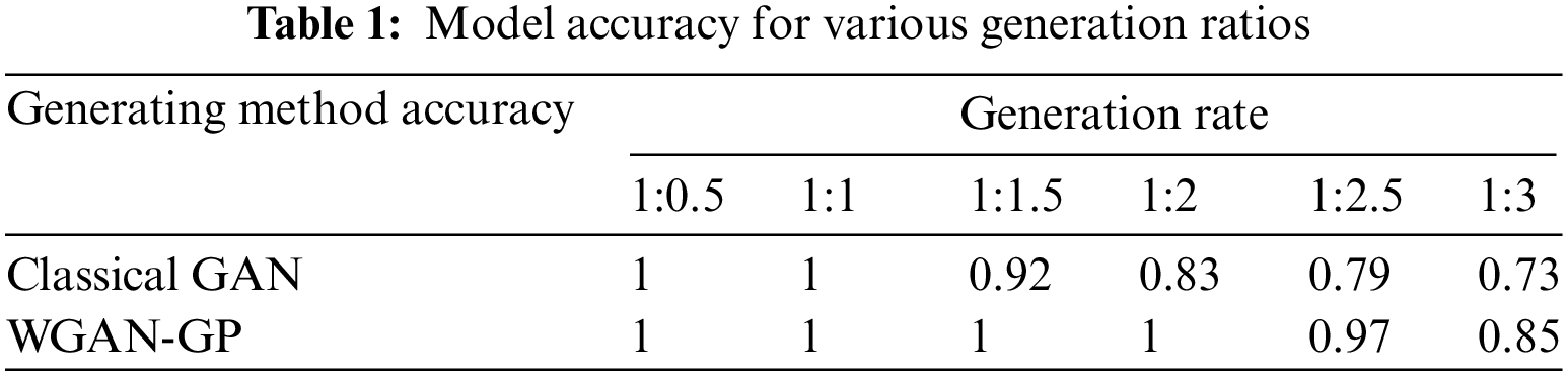
For the generation samples, we compared and analyzed two algorithms—classical GAN and WGAN-GP—thus selecting the best generation samples and testing the best generation sample ratio.

Two testing methods are established in this paper. One is to test the generated samples against the model trained with the original data (generated data accuracy), while the other is to test the generated samples against the original data by training the model with the generated samples (generated model accuracy). The samples generated by the two algorithms are compared. The test set for testing the generative model accuracy is the same as the original data set required to generate the samples, while the original model for testing the generative data accuracy is the same as the original data set required to generate the samples. For example, the number of raw samples for telemetry value non-refreshing anomalies is 1069.

The accuracy of the generated data was first tested. These results are presented in Table 1. From Table 1, it can be seen that the optimal generation ratio of WGAN-GP is much larger than that of the classical GAN generation algorithm.

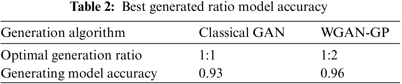
Next, the accuracy of the generated models was tested. The data generated by selecting the best generation ratio of each algorithm was input to the XGBoost algorithm for training to get the model, and the generated model was tested with the same original anomaly samples shown in Table 2. In Table 2, it can be seen that the accuracy of the generated model of WGAN-GP is slightly higher than that of the classical GAN generation algorithm. Based on comprehensive consideration, the WGAN-GP algorithm was chosen to expand the samples.

5.2 Algorithm Performance Analysis

Since some of the algorithms have a demand on the number of datasets, we selected three anomalies with a large number of datasets from a variety of anomalies: telemetry not refreshed, total call cycle confusion, and message disorder. The test set accuracies are presented in Table 3.

From Table 3, we can see that both the XGBoost and CNN+LSTM models have high recognition accuracy for all anomalies, while CNN+LSTM has higher sensitivity to temporal anomalies such as total call cycle chaos. Therefore, in the next two-step anomaly detection method, the first step uses XGBoost to analyze the large class of anomalies, while the second step of fine-grained anomaly detection then inputs the recognition results of the first step into the joint CNN+LSTM model to output the results.

5.3 Two-Step Anomaly Detection Method

To demonstrate the superiority of the two-step detection method, we compared the two-step detection method with several algorithms in terms of test accuracy. The algorithms used for comparison include XGBoost and CNN+LSTM (see Table 4). Taking the exception of remote control failure as an example, the major category of remote control failure anomalies can be subdivided into three subcategories based on more detailed fault causes: return-to-school timeout, return-to-school error, and execution failure. Notably, both are data sets augmented by the WGAN-GP generation method. The results are presented in Table 4.

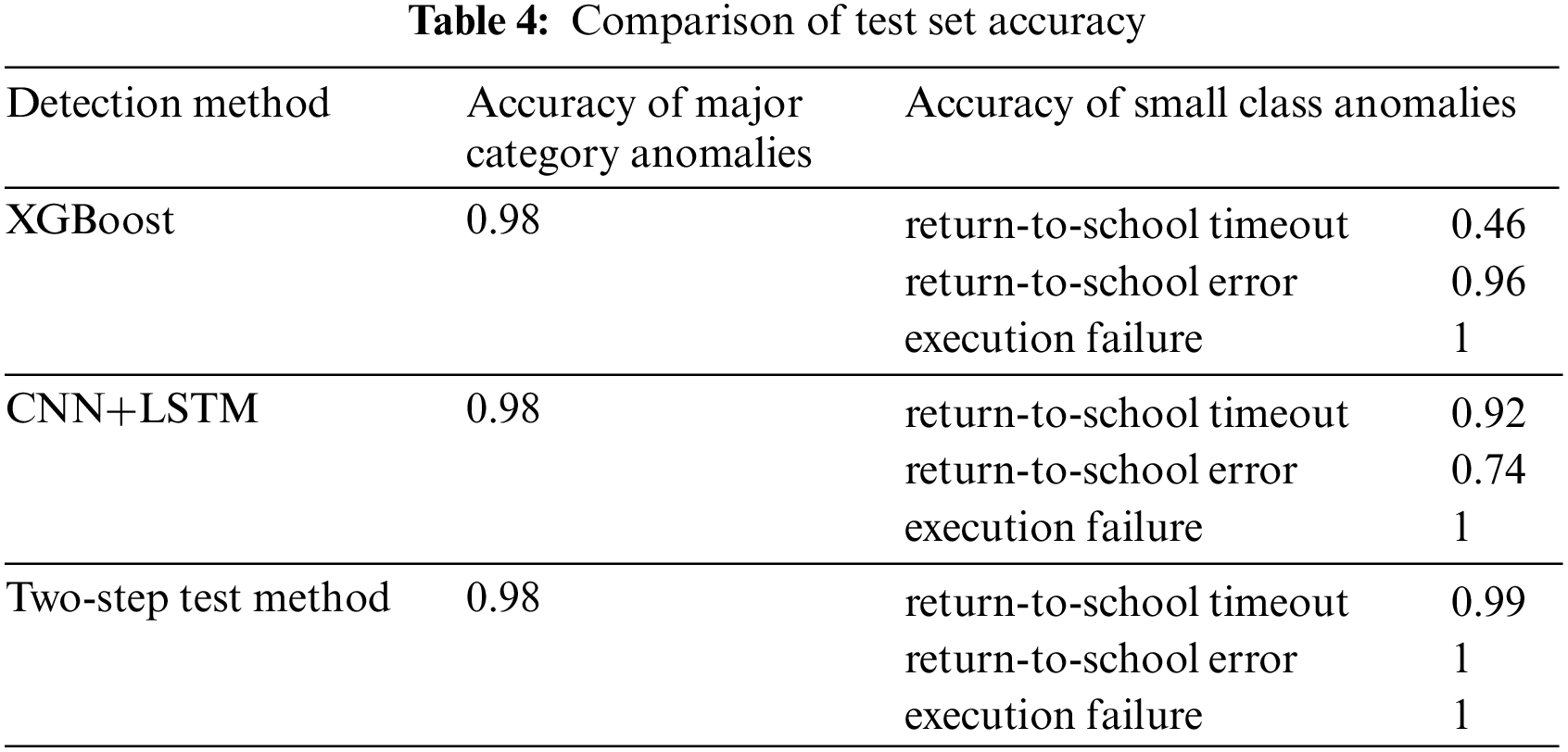
It can be seen from Table 4 that for the detection of large categories of anomalies, the accuracy rates of the three methods are the same. However, for the detection of small class anomalies, the accuracy rate of using only XGBoost algorithm or CNN+LSTM algorithm is lower than that of the two-step detection method, so the two-step detection method can effectively improve the identification accuracy of small class anomalies.

5.4 Comparison of Classification Accuracy before and after Sample Expansion

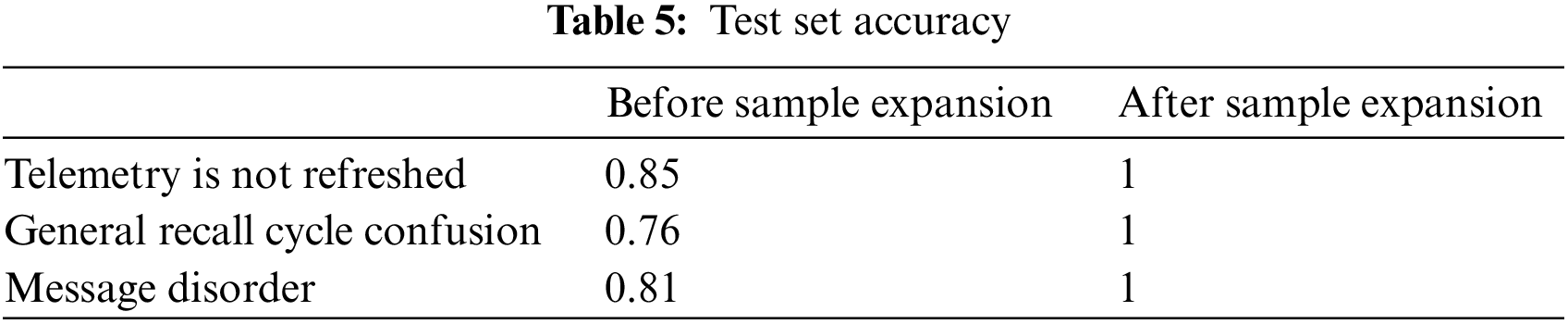
It can be seen from Sections 4.1–4.3 that after many experiments and evaluation, we have determined that the sample generation algorithm is WGAN-GP and the anomaly identification algorithm is a two-step detection algorithm, that is, first use XGBoost to test large class anomalies and then use CNN+LSTM to detect small class anomalies, in order to further prove that the method proposed in this paper can achieve efficient and reliable power grid fault diagnosis. We compared the accuracy of various anomalies before and after sample expansion. This section uses a two-step detection algorithm and selects three common anomalies for comparison, namely, Telemetry values that are not refreshed, General recall cycle confusion, and Message disorder. Before expansion, the number of three types of anomalies samples is 1635, 397, and 2006, respectively. The WGAN-GP algorithm is used to expand the original sample to the expanded sample ratio of 1:2. The test set is the original sample, and the number is 100. The comparison results are shown in the following table. It can be clearly seen from the Table 5 that after the expansion of WGAN-GP samples, the recognition accuracy has been greatly improved, with an increase of 15%–24%. Therefore, after expanding the samples based on WGAN-GP algorithm, the two-step detection algorithm proposed in this paper can achieve efficient and reliable power grid fault diagnosis, effectively solving the problems of insufficient experimental training mark samples and low recognition accuracy.

6  Conclusion

In this paper, we propose an anomaly identification, diagnosis and prediction method based on GAN and two-step detection method for massive data flow of dispatching automation system according to the characteristics of abnormal data in power grid. First of all, WGAN-GP is used to generate a large number of reliable data that match the characteristics of power grid anomaly data, which solves the problem of insufficient labeled data set in machine learning. Secondly, a two-step detection method is designed. First, XGBoost is used to detect large-category anomalies, and then CNN+LSTM is used to detect small-category anomalies, which solves the problem of low accuracy of traditional machine learning in identifying power grid anomalies. The experimental results show that the algorithm proposed in this paper can achieve efficient and reliable power grid fault diagnosis. However, this paper mainly focuses on identifying known anomalies in the power grid. There are still many unknown anomalies waiting for us to discover, so we will further explore the possible unknown anomalies in the power grid with the help of unsupervised learning.

Funding Statement: This work was supported by the Technology Project of State Grid Jiangsu Electric Power Co., Ltd., China, under Grant J2021167.

Conflicts of Interest: The authors declare that they have no conflicts of interest to report regarding the present study.

References

1. X. Xu, “Game theory for distributed IoV task offloading with fuzzy neural network in edge computing,” IEEE Transactions on Fuzzy Systems, vol. 30, no. 11, pp. 4593–4604, 2022. [Google Scholar]

2. F. H. Ying, N. Z. Xu and Y. T. Ji, “Anomaly detection of power data network service flow based on KTLAD,” Journal of Beijing University of Posts and Telecommunications, vol. 31, no. 16, pp. 108–111, 2017. [Google Scholar]

3. H. J. Wang, Z. Q. Li, H. Zhao and Y. J. Yue, “Research on abnormal power consumption detection based on SVM in AMI environment,” Electrical Measurement and Instrumentation, vol. 26, no. 21, pp. 64–69, 2014. [Google Scholar]

4. Y. P. Yang and Z. H. Xu, “Application research of outlier detection method based on cluster analysis in power grid data quality management,” Modern Electronic Technology, vol. 28, no. 15, pp. 137–139, 2016. [Google Scholar]

5. Z. Pang, M. N. Li and J. D. Li, “ANOMALOUS: A joint modeling approach for anomaly detection on attributed networks,” in Twenty-Seventh Int. Joint Conf. on Artificial Intelligence (IJCAI-18), vol. 33, no. 25, pp. 3513–3519, 2018. [Google Scholar]

6. Y. Xu, S. A. Li and Y. H. Huang, “Detection of abnormal power consumption behavior of users based on CNN-GS-SVM,” Control Engineering, vol. 28, no. 16, pp. 1989–1997, 2021. [Google Scholar]

7. Z. D. Yang, J. W. Dong, G. J. Cai, X. J. Kai and M. Sha, “Research on abnormal electricity consumption detection method based on LightGBM and LSTM model,” Electrical Measurement and Instrumentation, vol. 28, no. 17, pp. 1738–1749, 2022. [Google Scholar]

8. D. Li, Z. W. Jiang, Y. W. Zeng, Y. Q. Huang and Y. W. Xu, “LDSAD-based network traffic anomaly detection in power monitoring system,” Zhejiang Electric Power, vol. 21, no. 33, pp. 87–92, 2022. [Google Scholar]

9. S. Ul Amin, M. Ullah, M. Sajjad, F. Alaya Cheikh, M. Hijji et al., “EADN: An efficient deep learning model for anomaly detection in videos,” Mathematics, vol. 24, no. 18, pp. 243–257, 2022. [Google Scholar]

10. Y. J. Yang, G. M. Sha and Y. F. Cai, “Anomaly detection method for status data of power transmission and transformation equipment based on big data analysis,” Chinese Journal of Electrical Engineering, vol. 21, no. 19, pp. 53–59, 2015. [Google Scholar]

11. T. Pei and D. L. Qin, “Power data anomaly detection method based on time series extraction and Voronoi diagram,” Electric Power Construction, vol. 31, no. 24, pp. 105–110, 2017. [Google Scholar]

12. Y. Wang, L. Dong and X. Z. Huang, “Detection method for weighted power line stealing electricity based on analytic hierarchy process,” Science Technology and Engineering, vol. 27, no. 17, pp. 96–103, 2017. [Google Scholar]

13. D. W. Pan, D. D. Li and J. Zhang, “Anomaly detection for satellite power subsystem with associated rules based on kernel principal component analysis,” Microelectronics Reliability, vol. 55, no. 3, pp. 2082–2086, 2015. [Google Scholar]

14. X. Xu, T. Huang, Z. Xu, Q. Li, H. Qin et al., “DisCOV: Distributed COVID-19 detection on X-Ray images with edge-cloud collaboration,” in 2022 IEEE World Congress on Services (SERVICES), Barcelona, Spain, pp. 23, 2022. [Google Scholar]

15. Q. Li, L. Wang, Z. Xu, D. Wang, X. Xu et al., “A correlation graph based approach for personalized and compatible web APIs recommendation in mobile App development,” IEEE Transactions on Knowledge and Data Engineering, vol. 35, no. 6, pp. 5444–5457, 2023. [Google Scholar]

16. Z. Xu, L. Wang, L. Wang, Y. Kai and S. Shimizu, “Hierarchical adversarial attacks against graph-neural-network-based IoT network intrusion detection system,” IEEE Internet of Things Journal, vol. 9, no. 12, pp. 9310–9319, 2022. [Google Scholar]

17. L. Zhang, “A knowledge-driven anomaly detection framework for social production system,” IEEE Transactions on Computational Social Systems, vol. 32, no. 21, pp. 1–14, 2022. [Google Scholar]

18. L. Wang, “Intrusion detection for maritime transportation systems with batch federated aggregation,” IEEE Transactions on Intelligent Transportation Systems, vol. 24, no. 2, pp. 2503–2514, 2023. [Google Scholar]

19. I. Goodfellow, J. Pouget-Abadie, M. Mirza, B. Xu, D. Warde-Farley et al., “Generative adversarial nets,” in Int. Conf. on Neural Information Processing Systems, MIT Press, Cambridge, MA, USA, pp. 2672–2680, 2014. [Google Scholar]

20. M. Arjovsky and L. Bottou, “Towards principled methods for training generative adversarial networks,” arXiv:1701.04862, 2017. [Google Scholar]

21. C. J. Mowlaei, E. M. and X. Shi, “Population-scale genomic data augmentation based on conditional generative adversarial networks,” in Proc. of the 11th ACM Int. Conf. on Bioinformatics, Computational Biology and Health Informatics, New York, NY, USA, pp. 1–6, 2020. [Google Scholar]

22. L. Zhang, “Integrated CNN and federated learning for COVID-19 detection on chest X-ray images,” IEEE/ACM Transactions on Computational Biology and Bioinformatics, vol. 31, no. 23, pp. 1243–1249, 2022. [Google Scholar]

23. Q. Li, Y. Yang, Z. Xu, W. Rafique and J. Ma, “Fast anomaly identification based on multiaspect data streams for intelligent intrusion detection toward secure Industry 4.0,” IEEE Transactions on Industrial Informatics, vol. 18, no. 9, pp. 6503–6511, 2022. [Google Scholar]

24. K. Li, “Time-aware missing healthcare data prediction based on ARIMA model,” IEEE/ACM Transactions on Computational Biology and Bioinformatics, vol. 21, no. 27, pp. 257–273, 2022. [Google Scholar]

25. Z. Xu, X. Xu, L. Wang, Z. Zeng and Y. Zeng, “Deep-learning-enhanced multitarget detection for end-edge–cloud surveillance in smart IoT,” IEEE Internet of Things Journal, vol. 8, no. 16, pp. 12588–12596, 2021. [Google Scholar]

26. L. Huang, G. Xu and D. Samaras, “Wasserstein GAN with quadratic transport cost,” in 2019 IEEE/CVF Int. Conf. on Computer Vision (ICCV), Seoul, Korea (Southpp. 4831–4840, 2019. [Google Scholar]

27. Y. Yang, “ASTREAM: Data-stream-driven scalable anomaly detection with accuracy guarantee in IIoT environment,” IEEE Transactions on Network Science and Engineering, vol. 21, no. 25, pp. 1, 2022. [Google Scholar]

Supplementary Materials

Table 6 is a mapping table of the name of anomalies and their abbreviation. Table 7 gives a clear description of the cause and representative phenomena of the anomalies.