A Nonlinear Spatiotemporal Optimization Method of Hypergraph Convolution Networks for Traffic Prediction

1  Introduction

With the rapid development of information technology, artificial intelligence [1] involves many interdisciplinary subjects such as human–machine interaction [2] and health state estimation [3], and brings new elements to intelligent transportation systems (ITS). Traffic prediction is the cornerstone of ITS [4]. By learning potential traffic information and rules, ITS can predict the traffic states in the future, so as to take appropriate traffic control measures in time. Thus, accurate and reliable prediction plays an important role in practical traffic applications, such as traffic guidance and signal control.

Traditional traffic prediction mainly relies on subjective judgment. The data-driven method [5] relies on direct data analysis, and offers higher accuracy in the fields of intelligent recommendation [6,7], behavioral analysis [8] and blockchains [9]. It is found that the potential spatiotemporal evolution rules and characteristics of traffic states from massive data, which have become the mainstream for traffic state analysis [10,11]. Traffic data is critical for accurate traffic prediction [12]. It is a spatiotemporal dataset with spatial structure differences and dynamic changes over time. Temporally, traffic data of all nodes on the road network structure can be regarded as a time series, the observed value of each node is obviously correlated with that of its adjacent time steps [13–15]. Spatially, the traffic states of a certain road segment are correlated with the nearby locations or the relevant areas [16,17]. The prediction models that only consider the influence of historical data or adjacent road segments are not fully applicable to spatiotemporal traffic data. Nowadays, the models have evolved to the spatiotemporal dimensions.

Deep learning models have been extensively applied in traffic prediction [18]. As an important part, the graph learning methods [19,20] utilize the graph structure and the corresponding node features to learn the internal geometric relations of the structural data, by mapping the features of the graph to the feature vectors with the same dimension in the embedding spaces. To utilize such spatial features, it’s appropriate to formulate traffic networks as graphs [21]. They can not only retain the original structural information and multi-dimensional features of traffic data, but also show strong expressive ability and self-training performance. Recently, traffic prediction utilizes graph learning models, which have a good interpretation for the model results [22–24].

Despite the empirical success of the aforementioned techniques, two issues in traffic prediction enabled by graph learning still exist: 1) Traffic prediction is a complex process, the nonlinear optimization parameters of multiple dependencies cannot be determined, which limits the models to capture the spatiotemporal evolution characteristics of traffic states [25]; 2) It fails to consider the higher-order relationship between spatial structures, and integrate these associated data uniformly.

Hypergraph convolutional networks (HGCN) [4] have a strong ability of higher-order spatial representation in information transfer between graph structures. Additionally, extended Kalman filter (EKF) can approximate linearize the nonlinear state-space model, and utilize the model parameters to estimate the spatiotemporal states, which are suitable for estimating the complex traffic states in road networks [26,27]. Motivated by this, a nonlinear spatiotemporal optimization method of hypergraph convolution networks (HGC-NOM) is proposed. The method utilizes the higher-order spatial features of the road network captured by HGCN, and dynamically integrates them with the historical data to weigh the influence of spatiotemporal dependencies. On this basis, EKF is used to improve the accuracy of online traffic prediction. The major contributions of this work can be summarized as follows:

(1) To optimize these nonlinear parameters of multiple dependencies in the process of spatiotemporal fusion, the proposed method utilizes recursive least squares (RLS) to identify the dynamic weights of the factors of the higher-order spatial features and the historical data, and utilizes EKF to online update the state vector-values reflecting the actual traffic environment, so as to improve the generalization ability and prediction accuracy.

(2) In view of the lack of considering correlated spatial characteristics of non-adjacent road segments, the higher-order spatial feature extraction model based on HGCN is presented. The hypergraph structures are constructed by connecting non-adjacent road segments with hyperedges. On this basis, the Laplacian matrix on the hypergraph is defined, and HGCN utilizes Chebyshev polynomials to capture the implicit spatial features of different segments.

(3) Extensive experiments were confirmed the validity of the proposed method and the characteristic contribution of spatiotemporal fusion factors. The experimental results show that the performance of the proposed method is superior to that of the state-of-the-art methods.

The rest of the work is organized as follows: Section 2 describes the state-of-the-art methods. In Section 3, the model of HGCN is introduced. Section 4 explains the proposed method in detail. Section 5 illustrates the experimental results and discusses the feasibility. Finally, Section 6 concludes the work.

2  Related Work

Traffic prediction is the key to the realization of traffic control and guidance, and it is the premise to reduce traffic congestion and improve travel efficiency. With the rapid development of information technology, traffic spatiotemporal data is increasingly abundant. The models gradually evolve from historical statistical methods to the deep learning methods [28–30] based on spatiotemporal fusion.

Historical statistical methods mainly used the significant temporal relationship between historical data, as well as traffic flow, average speed and other parameters to make prediction. Jing et al. [31] assessed the multistep speed predictive performance of eight different models using 2-min road segment speed data collected from remote traffic microwave sensors. Kong et al. [32] utilized particle swarm optimization algorithm to calculate traffic parameters from the aspects of accuracy, immediacy and stability, and applied the fuzzy classification method to convert the predicted parameters into the congestion states recognized by residents. Liu et al. [33] integrated the traffic features extracted and the measured values of microwave sensors for state estimation, proposed a combination method of state-space model and EKF, and adaptively predicted the changes of traffic conditions. Considering the complexity of traffic conditions, Zhu et al. [34] identified the fitted historical data, weather, date attributes and other influencing factors by recursive least square parameters, and used EKF to predict the average speed. All above methods failed to consider spatial dependency, thereby limiting their ability to capture the traffic state governed by the road network structures.

The prediction model [35] based on deep learning will reflect the adaptability of data state through sample training, so as to capture the nonlinear features between different variables. Combining the acceleration of the target segments and the speed of the adjacent segments, Ye et al. [36] utilized the optimized neural network to improve the predictive performance, but the phase transition theory was needed for further improvement. Tang et al. [37] used K-means algorithm to divide the speed samples into different clusters, measured the membership degree of the samples, and established the fuzzy neural network rules to predict the traveling speed. Zhang et al. [38] constructed a multi-task learning model based on deep learning, selected the information of each link through the nonlinear causality detection method, adjusted the model parameters and optimized the traffic predictive performance. Traffic prediction is not only closely related to traffic conditions based on temporal dimension, but also affected by traffic conditions of other spatial locations, such as upstream and downstream locations, and adjacent lanes. Zhang et al. [39] constructed a residual neural network framework in traffic networks, adopted a deep learning method to dynamically aggregate spatiotemporal values and predicted the traffic flow in each region. Wu et al. [40] proposed a cross-city spatiotemporal migration learning model, obtained prior knowledge by training the traffic data of source cities, and designed a learning strategy based on generative adversarial network to improve the predictive performance. The structures of traffic networks present non-Euclidean rules [41], so these methods were limited to European structural data such as convolutional neural networks [42,43], which had difficulties in the spatial modeling of traffic networks.

Graph learning methods extract the feature information of adjacent segments, and transform the non-European road network structures [44]. Based on these characteristics, it is appropriate to formulate road networks as graphs [21]. Some scholars began to explore the spatiotemporal prediction combining deep learning [45] and graph theory. Yu et al. [22] constructed a deep learning framework based on graph convolutional network (GCN) to capture the spatiotemporal correlation of multi-scale traffic networks, and satisfied the requirements of mid-and-long term prediction tasks. Due to the prominent effect of the attention mechanism in selecting key information, Guo et al. [23] proposed an attention-based GCN model, weighted fusion of three date attribute components, including recent, daily period and weekly period, and captured the dynamic spatiotemporal correlation to generate prediction results. Yu et al. [46] adopted the spatiotemporal transformer mechanism to capture the spatial interaction of crowds and complex temporal dependence, and proposed a transformer-based GCN model to predict the flow of social crowds in road networks. Combining self-attention mechanism, Ye et al. [24] established transformer model based on meta-graph learning, extracted spatiotemporal heterogeneity in traffic networks, and predicted traffic states by auto-regression. In order to find the constraints of traffic network topology and the rule of dynamic change over time, references [47,48] improved the spatiotemporal dependencies under graph learning framework, which dynamically captured the temporal dependence from the gated recurrent unit and adaptively derived the node attributes of the optimal graph structures, and proved the validity and interpretability of these traffic prediction methods.

To sum up, the existing models are lack of consideration of road network spatial features, and cannot comprehensively analyze the influences of cross-node isomorphism in urban road networks. Graph learning based models depend on the accuracy of the graph structural representation of traffic data with spatial correlations, but ignore the higher-order spatial feature extraction and nonlinear movement of spatiotemporal prediction. Therefore, considering nonlinear spatiotemporal movement and higher-order spatial relationship is a hot topic in the field of traffic prediction.

3  HGCN Model

In a simple graph, the node adjacency matrix identifies the adjacency relations between nodes [49], but cannot represent the implicit spatial characteristics of key nodes to non-adjacent nodes. Hypergraph models complex, high-order and multimodal relationship through its flexible hyperedge (i.e., the edge connects more than two nodes), realizes the recessive feature aggregation of multiple nodes, and has a good adaptability in the construction of generalized graph structures [50,51]. Fig. 1 represents the comparison of graph and hypergraph structures, in which the graph structure is represented by adjacency matrix A, while the hypergraph structure is represented by incidence matrix H.

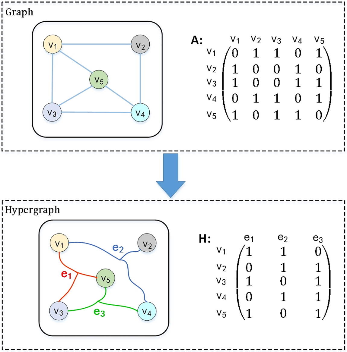
Figure 1: Comparison of graph and hypergraph structures

References [52,53] gave a specific definition of hypergraph. A hypergraph can be represented as GH=(VH,EH,WH,H) by the sets of nodes VH and hyperedges EH, where WH and H denote the hyperedge weight matrix and incidence matrix, respectively. Each hyperedge e∈EH is given a nonnegative weight w(e). The structure of the hypergraph can be described by a |VH|×|EH| dimensional incidence matrix H, in which h(v,e) denotes its specific element. In addition, a node v is located in a hyperedge e, h(v,e)=1, else h(v,e)=0. For each node v∈VH and hyperedge e∈EH, the degrees for the node d(v) and the degrees for the hyperedge d(e) are expressed as follows:

d(v)=∑e∈EHw(e)h(v,e)(1)

d(e)=∑v∈VHh(v,e)(2)

In addition, Dv is the diagonal matrix including the node degree d(v), and De is the diagonal matrix including the hyperedge degree d(e).

Hypergraph learning methods show a strong ability of higher-order spatial representation by means of information transfer between hypergraph structures [54]. GCN has a good learning ability in capturing non-Euclidian spatial features, but they over-rely on the adjacency matrix, thus ignoring the higher-order relations between nodes in graphs [55].

As the most prominent hypergraph learning model, HGCN is an important improvement of GCN in spatial modeling. The existing methods mainly adopt two modes: (1) It transforms hypergraph into simple graph, and then learns the spatial dependence through the GCN model. However, the transformation process is complicated, and the higher-order feature information is lost easily. (2) The node features of hypergraph are aggregated to form hypergraph features, and the new embeddings of each node are obtained from the hyperedge associated attributes. The feature transformation of graph structures is completed by the hyperedge convolution operation, so as to discover the potential hypergraph structural features [56]. Because the second mode learns the importance of nodes and hyperedges through the hyperedge feature transformation, it is suitable for the modeling of higher-order spatial features.

Take the second mode as an example. In the hypergraph neural network mentioned in reference [50], HGCN is expressed as:

X(l)=σ(Dv−1/2HWHDe−1HTDv−1/2X(l−1)Θ(l−1))(3)

where X(l) denotes the output values of the l-th layer, HT denotes the transpose of the incidence matrix H, σ is RELU activation function, and Θ is training parameters of the convolution layer.

4  Proposed Method

The change of traffic flow in a time window is dynamic and random, but also is of complex correlation, which brings some difficulties to the traffic spatiotemporal prediction. RLS will realize online estimation of system parameters, and have a great impact on model identification accuracy in the case of noises [57]. Meanwhile, EKF can be applied to nonlinear system prediction, but it is easy to be influenced by the accuracy of state estimation. In order to predict the traffic states of the road networks, as shown in Fig. 2, the method of HGC-NOM is proposed, which contains three factors: (1) the traffic flow of the forward timeslot; (2) the traffic flow of the historical simultaneous timeslot; and (3) the higher-order spatial aggregation value of the forward timeslot. Considering the effective integration of traffic data from multiple factors such as historical periods and higher-order spatial structures based on HGCN, the dynamic weights of different factors were identified by RLS, and traffic state vector values were updated online by the EKF algorithm, so as to improve the prediction accuracy in target segments.

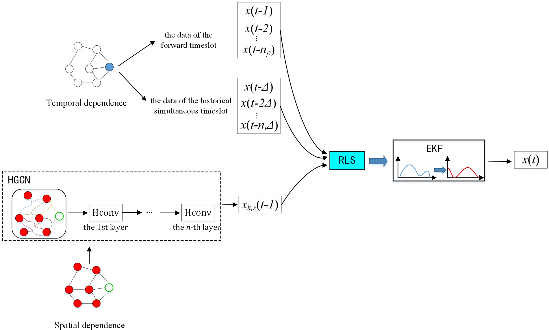
Figure 2: Overview of proposed HGC-NOM

4.1 HGCN Application

Due to the irregular structure of the traffic networks, traffic forecasting problem presents challenges that the spatial modeling of road network structures do not possess. At the same time, each node of road network structures has a different influencing degree on its adjacent areas. For example, the intersections near the business districts usually carry a larger traffic flow, which are bound to influence the predictive performance. HGCN will extract higher-order spatial features of road network structures according to the hyperedge correlation attributes, so as to accurately and comprehensively model complex spatial relationships.

According to the hypergraph GH=(VH,EH,WH,H) defined in Section 3, the hypergraph Laplacian matrix LH is constructed as follows:

LH=IN−Dv−1/2HWHDe−1HTDv−1/2(4)

where the diagonal matrix of the node degree Dv and the diagonal matrix of the hyperedge degree De are applied to the normalized incidence matrix H, respectively.

To reduce the computational complexity of feature space of incidence matrix H, Chebyshev polynomial is adopted to fit the convolution kernel gθ:

gθ(LH)∗x≈∑k=0KθkTk(L∼H)x(5)

where Tk and θk denote Chebyshev polynomials and coefficients, respectively. L∼H=2λmaxLH−IN, λmax denotes eigenvalue of maximum. In addition, Tk(L∼H)=2L∼HTk−1(L∼H)−Tk−2(L∼H), initial values T0(L∼H)=IN and T1(L∼H)=L∼H.

For the sake of simplicity, the eigenvalues of LH are scaled by setting K=1 and λmax=2, formula (5) is modified as follows:

gθ(LH)∗x≈θ0x+θ1(LH−IN)x≈θ0x−θ1Dv−1/2HWHDe−1HTDv−1/2(6)

To avoid overfitting, parameters θ0 and θ1 are fused into a unified parameter θ, which is defined as follows:

{θ0=12θDv−1/2HDe−1HTDv−1/2θ1=−12θ(7)

According to formulas (6), (7), the hypergraph convolution operation is derived as follows:

gθ(LH)∗x≈12θDv−1/2H(WH+IN)De−1HTDv−1/2≈θDv−1/2HWHDe−1HTDv−1/2(8)

Given the input matrix X∈Rn×c, where n and c represent the number of nodes and features, respectively. The output matrix Y can be expressed as:

Y=Dv−1/2HWHDe−1HTDv−1/2XΘ(9)

where Θ∈Rc×c denotes the training parameters of the convolution layer.

The convolution operation of the entire hypergraph convolution process is carried out according to the formulas (4)–(9), and the recursive calculation is combined with the nonlinear activation function σ. Finally, the convolution result of the l-th layer, that is the higher-order spatial aggregation value, is output, which is expressed as follows:

Y(l)=σ(Dv−1/2HWHDe−1HTDv−1/2Y(l−1)Θ(l−1))(10)

4.2 System Identification of RLS

The traffic flow in the historical simultaneous timeslots of the previous nt days, the traffic flow of the previous np timeslots during a day, and the target segment spatial value of the previous one timeslot xk,s(t−1) are selected. The spatial value xk,s(t−1) is calculated by the formulas (4)–(10). The following multiple regression equation for prediction is established:

x(t)=[a1a2⋯anp][x(t−1)x(t−2)⋮x(t−np)]+[b1b2⋯bnt][x(t−Δ)x(t−2Δ)⋮x(t−ntΔ)]+cxk,s(t−1)(11)

where x(t) is the predictive value of the road segment, x(t−1),⋯,x(t−np) are the traffic flow of the previous np timeslots during a day, Δ is the number of timeslots in a day (assuming the length of the timeslot and the number of timeslots remain constant), and x(t−Δ),⋯,x(t−ntΔ) are the traffic flow in the historical simultaneous timeslots of the previous nt days. a1…anp, b1…bnt and c are the influence weights of each system variable on the predictive value.

RLS is used to dynamically modify the existing results according to the new observed values, and the weighted estimator is adopted to estimate the parameters of different traffic states in real time. The state parameters are identified and updated according to formula (11). The transformed recursive equation is as follows:

x(t)=φkT(t)θ+ek(t)(12)

where φkT is the traffic flow of the road segment, θ is the identified parameter vector, and ek(t) is the error caused by observation noise. φkT and θ are recorded as vectors as follows:

φkT(t)=[x(t−1),…,x(t−np),x(t−Δ),…,x(t−ntΔ),xk,s(t−1)](13)

θ=[a1,…,anp,b1,…bnt,c]T(14)

Combining formulas (12)–(14), the system parameter identification gain and the error covariance matrix are updated. The least-squares equation is expressed as follows:

Kk(t)=Pk(t−1)φk(t)[φkT(t)Pk(t−1)θ^k(t−1)φk(t)+1]−1(15)

Pk(t)=[I−Kk(t)φk(t)T]Pk(t−1)(16)

where Kk(t) is the parameter identification gain for timeslot t, Pk is the error covariance matrix, and I is the identity matrix of the identification parameter.

According to formulas (12)–(16), the recursive formula for system parameter identification during timeslot t is expressed as follows:

θ^k(t)=θ^k(t−1)+Kk(t)[x(t−1)−φkT(t−1)θ^k(t−1)](17)

where θ^k is the least-squares estimate of the system parameters, and x(t−1)−φkT(t−1)θ^k(t−1) is the correction term of the identified parameter estimation for timeslot t−1.

4.3 Implementation of EKF

Kalman filter (KF) is a recursive method for optimal estimation of filter state variables. It is not only used for signal filtering estimation, but also for model parameter estimation, with static linearity and stability. KF mainly solves the filtering recursion problems of discrete linear data, and has been applied in the field of traffic prediction [58]. Since KF is a linear model, the performance of the model will be limited when predicting the nonlinear and random traffic states. EKF approximate linearizes the nonlinear state-space model, and adopts KF for traffic state estimation.

According to formula (11), the standard form of the state equation and the observation equation are expressed as follows:

{X(t)=f(X(t−1))+w(t−1)Y(t)=g(X(t))+m(t)(18)

where X(t) and Y(t) are state and observation vector values, respectively; w(t−1) is the system process noise; m(t) is the observation noise; and f(X(t−1)) and g(X(t)) are nonlinear mapping functions of the state equations and observation equations, respectively. X(t−1), f(X(t−1)), and g(X(t)) are expressed as follows:

X(t−1)=[x(t−1)⋯x(t−np)x(t−Δ)⋯x(t−ntΔ)xk,s(t−1)]T(19)

f(X(t−1))≈f(⌢X(t−1))+A(t−1)(X(t−1)−⌢X(t−1))(20)

g(X(t))≈g(⌢X(t))+B(t)(X(t)−⌢X(t))(21)

where ⌢X is the estimated value of X, and A and B are the system state matrix and the observation matrix, respectively.

According to formulas (18)–(21), A and B are derived as follows:

A(t−1)=∂f(X^(t−1))∂X(t−1)(22)

B(t)=∂g(X^(t))∂X(t)(23)

The two components of state vector X(t−1) in formula (19) are x(t−n) and xk,s(t−1). They are partial derivatives. A and B are converted to a Jacobian matrix:

{A(t−1)=[A1A2]B(t)=[10](24)

The corresponding parameters A1 and A2 in formula (24) are calculated as follows:

{A1=[a1,…,anp,b1,…bnt]TA2=c(25)

Since the specific values of parameters A1 and A2 corresponding to formula (25) are calculated by formula (17), then A(t−1) and B(t) are known values. Combining with the KF, the time update of formula (11) is expressed as follows:

X(t)−=f(X(t−1))(26)

P(t)−=A(t−1)P(t−1)+A(t−1)T+Q(27)

where X(t)− is the prior estimate of the state vector at timeslot t, P is the covariance of the state vector estimation error, and Q is the covariance matrix of the process noise.

According to formulas (18), (23), and (26), (27), the observation update of formula (11) is expressed as follows:

G(t)=P(t)−B(t)T(B(t)P(t)−B(t)T+R)−1(28)

P(t)+=(I−G(t)B(t))P(t)−(29)

X(t)+=X(t)−+G(t)(Y(t)−g(X(t)−))(30)

where G(t) is the Kalman gain at timeslot t, X(t)+ is the posterior estimate of the state vector at timeslot t, and R is the covariance matrix of the observation noise.

5  Experiments

5.1 Data Preparation

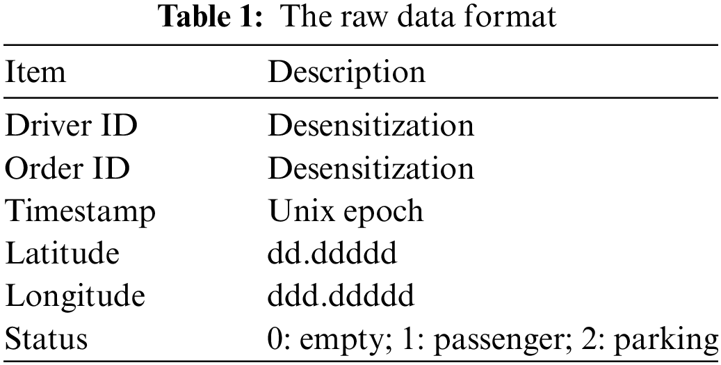
The dataset from the Chengdu branch of Didi Chuxing was adopted, the timespan is from October to November 2016. The geographic area is located at 30.66° N∼30.73° N, 104.02° E∼104.10° E, which is shown in Fig. 3. Three periods of traffic prediction in different road segments are adopted: the first and last weekdays, other weekdays, and weekends. All the dataset was downloaded from https://outreach.didichuxing.com. Each record includes: 1) driver ID; 2) order ID; 3) timestamp; 4) latitude; 5) longitude; and 6) vehicle status. The raw data format is shown in Table 1.

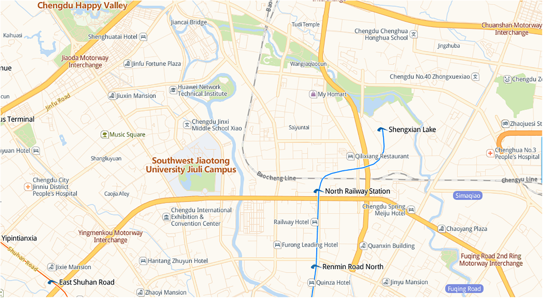
Figure 3: Geographical areas in Chengdu, China

The average speed was taken as the experimental data, and it was processed according to two-time steps (15 and 30 min). The travel speed is calculated as follows:

dtra=t int(v02+∑i=1k−1vi+vk2)(31)

vtra=dtratk−t0(32)

where dtra is the travel distance, tint is the fixed time interval, v(⋅) is the instantaneous speed, vtra is the travel speed, and t(⋅) is the GPS positioning time.

The instantaneous speed v is calculated as follows:

v=r∗arccos⁡{sin⁡(x1)∗sin⁡(x2)+cos⁡(x1)∗cos⁡(x2)∗cos⁡(y1−y2)}|T1−T2|(33)

where r is the earth radius, x1 and x2 are the latitudes of the adjacent positions, y1 and y2 are the longitudes of the adjacent positions, and T1 and T2 are the time stamps of the adjacent positions.

Thus, the formula for calculating the average speed is as follows:

v¯(t)=∑i=1nvtrai(t)/n(34)

where v¯(t) is the average speed during timeslot t, n is the number of travel speed samples, and vtrai(t) is the i-th travel speed at timeslot t.

To evaluate the performance of the proposed method, RMSE, MAE and MAPE were used as experimental evaluation metrics:

RMSE=1n∑in(v^(ti)−v¯(ti))2(35)

MAE=1n∑in|v^(ti)−v¯(ti)|(36)

MAPE=1n∑in|v^(ti)−v¯(ti)|v¯(ti)(37)

where v^(ti), v¯(ti) are the predicted value and estimated value at timeslot ti, respectively, and n is the timeslot number.

5.2 Comparative Results

The proposed method was compared with state-of-the-art methods for traffic prediction.

(1) RNN [59]: Recurrent neural network, a typical deep learning framework that uses neurons with self-feedback to recursively process various time-series data, including traffic prediction tasks.

(2) LSTM [60]: Long short-term memory network, a deep learning framework based on time loops, is suitable for predicting traffic information based on time series with long intervals.

(3) TGC-LSTM [61]: Based on the deep learning framework of GCN and LSTM, the correlation norm of graph convolution features is added to the loss function to learn the interaction between road segments, and predict the traffic states in traffic networks.

(4) DKFN [25]: The KF model based on deep neural network predicts the traffic states of the road network through the combination modeling of self-dependence and adjacent node dependence, and KF is used to optimize the predictive values.

(5) ST-GDN [62]: Spatial-temporal graph diffusion network, which learns not only a resolution-aware self-attention network to encode the multi-level temporal signals, but also the comprehensive high-order dependencies across different regions.

(6) HGC-NOM: The proposed method finds the high-order spatial characteristics of different segments through HGCN, uses RLS to dynamically weigh the spatiotemporal influencing factors of traffic flow, and adopts EKF to predict the traffic states of the road network.

(7) GC-NOM: This is a comparison for HGC-NOM, which combines the spatiotemporal factors and used EKF to predict the traffic states of the road network, but only find the spatial characteristics of different segments through GCN.

Table 2 shows the performance of the compared methods under different time steps. The conclusions are as follows:

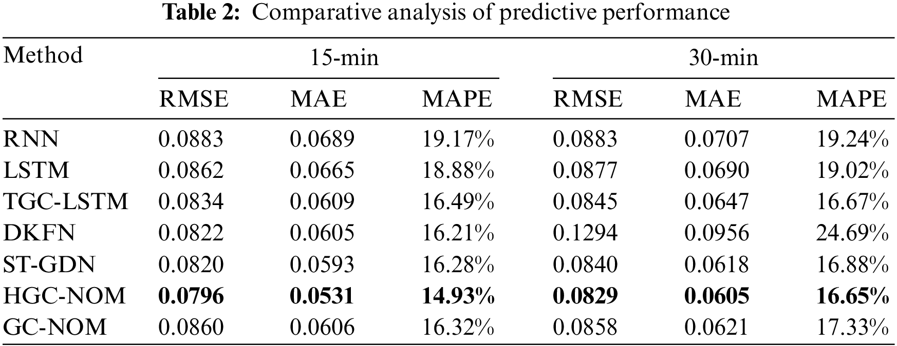
(1) From the perspective of the time scales, the three evaluation metrics of the compared methods all increase with the increase of the time step. A possible explanation for this may be that more traffic states belong to the same predictive unit with the expansion of the time step range, while the complexity and randomness of traffic environment bring some errors to the predictive evaluation.

(2) The proposed HGC-NOM method is superior to other compared methods in evaluation metrics. Especially at the 15-min time step, HGC-NOM has a more significant performance advantage. Compared with the second-best method, that is, ST-GDN, HGC-NOM achieves 3.0%, 11.7%, and 9.0% improvements in RMSE, MAE, and MAPE, respectively.

RNN and LSTM achieved good performance in traffic prediction based on temporal features. Since LSTM memorizes information through cell states, it has more advantages in predictive performance than RNN. By integrating GCN and LSTM, more accurate prediction results can be obtained. Compared with the single model LSTM, TGC-LSTM is more suitable for learning the spatiotemporal dependencies of the road network, and its performance is improved accordingly. DKFN utilizes the historical and spatial observation of adjacent nodes to dynamically adjust the weight coefficient of predictive model. In short-term (e.g., 15 min) traffic prediction, its performance is better than the previous three methods. Since KF is applied to linear systems, the randomness of traffic states increases with the increase of the time step, and the predictive performance significantly weakens under the 30-min time step. Compared to RNN, LSTM, TGC-LSTM, and DKFN, ST-GDN incorporates the global context enhanced region-wise explicit relevance into a graph diffusion paradigm to capture comprehensive high-order region dependencies. HGC-NOM achieved better performance than the above five methods. Meanwhile, the performance of HGC-NOM is also better than that of GC-NOM, which proves the efficiency of higher-order spatial features.

5.3 Feasibility

Combined with experimental data, the multiple regression equation in Section 4.2 contains three factors: (1) the average speed of the forward timeslot (AS-ft); (2) the average speed of the historical simultaneous timeslot (AS-hst); and (3) the higher-order spatial aggregation value of the forward timeslot (HSAV-ft). In order to demonstrate the influence of three factors on traffic prediction, according to the multiple regression equation, four influencing cases are selected. They respectively leave out the average speed of the forward timeslot (Miss-AS-ft), the average speed of the historical simultaneous timeslot (Miss-AS-hst), the higher-order spatial aggregation value of the forward timeslot (Miss-HSAV-ft), and without any missing factor (Normal-case).

In order to evaluate the predictive performance of different segments in road networks, we take the 15-min span as an example. The average speed during the rush hours (7 am–9 am and 5 pm–7 pm) in November, 2016 was selected. On this basis, three representative segments in a road network are taken (as shown in Table 3).

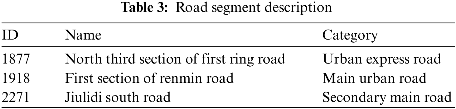
The RMSE of four influencing cases based on HGC-NOM are showed in Figs. 4–6, the acronyms “f_weekdays” and “o_weekdays” represent the first and last weekdays, and other weekdays,respectively.

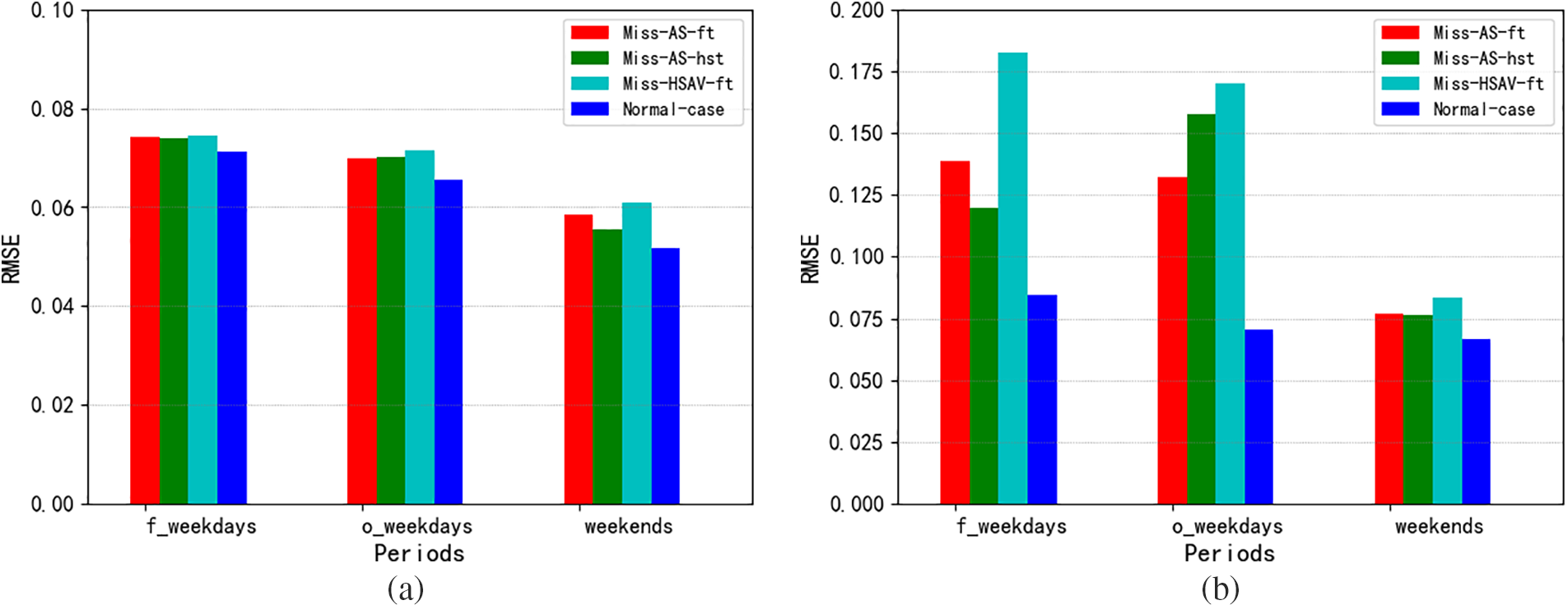
Figure 4: Performance of segment 1877 in morning rush hours (a) and evening rush hours (b)

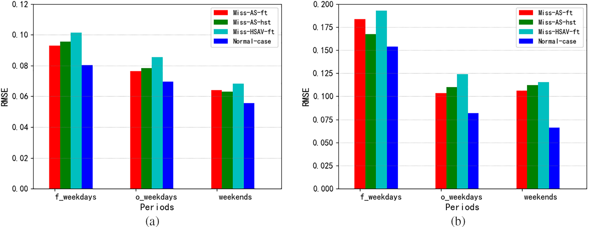
Figure 5: Performance of segment 1918 in morning rush hours (a) and evening rush hours (b)

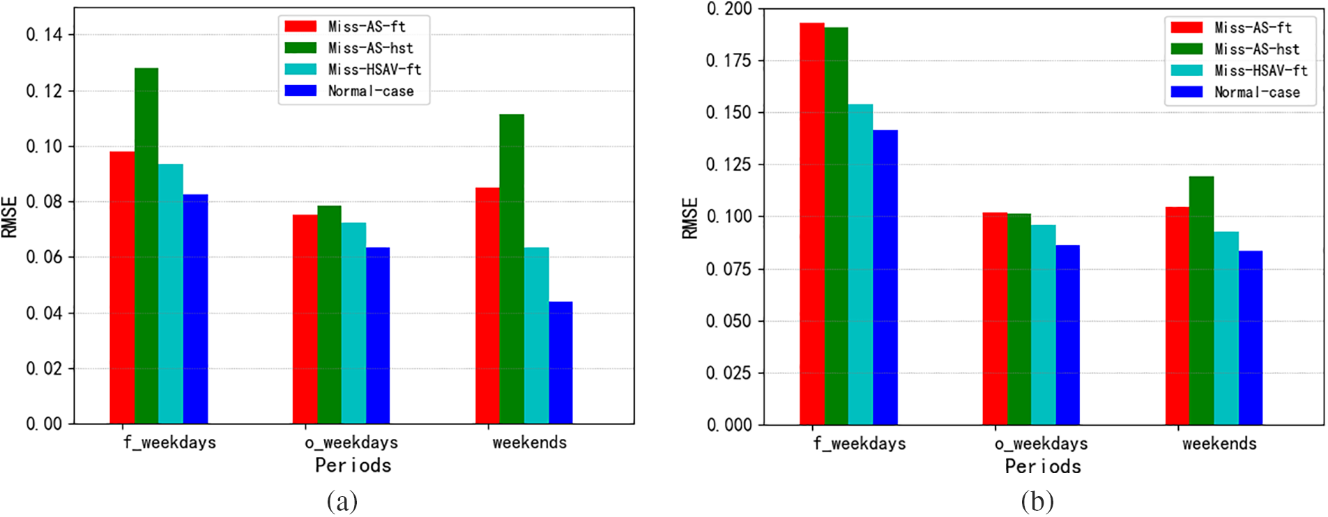
Figure 6: Performance of segment 2271 in morning rush hours (a) and evening rush hours (b)

From the perspective of road segment, the performance of segment 1877 is better than that of the other two roads at various periods. We take the Normal-case of evening rush hours as example, compared with segment 1918, segment 1877 achieves 82.4%, 15.9%, and 0.8% improvements in f_weekdays, o_weekdays, and weekends, respectively. In contrast to segment 2271, segment 1877 achieves 67.9%, 22.7%, and 25.7% improvements in f_weekdays, o_weekdays, and weekends, respectively. The possible reason is that segment 1877 is an urban express road. Compared with the main urban road and secondary main road, traffic interference of traffic signal and non-motor vehicle is relatively less, which may improve the prediction accuracy.

From the temporal perspective, the predictive performance of the three segments in morning rush hours is better than the performance in evening rush hours, especially there are more errors during the evening rush hour in the first and last weekdays. A possible reason is the heavy traffic flow of commuters on weekdays, whereas people traveled relatively less on weekends and traffic congestion weakened. At the same time, people traveled less on weekends or during normal hours, so its predictive performance is significantly better than the same time on weekdays.

From the perspective of the feature contribution of the four influencing cases, the larger the RMSE of the previous three cases, the greater the feature contribution to the proposed method. It can be seen that RMSE in the previous three cases are greater than those in the normal case, which verifies that the three influencing factors have different feature contributions to HGC-NOM. HSAV-ft contributes more to HGC-NOM in general, followed by AS-ft and AS-hst. At the same time, it is found that the influence of HSAV-ft weakens in the secondary main road, which may be that the correlated degree between the secondary main road and other types of road segments is relatively low.

6  Conclusions

In this paper, we propose an optimized method of traffic prediction (named HGC-NOM). It incorporates the higher-order spatial aggregation model HGCN and EKF algorithm to address two issues: 1) the limitation of capturing the spatiotemporal evolution characteristics of traffic states and 2) the lower-order connectivity of spatial structures. Combined with the high-order spatial features captured by HGCN, HGC-NOM dynamically adjusts the weight coefficients of the multiple regression equation in spatiotemporal dimensions through RLS, and utilizes EKF to reduce the nonlinear impact of the traffic environment. Based on the traffic data in Chengdu, China, an experiment validating the proposed method is carried out, and the result indicates that HGC-NOM achieves high accuracy. However, there still exist limitations while applying the proposed method to large-scale road networks, in future we will work toward improving the adaptation of the proposed method on higher-order spatial correlations.

Funding Statement: The authors received no specific funding for this study.

Conflicts of Interest: The authors declare that they have no conflicts of interest to report regarding the present study.

References

1. X. Yu, N. Ma, L. Zheng, L. Wang and K. Wang, “Developments and applications of artificial intelligence in music education,” Technologies, vol. 11, no. 2, pp. 42, 2023. https://doi.org/10.3390/technologies11020042 [Google Scholar] [CrossRef]

2. M. Zhang, W. Wang, G. Xia, L. Wang, K. Wang et al., “Self-powered electronic skin for remote human-machine synchronization,” ACS Applied Electronic Materials, vol. 5, no. 1, pp. 498–508, 2023. https://doi.org/10.1021/acsaelm.2c01476 [Google Scholar] [CrossRef]

3. M. Zhang, Y. Liu, D. Li, X. Cui, L. Wang et al., “Electrochemical impedance spectroscopy: A new chapter in the fast and accurate estimation of the state of health for Lithium-Ion batteries,” Energies, vol. 16,no. 4, pp. 1599, 2023. [Google Scholar]

4. J. Wang, Y. Zhang, L. Wang, Y. Hu, X. Piao et al., “Multitask hypergraph convolutional networks: A heterogeneous traffic prediction framework,” IEEE Transactions on Intelligent Transportation Systems, vol. 23,no. 10, pp. 18557–18567, 2022. [Google Scholar]

5. M. Zhang, D. Yang, J. Du, H. Sun, L. Li et al., “A review of SOH prediction of Li-Ion batteries based on data-driven algorithms,” Energies, vol. 16, no. 7, pp. 3167, 2023. [Google Scholar]

6. X. Zhou, W. Liang, K. Wang and L. T. Yang, “Deep correlation mining based on hierarchical hybrid networks for heterogeneous big data recommendations,” IEEE Transactions on Computational Social Systems, vol. 8, no. 1, pp. 171–178, 2021. [Google Scholar]

7. F. Wang, L. Wang, G. Li, Y. Wang, L. Chao et al., “Edge-cloud-enabled matrix factorization for diversified APIs recommendation in Mashup creation,” World Wide Web Journal, vol. 25, no. 5, pp. 1809–1829, 2022. [Google Scholar]

8. X. Zhou, W. Liang, K. Wang and S. Shimizu, “Multi-modality behavioral influence analysis for personalized recommendations in health social media environment,” IEEE Transactions on Computational Social Systems, vol. 6, no. 5, pp. 888–897, 2019. [Google Scholar]

9. L. Yang, Y. Zou, M. Xu, Y. Xu, D. Yu et al., “Distributed consensus for blockchains in Internet-of-Things networks,” Tsinghua Science and Technology, vol. 27, no. 5, pp. 817–831, 2022. [Google Scholar]

10. G. Shen, D. Zhu, J. Chen and X. Kong, “Motif discovery based traffic pattern mining in attributed road networks,” Knowledge-Based Systems, vol. 250, no. 1, pp. 109035, 2022. [Google Scholar]

11. D. Yu, Z. Zou, S. Chen, Y. Tao, B. Tian et al., “Decentralized parallel sgd with privacy preservation in vehicular networks,” IEEE Transactions on Vehicular Technology, vol. 70, no. 6, pp. 5211–5220, 2021. [Google Scholar]

12. L. Chen, L. Bei, Y. An, K. Zhang and P. Cui, “A hyperparameters automatic optimization method of time graph convolution network model for traffic prediction,” Wireless Networks, vol. 27, no. 7, pp. 4411–4419, 2021. [Google Scholar]

13. M. Murca and R. Hansman, “Identification, characterization, and prediction of traffic flow patterns in multi-airport systems,” IEEE Transactions on Intelligent Transportation Systems, vol. 20, no. 5, pp. 1683–1696, 2018. [Google Scholar]

14. J. Wang, R. Chen and Z. He, “Traffic speed prediction for urban transportation network: A path based deep learning approach,” Transportation Research Part C: Emerging Technologies, vol. 100, no. 2, pp. 372–385, 2019. [Google Scholar]

15. W. Li, J. Wang and R. Fan, “Short-term traffic state prediction from latent structures: Accuracy vs efficiency,” Transportation Research Part C: Emerging Technologies, vol. 111, no. 1, pp. 72–90, 2020. [Google Scholar]

16. Z. Cheng, W. Wang, J. Lu and X. Xing, “Classifying the traffic state of urban expressways: A machine-learning approach,” Transportation Research Part A: Policy and Practice, vol. 137, no. 4, pp. 411–428, 2020. [Google Scholar]

17. V. Arguedas, G. Pallotta and M. Vespe, “Maritime traffic networks: From historical positioning data to unsupervised maritime traffic monitoring,” IEEE Transactions on Intelligent Transportation Systems,vol. 19, no. 3, pp. 722–732, 2017. [Google Scholar]

18. W. Jiang and J. Luo, “Graph neural network for traffic forecasting: A survey,” Expert Systems with Applications, vol. 207, no. 7, pp. 117921, 2022. [Google Scholar]

19. Z. Zhang, P. Cui and W. Zhu, “Deep learning on graphs: A survey,” IEEE Transactions on Knowledge and Data Engineering, vol. 34, no. 1, pp. 249–270, 2022. [Google Scholar]

20. D. Zhu, G. Shen, J. Chen, W. Zhou and X. Kong, “A higher-order motif-based spatiotemporal graph imputation approach for transportation networks,” Wireless Communications & Mobile Computing, vol. 2022, no. 8, pp. 1702170, 2022. [Google Scholar]

21. J. Ye, J. Zhao, K. Ye and C. Xu, “How to build a graph-based deep learning architecture in traffic domain: A survey,” IEEE Transactions on Intelligent Transportation Systems, vol. 23, no. 5, pp. 3904–3924, 2022. [Google Scholar]

22. B. Yu, H. Yin and Z. Zhu, “Spatio-temporal graph convolutional networks: A deep learning framework for traffic forecasting,” in Proc. of IJCAI, Melbourne, Australia, pp. 3634–3640, 2017. [Google Scholar]

23. S. Guo, Y. Lin and N. Feng, “Attention based spatial-temporal graph convolutional networks for traffic flow forecasting,” in Proc. of AAAI, Honolulu, USA, pp. 922–929, 2019. [Google Scholar]

24. X. Ye, S. Fang, F. Sun, C. Zhang and S. Xiang, “Meta graph transformer: A novel framework for spatial-temporal traffic prediction,” Neurocomputing, vol. 491, no. 6, pp. 544–563, 2022. [Google Scholar]

25. F. Chen, Z. Chen, S. Biswas, L. Shuo and R. Naren, “Graph convolutional networks with Kalman filtering for traffic prediction,” in Proc. of 28th Int. Conf. on Advances in Geographic Information Systems, Seattle, USA, pp. 135–138, 2020. [Google Scholar]

26. M. Mansour, P. Davidson, O. Stepanov and R. Piché, “Towards semantic SLAM: 3D position and velocity estimation by fusing image semantic information with camera motion parameters for traffic scene analysis,” Remote Sensing, vol. 13, no. 3, pp. 388, 2021. [Google Scholar]

27. M. Saeedmanesh, A. Kouvelas and N. Geroliminis, “An extended Kalman filter approach for real-time state estimation in multi-region MFD urban networks,” Transportation Research Part C: Emerging Technologies, vol. 132, no. 2, pp. 103384, 2021. [Google Scholar]

28. X. Zhou, W. Liang, K. Yan, W. Li, K. Wang et al., “Edge enabled two-stage scheduling based on deep reinforcement learning for Internet of Everything,” IEEE Internet of Things Journal, vol. 10, no. 4, pp. 3295–3304, 2023. [Google Scholar]

29. X. Zhou, Y. Hu, J. Wu, W. Liang, J. Ma et al., “Distribution bias aware collaborative generative adversarial network for imbalanced deep learning in industrial IoT,” IEEE Transactions on Industrial Informatics,vol. 19, no. 1, pp. 570–580, 2023. [Google Scholar]

30. M. Xu, Z. Zou, Y. Cheng, Q. Hu, D. Yu et al., “SPDL: A blockchain-enabled secure and privacy-preserving decentralized learning system,” IEEE Transactions on Computers, vol. 72, no. 2, pp. 548–558, 2022. [Google Scholar]

31. H. Jing, Y. Zou, S. Zhang, J. Tang and Y. Wang, “Short-term speed prediction using remote microwave sensor data: Machine learning versus statistical model,” Mathematical Problems in Engineering, vol. 2016, no. 1965, pp. 9236156, 2016. [Google Scholar]

32. X. Kong, Z. Xu, G. Shen, J. Wang, Q. Yang et al., “Urban traffic congestion estimation and prediction based on floating car trajectory data,” Future Generation Computer Systems, vol. 61, no. 3, pp. 97–107, 2016. [Google Scholar]

33. Y. Liu, S. He, B. Ran and Y. Cheng, “A progressive extended Kalman filter method for freeway traffic state estimation integrating multisource data,” Wireless Communications & Mobile Computing, vol. 2018, pp. 6745726, 2018. [Google Scholar]

34. D. Zhu, G. Shen, D. Liu, J. Chen and Y. Zhang, “FCG-ASpredictor: An approach for the prediction of average speed of road segments with floating car GPS data,” Sensors, vol. 19, no. 22, pp. 4967, 2019. [Google Scholar] [PubMed]

35. L. Kong, G. Li, W. Rafique, S. Shen, Q. He et al., “Time-aware missing healthcare data prediction based on ARIMA model,” IEEE/ACM Transactions on Computational Biology and Bioinformatics, pp. 1–10, 2022. https://doi.org/10.1109/TCBB.2022.3205064 [Google Scholar] [CrossRef]

36. Q. Ye, W. Szeto and S. Wong, “Short-term traffic speed forecasting based on data recorded at irregular intervals,” IEEE Transactions on Intelligent Transportation Systems, vol. 13, no. 4, pp. 1727–1737, 2012. [Google Scholar]

37. J. Tang, F. Liu, Y. Zou, W. Zhang and Y. Wang, “An improved fuzzy neural network for traffic speed prediction considering periodic characteristic,” IEEE Transactions on Intelligent Transportation Systems, vol. 18, no. 9, pp. 2340–2350, 2017. [Google Scholar]

38. K. Zhang, L. Zheng, Z. Liu and N. Jia, “A deep learning based multitask model for network-wide traffic speed prediction,” Neurocomputing, vol. 396, pp. 438–450, 2020. [Google Scholar]

39. J. Zhang, Y. Zheng and D. Qi, “Deep spatio-temporal residual networks for citywide crowd flows prediction,” in Proc. of AAAI, San Francisco, USA, pp. 1655–1661, 2017. [Google Scholar]

40. Q. Wu, K. He, X. Chen, S. Yu and J. Zhang, “Deep transfer learning across cities for mobile traffic prediction,” IEEE Transactions on Networking, vol. 30, no. 3, pp. 1255–1267, 2021. [Google Scholar]

41. Y. Li, R. Yu, C. Shahabi and Y. Liu, “Diffusion convolutional recurrent neural network: Data-driven traffic forecasting,” in Proc. of ICLR, Vancouver, Canada, 2018. [Google Scholar]

42. F. Lu, Z. Zhang, L. Guo, J. Chen, Y. Zhu et al., “HFENet: A lightweight hand-crafted feature enhanced CNN for ceramic tile surface defect detection,” International Journal of Intelligent Systems, vol. 37, no. 12, pp. 10670–10693, 2022. [Google Scholar]

43. J. Chen, F. Qin, F. Lu, L. Guo, C. Li et al., “CSPP-IQA: A multi-scale spatial pyramid pooling based approach for medical image quality assessment,” Neural Computing and Applications, vol. 63, no. 11, pp. 1, 2022. https://doi.org/10.1007/s00521-022-07874-2 [Google Scholar] [CrossRef]

44. Z. Xie, Y. Huang, D. Yu, R. M. Parizi, Y. Zheng et al., “FedEE: A federated graph learning solution for extended enterprise collaboration,” IEEE Transactions on Industrial Informatics, 2022. https://doi.org/10.1109/TII.2022.3216238 [Google Scholar] [CrossRef]

45. Y. Zeng, J. Chen, N. Jin, X. Jin and Y. Du, “Air quality forecasting with hybrid LSTM and extended stationary wavelet transform,” Building and Environment, vol. 213, no. 9, pp. 108822, 2022. [Google Scholar]

46. C. Yu, X. Ma, J. Ren, H. Zhao and S. Yi, “Spatio-temporal graph transformer networks for pedestrian trajectory prediction,” in Proc. of European Conf. on Computer Vision, Glasgow, UK, pp. 507–523, 2020. [Google Scholar]

47. L. Zhao, Y. Song, C. Zhang, Y. Liu, P. Wang et al., “T-GCN: A temporal graph convolutional network for traffic prediction,” IEEE Transactions on Intelligent Transportation Systems, vol. 21, no. 9, pp. 3848–3858, 2020. [Google Scholar]

48. X. Ta, Z. Liu, X. Hu, L. Yu, L. Sun et al., “Adaptive spatio-temporal graph neural network for traffic forecasting,” Knowledge-Based Systems, vol. 242, pp. 108199, 2022. [Google Scholar]

49. L. Qi, W. Lin, X. Zhang, W. Dou, X. Xu et al., “A correlation graph based approach for personalized and compatible web APIs recommendation in mobile APP development,” IEEE Transactions on Knowledge and Data Engineering, vol. 9, pp. 1, 2022. https://doi.org/10.1109/TKDE.2022.3168611 [Google Scholar] [CrossRef]

50. Y. Feng, H. You, Z. Zhang, R. Ji and Y. Gao, “Hypergraph neural networks,” in Proc. of AAAI, Honolulu, USA, pp. 3558–3565, 2019. [Google Scholar]

51. L. Wu, D. Wang, K. Song, S. Feng, Y. Zhang et al., “Dual-view hypergraph neural networks for attributed graph learning,” Knowledge-Based Systems, vol. 227, no. 5, pp. 107185, 2021. [Google Scholar]

52. S. Fu, W. Liu, Y. Zhou and L. Nie, “HpLapGCN: Hypergraph p-Laplacian graph convolutional networks,” Neurocomputing, vol. 362, no. 12, pp. 166–174, 2019. [Google Scholar]

53. X. Ma, W. Liu, S. Li, D. Tao and Y. Zhou, “Hypergraph p-Laplacian regularization for remotely sensed image recognition,” Transactions on Geoscience and Remote Sensing, vol. 57, no. 3, pp. 1585–1595, 2019. [Google Scholar]

54. J. Wang, Y. Zhang, Y. Wei, Y. Hu, X. Piao et al., “Metro passenger flow prediction via dynamic hypergraph convolution networks,” IEEE Transactions on Intelligent Transportation Systems, vol. 22, no. 12, pp. 7891–7903, 2021. [Google Scholar]

55. Z. Ma, Z. Jiang and H. Zhang, “Hyperspectral image classification using feature fusion hypergraph convolution neural network,” Transactions on Geoscience and Remote Sensing, vol. 60, pp. 5517314, 2022. [Google Scholar]

56. S. Bai, F. Zhang and P. H. Torr, “Hypergraph convolution and hypergraph attention,” Pattern Recognition, vol. 110, no. 6, pp. 107637, 2021. [Google Scholar]

57. J. Kolansky and C. Sandu, “Enhanced polynomial chaos-based extended Kalman filter technique for parameter estimation,” Journal of Computational and Nonlinear Dynamics, vol. 13, no. 2, pp. 021012, 2018. [Google Scholar]

58. X. Xiong, K. Ozbay and L. Jin, “Dynamic origin-destination matrix prediction with line graph neural networks and Kalman filter,” Transportation Research Record, vol. 2674, no. 8, pp. 491–503, 2020. [Google Scholar]

59. Q. Liu, S. Wu, L. Wang and T. Tan, “Predicting the next location: A recurrent model with spatial and temporal contexts,” in Proc. of AAAI, Phoenix, USA, pp. 194–200, 2016. [Google Scholar]

60. R. Yu, Y. Li, C. Shahabi, U. Demiryurek and Y. Liu, “Deep learning: A generic approach for extreme condition traffic forecasting,” in Proc. of SDM, Houston, USA, pp. 777–785, 2017. [Google Scholar]

61. Z. Cui, K. Henrickson, R. Ke and Y. Wang, “Traffic graph convolutional recurrent neural network: A deep learning framework for network-scale traffic learning and forecasting,” IEEE Transactions on Intelligent Transportation Systems, vol. 21, no. 11, pp. 4883–4894, 2020. [Google Scholar]

62. X. Zhang, C. Huang, Y. Xu, L. Xia, P. Dai et al., “Traffic flow forecasting with spatial-temporal graph diffusion network,” arXiv:2110.04038, 2021. https://doi.org/10.48550/arXiv.2110.04038 [Google Scholar] [CrossRef]